A Model of Dual Fabry–Perot Etalon-Based External-Cavity Tunable Laser Using Finite-Difference Traveling-Wave Method

Abstract

A physical model of an external-cavity tunable laser (ECTL) utilizing the vernier effect of a dual Fabry–Perot (FP) etalon is presented and simulated using the finite-difference traveling wave (FDTW) method. In this paper, we provide a detailed explanation of the physical principle and construction process of the model, as well as the simulation results for the laser. The model is precisely established by studying the time-dependent changes in the carrier concentration and optical field of different wavelengths inside the laser before reaching a steady state. By determining multiple parameters in the tuning region and gain region, the proposed model can calculate and predict various laser parameters, such as output power and side-mode suppression ratio (SMSR). Moreover, the FDTW method displays the change process of various parameters, such as carrier concentration and spectrum, in the convergence of various positions in the laser with femtosecond time resolution. This capability is promising for in-depth research on the inner mechanism of lasers.

1. Introduction

Semiconductor lasers have attracted significant attention since their invention due to their small size, long lifetime, narrow linewidth, high-frequency modulation, and wide tunable range. In various application scenarios, laser performance requirements can differ significantly. For instance, in high-tech fields, such as high-resolution spectroscopy and broadband communication network systems, narrow-linewidth tunable semiconductor lasers are essential. External-cavity lasers provide a mature approach to fabricate narrow-linewidth tunable lasers. Using external-cavity technology, semiconductor lasers can produce stable single-longitudinal-mode output and can also be tuned in the range of tens to hundreds of nanometers [1]. Furthermore, several other properties of semiconductor lasers have been improved, including higher output power and greater SMSR [2]. Due to these desirable features, ECTLs have found wide usage in white-light interference, wavelength-division multiplexing (WDM) systems, optical coherence tomography, coherent optical communications, gas detection, atomic physics experiments, atomic clocks, and other fields.

Currently, there are several mature schemes for ECTLs, including the thermally tunable etalon type [3], MEMS-mechanical tuning type [4], acousto-optic (AO) filter type [5], and silicon-based double microring type [6]. Although MEMS-tuned external cavities and AO filters can achieve good lasing characteristics, their output power is limited. Moreover, MEMS-based ECTLs have mechanical parts and complex configurations, while those using AO filters have a large cavity length of 50 mm. Although ECTLs based on microring resonators have been extensively adopted due to their compact size and superior performance, FP etalons remain relevant for specialized applications where their unique advantages are indispensable. FP etalons exhibit a broader free spectral range (FSR) and reduced insertion loss compared to microring resonators, rendering them apt for scenarios where these attributes are of critical importance. For instance, FP etalons facilitate a wider tuning range and increased output power, which is attributed to their diminished insertion loss. Moreover, they exhibit reduced susceptibility to fabrication imperfections and environmental influences, resulting in enhanced stability and reliability under particular circumstances. In contrast, ECTLs prepared by an etalon can change the output frequency by modulating the FSR, combined with the wavelength position of the transmission peak of the etalon, to achieve the wavelength selection function [7]. This design can achieve high SMSR, low relative intensity noise (RIN), and narrow linewidth [8,9], thereby meeting the application requirements of WDM systems. The channel accuracy of the ECTL designed by K. Sato in the C-band with a channel spacing of 50 GHz is less than 0.6 GHz [10]. In 2018, Giovanni B. de Farias proposed an ECTL that meets the C-band Integrated Tunable Laser Assembly (ITLA) specification, and 16-quadrature amplitude modulation (QAM) transmission was verified [9]. These results demonstrate the excellent properties of ECTLs, but unfortunately, they lack further theoretical analysis. Moreover, existing theories [11] are limited to steady-state solutions, making it challenging to demonstrate the process of steady-state formation and track the change process of various physical quantities of a laser before reaching a steady state. Therefore, it is difficult to analyze the reasons for various results using these theories.

J. Leuthold proposed a fitted piecewise cubic curve to describe stimulated emission gain in relation to various measurable physical parameters in the gain region of a laser [12]. This model has been extensively used in numerous publications and textbooks [13,14,15]. In this study, we integrate the aforementioned gain model with the FDTW method [16,17]. The gain region is partitioned into independent input and output systems with distinct carrier concentration and optical field distribution, while the tuning region is treated as a power phase modulation system that is time invariant. By considering the time differential perspective, we simulate and explicate the steady state of the double-etalon external-cavity tunable laser. Lastly, we present the simulations of the steady-state laser spectra obtained from a series of measurable physical parameters. 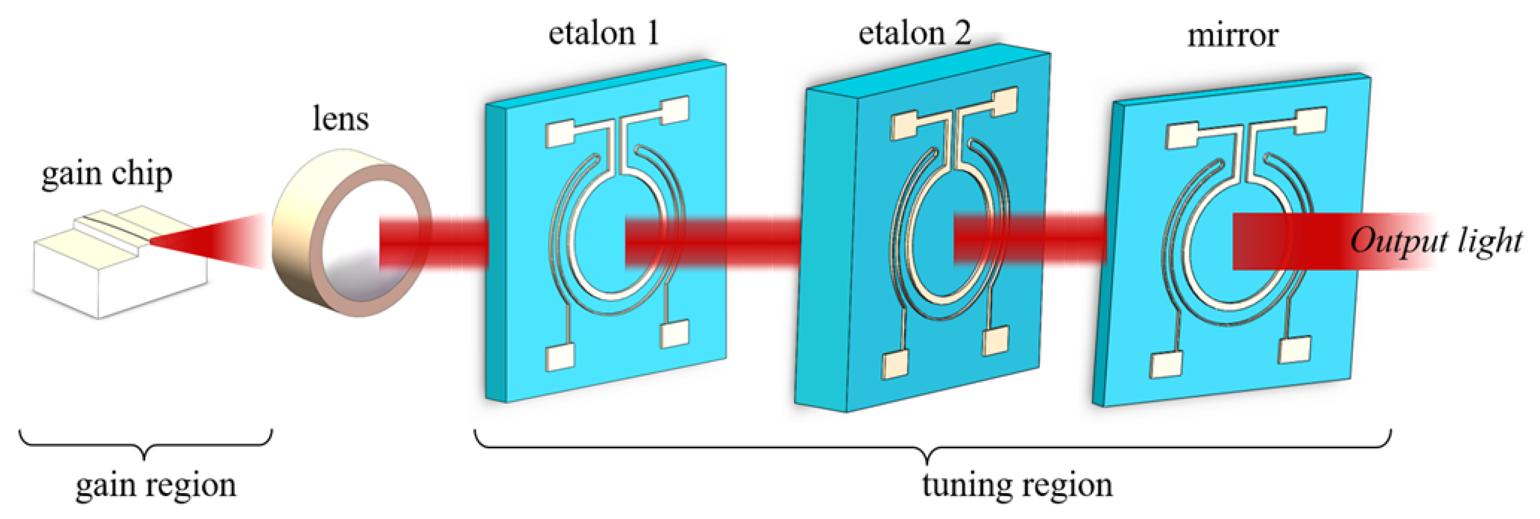Figure 1 displays the laser structure described in this article.

The structure of this paper is organized as follows: In Section 1, the transmission and reflection models for a tuning region that consists of two etalons are presented, along with a method for pre-selecting the FSR of the etalon. Section 3 describes the gain region model based on the work of J. Leuthold [12]. Section 4 introduces and discusses the simulation method used in this study. Section 5 presents the simulation results and a thorough discussion of the findings. Finally, in Section 6, the conclusions drawn from the research are presented.

2. Tuning Region

The tuning region comprises of two etalons and a reflector on the right, as depicted in Figure 1. The steady-state intensity transmission characteristics of the etalons can be explained using the current etalon filter power spectrum theory [18,19]. Since the etalons are a part of the laser resonator in our model, their impact on the optical path and phase of the cavity cannot be overlooked. The longitudinal-mode structure of the laser is determined by the longitudinal length of the resonator and the reflectivity of the reflector for the resonator formed by the etalons. 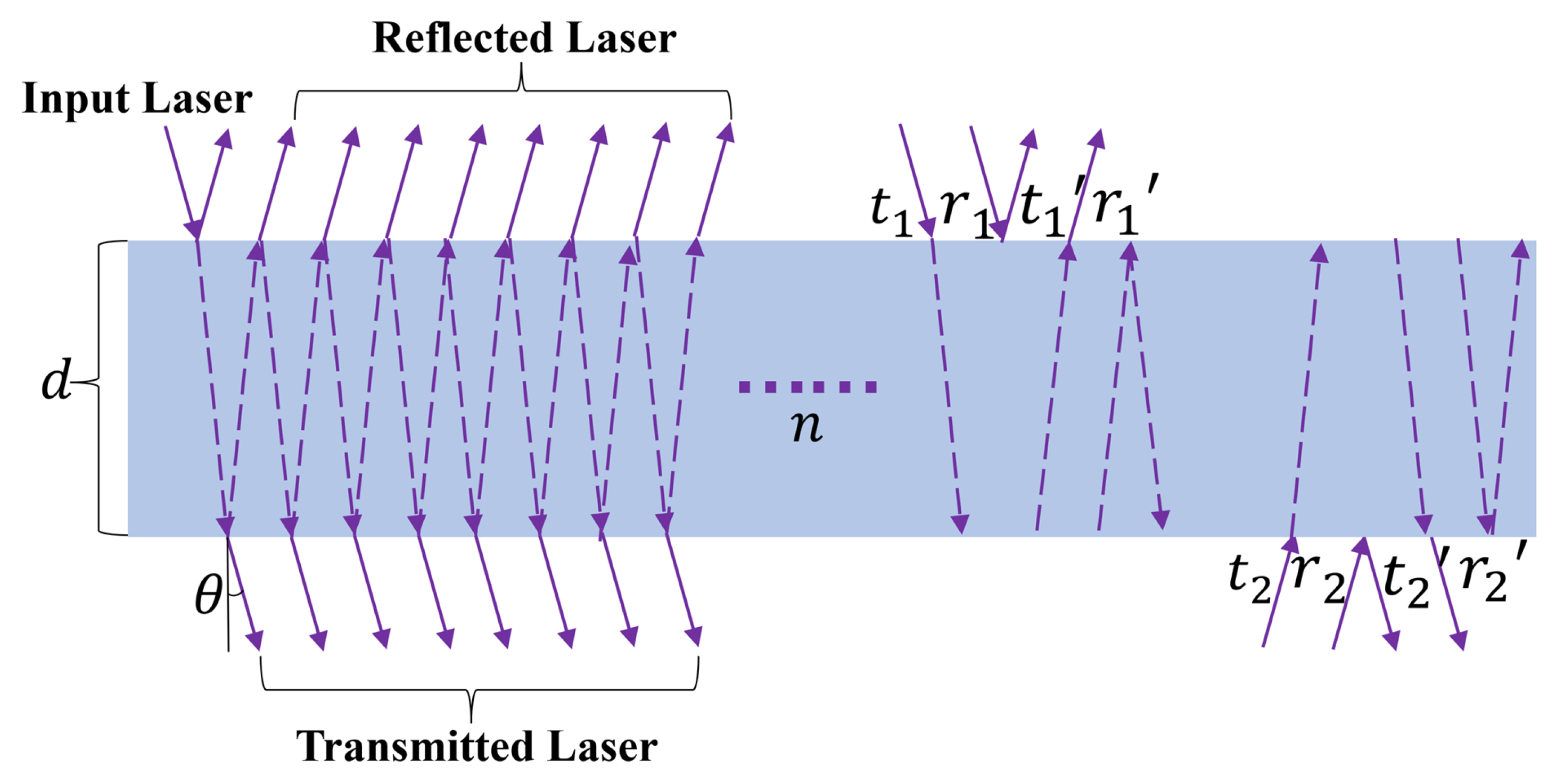Figure 2 shows the amplitude transmittance, amplitude reflectance, etalon internal refraction angle $\theta$, etalon refractive index $n$, and etalon thickness d of each surface. Considering the angle $\theta$ between the etalons and the optical axis, the continuous-wave field components accumulate discretely with the inclined angle, thus suppressing parasitic oscillations within the resonant cavity while inevitably introducing tilt loss. Consequently, as the filtering components within the cavity, we do not need to focus on the reflective behavior in the gap of the etalons; instead, we should concentrate on their transmission properties. By neglecting absorption, the following relationship is satisfied $\left(i=1,2\right)$:

$$\left\{\begin{array}{c}{r}_i=-r_i^{\prime }\hfill \\ r_i^2+t_i{t}_i^{\prime }=1\hfill \\ R_i=r_i^2\hfill \end{array}\right.$$

(1)

The intensity reflectivity of the two surfaces is denoted as $R_i$, and assuming $\lambda$ is the wavelength of the input laser, the phase difference $\delta$ caused by a round trip of the beam in the etalon satisfies the following relationship:

$$\delta =\frac{2nd\cos \theta }{\lambda }2\pi$$

(2)

Let $E_0$ be the input light-field amplitude, $E^{\prime }$ be the total transmitted light-field amplitude, $E$ be the total reflected light-field amplitude, and the amplitude transmittance be $t$, we have the following relationship:

$$t=\frac{E^{\prime }}{E_0}={\displaystyle \sum }_{N=1}^{+\infty }{t}_1{t}_2^{\prime }{r}_1^{\prime }{}^{N-1}{r}_2^{\prime }{}^{N-1}\exp \left[j\left(N-1\right)\delta \right]=\frac{\sqrt{\left(1-R_1\right)\left(1-R_2\right)}}{1-\sqrt{R_1{R}_2}\exp \left(j\delta \right)}$$

(3)

The corresponding total intensity transmission coefficients are as follows:

$$T=t{t}^{\ast }=\frac{\left(1-R_1\right)\left(1-R_2\right)}{{\left(1-\sqrt{R_1{R}_2}\right)}^2+4\sqrt{R_1{R}_2}{\sin }^2\left(\frac{\delta }{2}\right)}$$

(4)

When $R_1=R_2=R_0$, let the fineness parameter $F=4R_0/{\left(1-R_0\right)}^2$, and let the total phase difference $\Delta \phi ={tan}^{-1}{R}_0 sin \delta /\left(1-R_0 cos \delta \right)$, then

$$t=\frac{1-R_0}{1-R_0\exp \left(j\delta \right)}=\frac{1-R_0}{\sqrt{1+R_0^2-2\cos \delta }}\exp j\Delta \phi$$

(5)

$$T=\frac{1}{1+F{\sin }^2\left(\frac{\delta }{2}\right)}$$

(6)

The FSR and FWHM of the etalons are calculated as follows:

$$W_{FSR}=\left\{\begin{array}{cc}\frac{c}{2nd\cos \theta }\hfill & \hfill \hspace{1em} in Hz\\ \frac{1}{2nd\cos \theta }\hfill & \hfill \hspace{1em} in m^{-1}\\ \frac{{\lambda }^2}{2nd\cos \theta }\hfill & \hfill \hspace{1em} in m\end{array}\right.$$

(7)

$$W_{FWHM}=\frac{2W_{FSR}}{\pi \sqrt{F}}$$

(8)

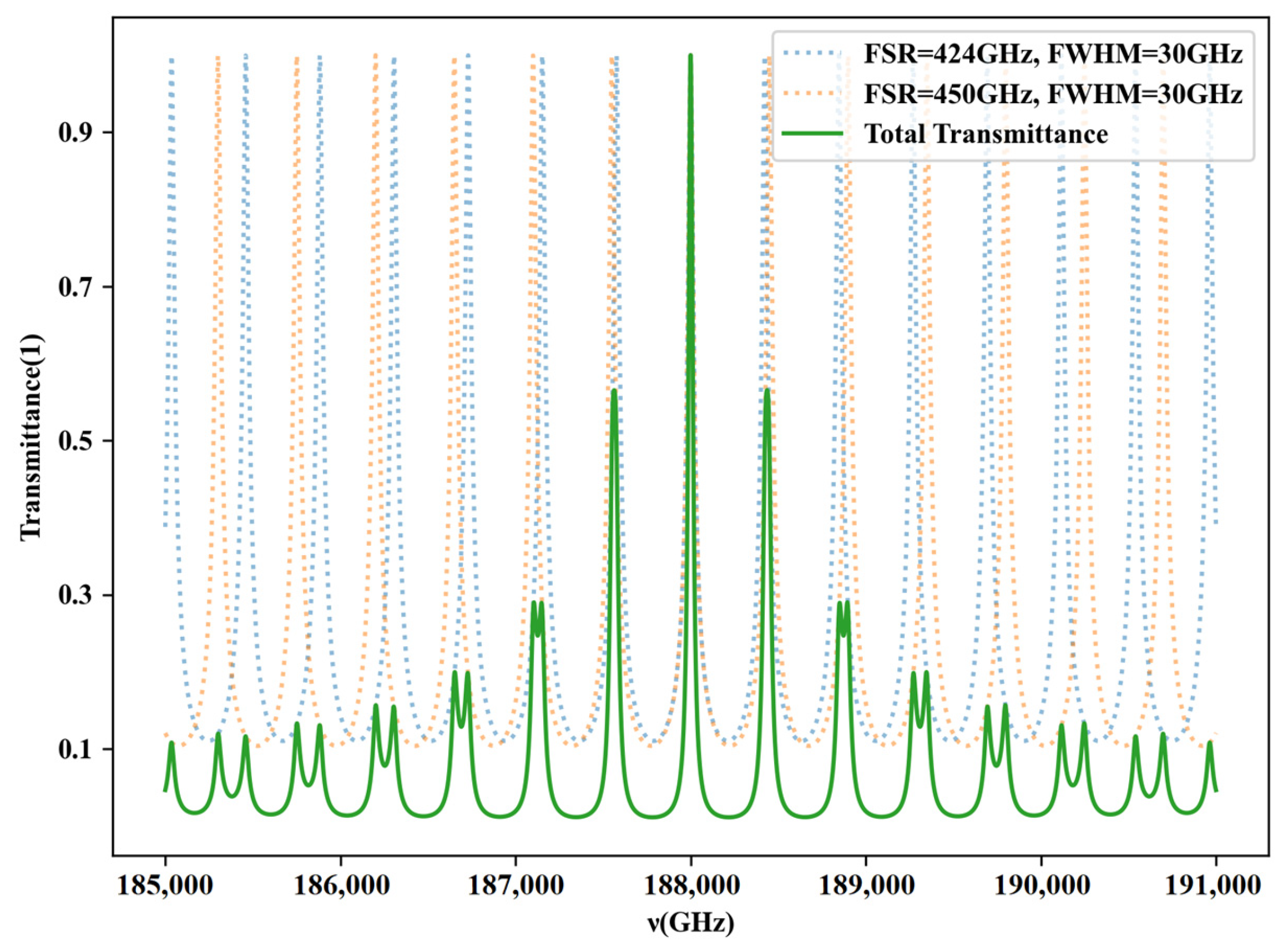
The transmission spectrum $T$ of the etalons can be completely determined by $W_{FSR}$ and $W_{FWHM}$, as shown in Figure 3.

A high side-mode suppression ratio (SMSR) is essential for external-cavity tunable semiconductor lasers as it influences spectral purity, system performance, signal stability, and the minimization of crosstalk and interference. This crucial parameter directly impacts the applicability and effectiveness of such lasers across various fields, including optical communication, sensing, metrology, and spectroscopy. The SMSR of a laser is determined by the tuning region and the gain region, each based on distinct mechanisms.

For the tuning region, given that the gain spectrum is sufficiently flat, the transmission spectrum’s SMSR within the tuning region will be directly reflected in the final spectrum. The gain chip will non-linearly exacerbate this process, ultimately resulting in the laser’s SMSR being significantly larger than the SMSR of the transmission spectrum in the tuning region [20].

Equations (5)–(8), in conjunction with Figure 3, demonstrate that the filtering properties of an etalon, such as the SMSR of the transmitted spectrum, are dependent on its $W_{FSR}$ and $W_{FWHM}$. In practical applications, it is often necessary to identify an appropriate combination of $W_{FSR}$ within a certain $W_{FWHM}$ while ensuring that the upper bound of the $W_{FSR}$ is not exceeded. This approach achieves the desired filtering performance when outputting specific wavelengths, such as 80 or 120 channels, within that band. The concept of finding such an FSR combination is as follows:

Expressing (4) with $W_{FSR}$ and $W_{FWHM}$, we have

$$T=\frac{1}{1+\frac{4W_{FSR}^2}{{\pi }^2{W}_{FWHM}^2}{\sin }^2\left(\frac{\nu \pi }{W_{FSR}}\right)}$$

(9)

which is simplified to

$$T\left(\Delta \nu \right)=\frac{1}{1+\frac{4\Delta {\nu }^2}{W_{FWHM}^2}}$$

(10)

The SMSR of the filter is ($\Delta \nu \in \left[0,\Delta W_{FSR}\right]$) as follows:

$$max\left[\frac{1}{1+\frac{4\Delta {\nu }^2}{W_{FWHM1}^2}}\times \frac{1}{1+\frac{4{\left(\Delta \nu -\Delta W_{FSR}\right)}^2}{W_{FWHM2}^2}}\right]$$

(11)

We traverse the possible FSR combinations and calculate the maximum value of their SMSR at the output of each band to select the most suitable FSR combination.

3. Gain Region

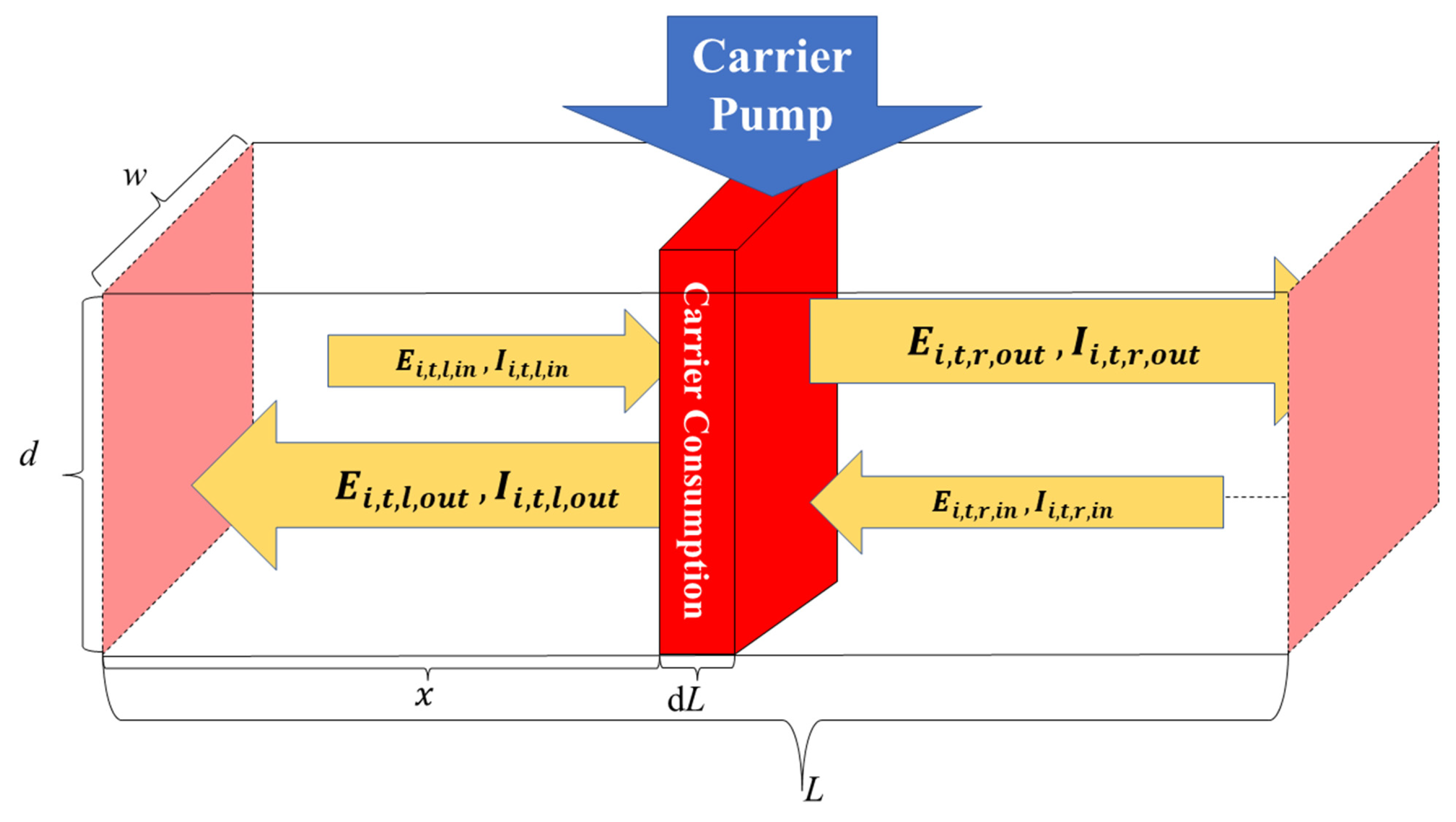
The gain region consists of the gain medium, which is electrically pumped to realize carrier concentration inversion, and the results in the stimulated emission optical gain for the incident light while also spontaneously emitting broad-spectrum fluorescence. The processes of spontaneous and stimulated emissions, as well as non-radiative transitions, together consume inversion carriers, and a constant current generates inversion carriers at a constant rate. The following analysis focuses on the changes in various related parameters as light passes through a thin layer in the gain region, as illustrated in Figure 4.

During the time interval $\mathrm{d} t=\mathrm{d} x\times n_g/c$, when photons travel from the left surface to the right surface of the thin layer, the reverse carrier concentration in the thin layer is pumped by the injection current in the gain region. The depletion of the inverse carrier concentration in the thin layer is caused by nonradiative recombination, spontaneous emission, Auger recombination, and stimulated emission. The changes in electron concentration and photon concentration during this time interval are given by [16]:

$$\frac{dN}{dt}=\frac{\eta I_{inject}}{qwdL}-AN-B{N}^2-C{N}^3-{{\displaystyle \int }}_{-\infty }^{+\infty }g\left(\lambda ,N\right)N_P\left(\lambda \right)\frac{c}{n_g}d\lambda$$

(12)

$$\frac{d N_P\left(\lambda \right)}{d t}=\Gamma \frac{c}{n_g}g\left(\lambda ,N\right)N_P\left(\lambda \right)+\Gamma \beta B\left(\lambda \right)N^2$$

(13)

The relationship between photon concentration and electric-field strength density is as follows:

$$N_P\left(\lambda \right)=\frac{2{\epsilon }_0{n}_{eff}{n}_g}{h\nu }{\left|E\left(\lambda \right)\right|}^2$$

(14)

For its rate of change in amplitude, we have the following:

$$d\left|E_{spon}\left(\lambda \right)\right|=\sqrt{\frac{h\nu }{4{\epsilon }_0{n}_{eff}{n}_g}}\frac{\Gamma \beta B\left(\lambda \right)N^2}{\sqrt{N_P\left(\lambda \right)}}dt$$

(15)

$$d\left|E_{stim}\left(\lambda \right)\right|=\sqrt{\frac{h\nu }{4{\epsilon }_0{n}_{eff}{n}_g}}\Gamma \frac{c}{n_g}g\left(\lambda ,N\right)\sqrt{N_P\left(\lambda \right)}$$

(16)

After $dx$, the phase change is as follows:

$$d \phi =\frac{2\pi n_{g}d x}{\lambda }$$

(17)

Thus, for the total light-field amplitude change, we have the following:

$$E_{out}\left(\lambda \right)=e^{i\left({\phi }_0+d \phi \right)}\left(\left|E_{in}\left(\lambda \right)\right|+d\left|E_{stim}\left(\lambda \right)\right|\right)+e^{i{\phi }_r}d\left|E_{spon}\left(\lambda \right)\right|$$

(18)

where ${\phi }_0$ is the phase of $E_{in}\left(\lambda \right)$ and ${\phi }_r$ is a uniformly distributed random phase.

Next, we discuss the gain parameter $g\left(\lambda ,N\right)$. We use a polynomial model for the material gain to describe $g\left(\lambda ,N\right)$ at a specific carrier concentration [12]:

$$g\left(\lambda ,N\right)=\left\{\begin{array}{cc}{c}_N{\left[\lambda -{\lambda }_z\left(N\right)\right]}^2+d_N{\left[\lambda -{\lambda }_z\left(N\right)\right]}^3\hfill & ,\lambda <{\lambda }_z\left(N\right)\\ 0\hfill & ,\lambda \ge {\lambda }_z\left(N\right)\end{array}\right.$$

(19)

where

$$c_N=3\frac{g_p\left(N\right)}{{\left[{\lambda }_z\left(N\right)-{\lambda }_p\left(N\right)\right]}^2}$$

(20)

$$d_N=2\frac{g_p\left(N\right)}{{\left[{\lambda }_z\left(N\right)-{\lambda }_p\left(N\right)\right]}^3}$$

(21)

$$g_p\left(N\right)=a_0\left(N-N_0\right)+\overline{a}{a}_0{N}_0 \exp -\frac{N}{N_0}$$

(22)

$${\lambda }_p\left(N\right)={\lambda }_0-[b_0\left(N-N_0\right)+b_1{\left(N-N_0\right)}^2]$$

(23)

$${\lambda }_z\left(N\right)={\lambda }_z{}_0-z_0\left(N-N_0\right)$$

(24)

Up to this point, we have determined two important parameters of the gain region: the gain coefficient $g\left(\lambda \right)$ and the coefficient $B$ for spontaneous radiative recombination.

To use the above model for laser simulations, several parameters of the tuning region and the gain region must be determined before the FDTW method can be applied [16,17]. See

Table 1. Parameters appearing in the model.

Symbol	Value	Parameter
$q$	$1.602\times {10}^{-19} \mathrm{C}$	Electron charge
$c$	$2.998\times {10}^8 \mathrm{m}/\mathrm{s}$	The speed of light in vacuum
$h$	$6.625\times {10}^{-34} \mathrm{J}·\mathrm{s}$	Planck’s constant
${\epsilon }_0$	$8.854\times {10}^{-12} \mathrm{F}/\mathrm{m}$	Vacuum dielectric constant
$\Delta \lambda$	$1 \mathrm{nm}$	Wavelength interval of our work
$w$	$2 \mathsf{\mu }\mathrm{m}$	The width of the gain region
$d$	$0.2 \mathsf{\mu }\mathrm{m}$	The thickness of the gain region
$L$	$1 \mathrm{mm}$	The length of the gain region
$\Delta L$	$1 \mathsf{\mu }\mathrm{m}$	The length of the gain slice
$A$	$1.25\times {10}^8$	Unimolecular non-radiative recombination coefficient
$B$	$0.8\times {10}^{-16}{ \mathrm{m}}^3/\mathrm{s}$	Bimolecular spontaneous radiative recombination coefficient
$C$	$0.9\times {10}^{-42}{ \mathrm{m}}^6/\mathrm{s}$	Auger recombination coefficient
$\eta$	$0.7$	Current injection efficiency
$W_{FSR1}$	$424 \mathrm{GHz}$	The FSR of the first etalon at room temperature
$W_{FSR2}$	$450 \mathrm{GHz}$	The FSR of the second etalon at room temperature
$W_{FWHM1}$	$10 \mathrm{GHz}$	The FWHM of the first etalon at room temperature
$W_{FWHM2}$	$10 \mathrm{GHz}$	The FWHM of the second etalon at room temperature
$N_0$	$6.5\times {10}^{23}{ \mathrm{m}}^{-3}$	Transparency carrier density
$a_0$	$3.13\times {10}^{20}{ \mathrm{m}}^2$	Differential gain factor
${\lambda }_0$	$1.575\times {10}^6 \mathsf{\mu }\mathrm{m}$	Band-edge wavelength
$b_0$	$3.17\times {10}^{32}{ \mathrm{m}}^3\mathsf{\mu }\mathrm{m}$	Peak wavelength shift coefficient
${\lambda }_{z_0}$	$1.625\times {10}^6 \mathsf{\mu }\mathrm{m}$	Begin-to-zero gain region
$z_0$	$-2.5\times {10}^{33}{ \mathrm{m}}^3\mathsf{\mu }\mathrm{m}$	Zero-gain wavelength shift coefficient

for the details of the parameters.

4. Simulation

In this simulation, all the light-field behavior of the laser at a certain position and time is determined by the left-direction and right-direction complex-amplitude vectors at that position, which are composed of n + 1 complex numbers (where $n=({\lambda }_{end}-{\lambda }_{start})/\Delta \lambda$), with each complex number representing the complex amplitude of the light field at a specific frequency.

In order to simulate the gain region, we partition it into a finite number of slices at equal intervals along the propagation direction of the light field, where the step size is denoted by $\Delta x$, as illustrated in Figure 4. It is assumed that the injection current in the gain region remains constant until the steady state is reached. During the tiny time interval $\Delta t=n_g\Delta x/c$, when the envelope of the optical field amplitude passes through the slice at a group velocity of $c/n_g$, the carrier concentration remains constant. 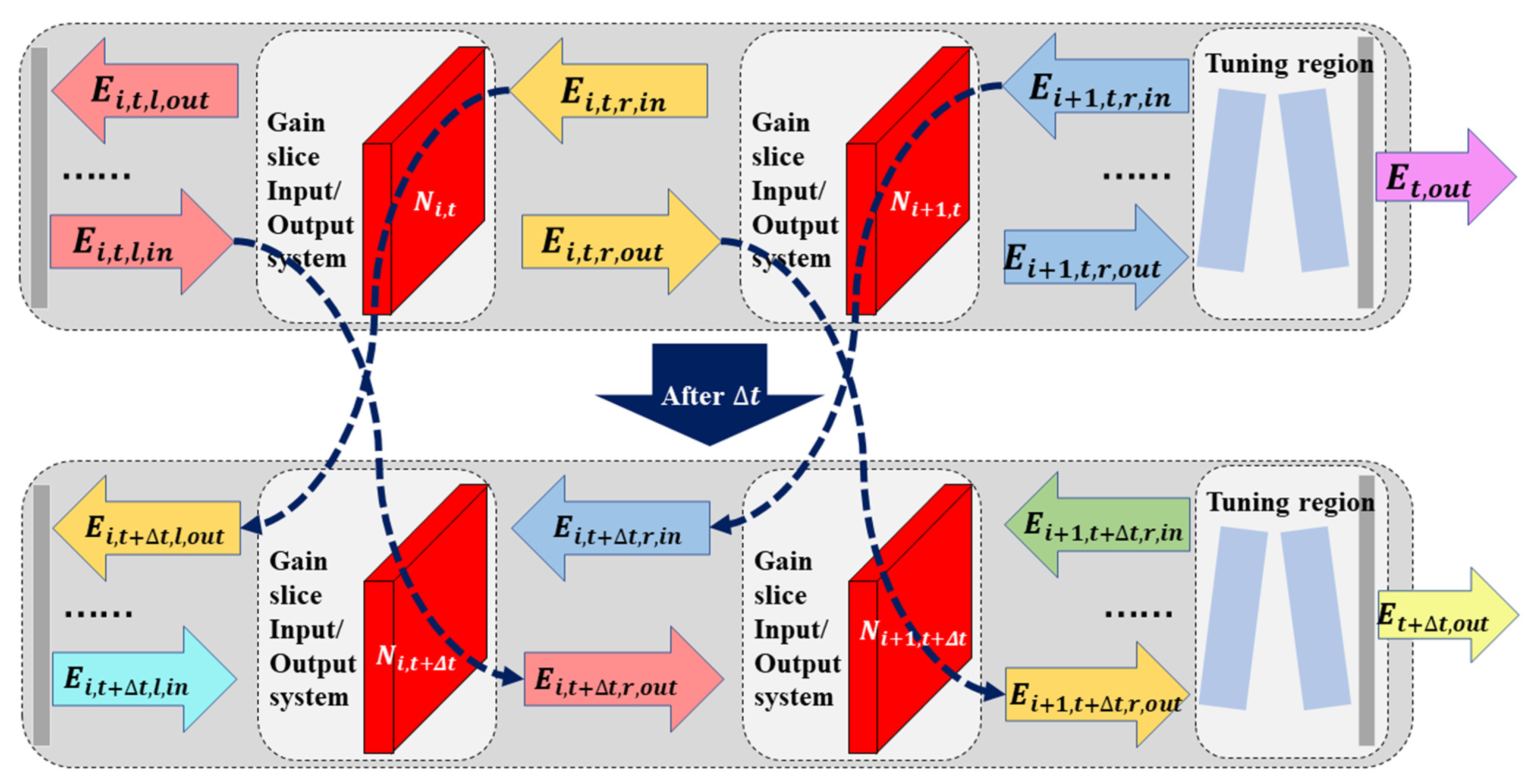Any carrier concentration that is consumed or generated during this process will act on the slice after $\Delta t$, thereby forming a gain sheet input–output system.

The gain region comprises $n$ $\left(n=L/\Delta L\right)$ gain slice input and output systems connected in series. At a given time $\left(t=m\Delta t, \mathrm{where} m=0,1,2,\dots \right)$, the outputs of adjacent gain slice systems are connected to the inputs of the next system at the start of the next time interval $\Delta t$. Specifically, for the leftmost gain sheet system, the left input light field is always the product of the left output light field and $\sqrt{R_{left}}$, while for the rightmost gain sheet system, the input light field on the right is always the product of the output light field on the right and $r_{tuning}\left(\lambda \right)$. The propagation time of the light field in the tuning region is neglected, as this region is treated as passive and its physical quantities do not vary during our analysis. Moreover, the process of establishing the steady state inside the tuning region is not the focus of our study. The neglect of the propagation of the tuning region does not affect the overall steady state of the laser. The gain region, formed by the gain slices in series, is depicted in Figure 5.

At the outset, the n gain slices in the gain region exhibit no gain, and the reverse carrier concentration arises from the injection current generation in the gain region and the consumption of non-radiative recombination, spontaneous emission, and Auger recombination. This carrier concentration is determined by the steady state, which takes the following form:

$$\frac{\eta I_{inject}}{qwdL}-\left(A{N}_{0,i}+B{N}_{0,i}{}^2+C{N}_{0,i}{}^3\right)=0$$

(25)

The inversion carrier concentration $N_{0,i}$ of the initial state can be determined, with the carrier concentration being the same for each sheet. The next step is to examine the input and output states of each gain slice in the initial state. As no gain exists in the initial state, the left and right outputs of each slice correspond to their spontaneous emission, with the following values:

$$E_{initial}\left(\lambda \right)=\sqrt{\frac{h\nu wd\Delta L{N}_{0,i}}{2{\epsilon }_0{n}_{eff}{n}_g}}{e}^{i{\phi }_r}$$

(26)

In the initial state, the electric-field strength within the gain region is denoted by $E_{initial}\left(\lambda \right)$ at each corresponding wavelength.

Next, we discuss the boundary conditions for iterative processes. Specifically, for the leftmost slice, the input on the left is always equal to the product of the output on the left and the reflectivity of the left mirror amplitude. This can be expressed as follows:

$$E_{1,t+\Delta t,l,in}\left(\lambda \right)=\sqrt{R_{left}}\times E_{1,t,l,out}\left(\lambda \right)$$

(27)

The initial numeral denotes the slice number from left to right. In the aforementioned equation, we are specifically referring to the leftmost slice, hence denoted by ‘1’. The second numeral corresponds to time. The third symbol signifies the position of the light field, where ‘l’ denotes the left surface of the sheet, and ‘r’ represents the right surface of the sheet. The final symbol signifies either incoming or outgoing light of the slice, where ‘in’ refers to incoming light and ‘out’ refers to outgoing light.

Regarding the rightmost slice, it can be observed that its input consistently equals the multiplication of the right output and the amplitude reflectance of the tuning region:

$$E_{1,t+\Delta t,r,in}\left(\lambda \right)=r_t\left(\lambda \right)\times E_{1,t,r,out}\left(\lambda \right)$$

(28)

The power of the light emitted at any time is calculated as follows:

$$P\left(\lambda \right)=\frac{2{\left|E_{n,t,r,out}\left(\lambda \right)\right|}^2{\epsilon }_0}{\Delta t}$$

(29)

Next, we examine the changes in the optical field and the carrier concentration for each slice per unit time $\Delta t$ during the iteration.

Within each slice, as each time interval $\Delta t$ elapses, we analyze the correlation between the output light field of all slices and the input light field in the corresponding direction using Equation (18), which can be expressed as follows:

$$E_{n,t+\Delta t,l,out}\left(\lambda \right)=f_E\left(E_{n,t,r,in}\left(\lambda \right),N_{i,t}\right)$$

(30)

$$E_{n,t+\Delta t,r,out}\left(\lambda \right)=f_E\left(E_{n,t,l,in}\left(\lambda \right),N_{i,t}\right)$$

(31)

Simultaneously, the evolution of the carrier concentration is governed by Equation (12), which can be formulated as follows:

$$N_{i,t+\Delta t}=f_N\left(N_{i,t},E_{n,t,r,in}\left(\lambda \right),E_{n,t,l,in}\left(\lambda \right)\right)$$

(32)

For slices located between the leftmost and rightmost slices, during each time interval $\Delta t$, the input light field of a given slice is determined by the output light field of its adjacent neighbor at the preceding moment. This relationship can be expressed as follows:

$$E_{n,t+\Delta t,l,in}\left(\lambda \right)=E_{n-1,t,r,out}\left(\lambda \right)$$

(33)

$$E_{n,t+\Delta t,r,in}\left(\lambda \right)=E_{n+1,t,l,out}\left(\lambda \right)$$

(34)

Once the essential parameters, boundary conditions, and initial conditions have been established, the iterative process can commence. The iteration continues until the results converge or until a reasonable amount of time has passed, at which point all relevant physical parameters will have been determined.

5. Results

Compared to the simulation results obtained by other models, our proposed model provides a comprehensive visualization of the dynamic changes in various physical quantities over time, rather than just the final converged results. Additionally, our model simplifies the time-domain behavior of the two etalons in the tuning region, resulting in a faster convergence speed than the actual situation while preserving the spectral and energy changes without affecting the laser’s lasing spectrum. Using this model, we can explain and predict various physical phenomena and laws observed in the longitudinal-mode behavior of a laser, as demonstrated in Figure 6 and Figure 7, from a more microscopic perspective.

In the absence of any specific instructions regarding parameter settings in this paper, the following default values are adopted: injection current $I=0.1 \mathrm{A}$, reflectivity of the mirror on the right side of the tuning area $R=0.5$, and output wavelength $\lambda =1590 \mathrm{nm}$. Please refer to Table 1 for the remaining parameter values.

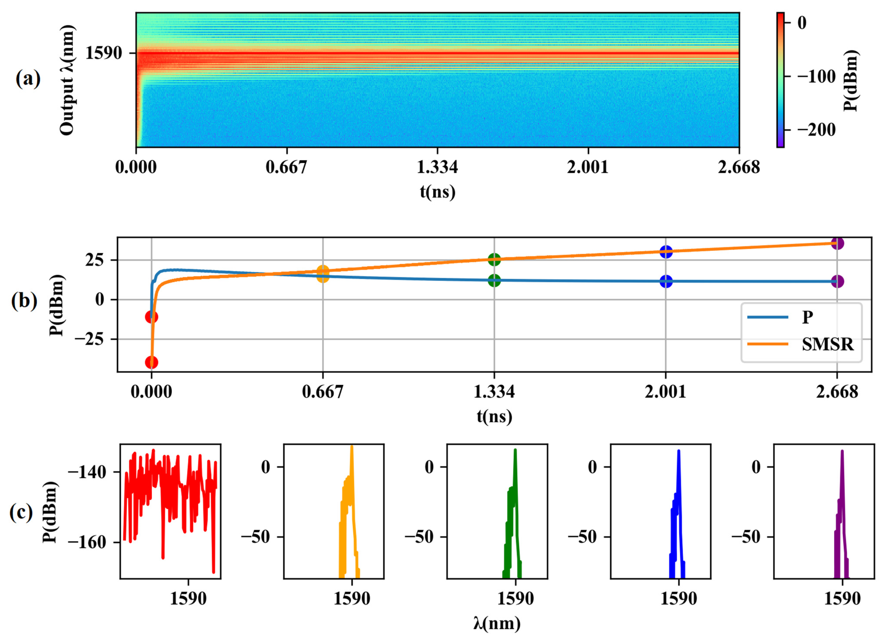
In Figure 6, the wavelengths studied were selected based on the maximum points of the transmission spectrum in the tuning region, thus allowing us to examine various physical quantities with minimal computational effort. As shown in Figure 6a, the side modes briefly disappear before the main mode narrows. Figure 6b indicates that the power converges more quickly than the SMSR due to the faster convergence of the average carrier concentration, while the convergence process of the carrier concentration distribution is slower, leading to the slower convergence of the secondary mode. Figure 6c shows that the selection process of the main mode is rapid, but the spectral line shaping takes longer.

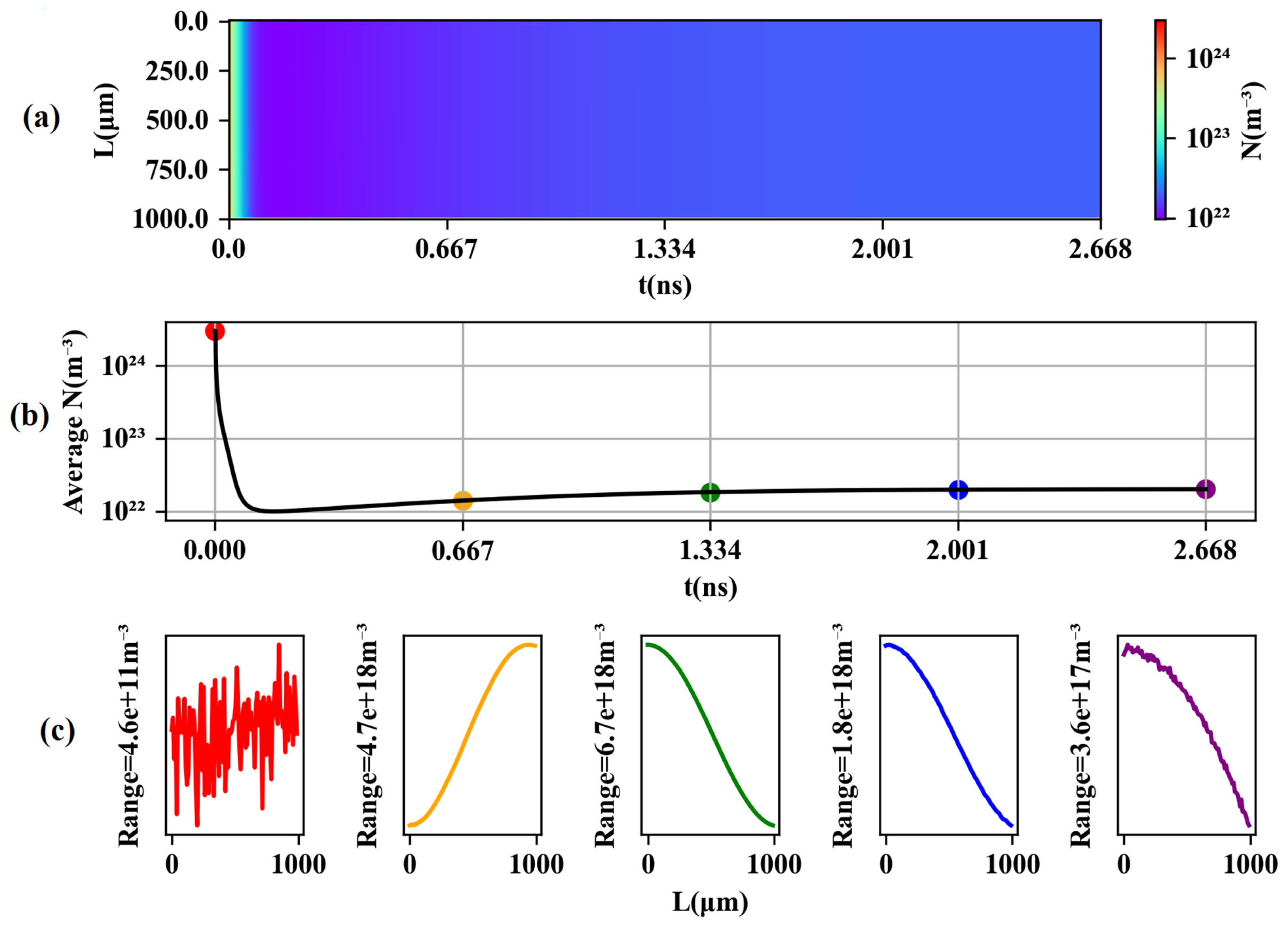
The reverse carrier concentration exhibits an opposite trend to the output power. In Figure 7, we see a rapid drop in the carrier concentration, followed by a slow rise and eventual convergence to a steady state. This is due to the consumption of inversion carriers during lasing and a gain clamping effect. The gradient of the spatial distribution of carriers is relatively small compared to the change in carrier concentration over time, and carrier concentration near the output side is slightly lower due to the stronger optical field and greater carrier consumption.

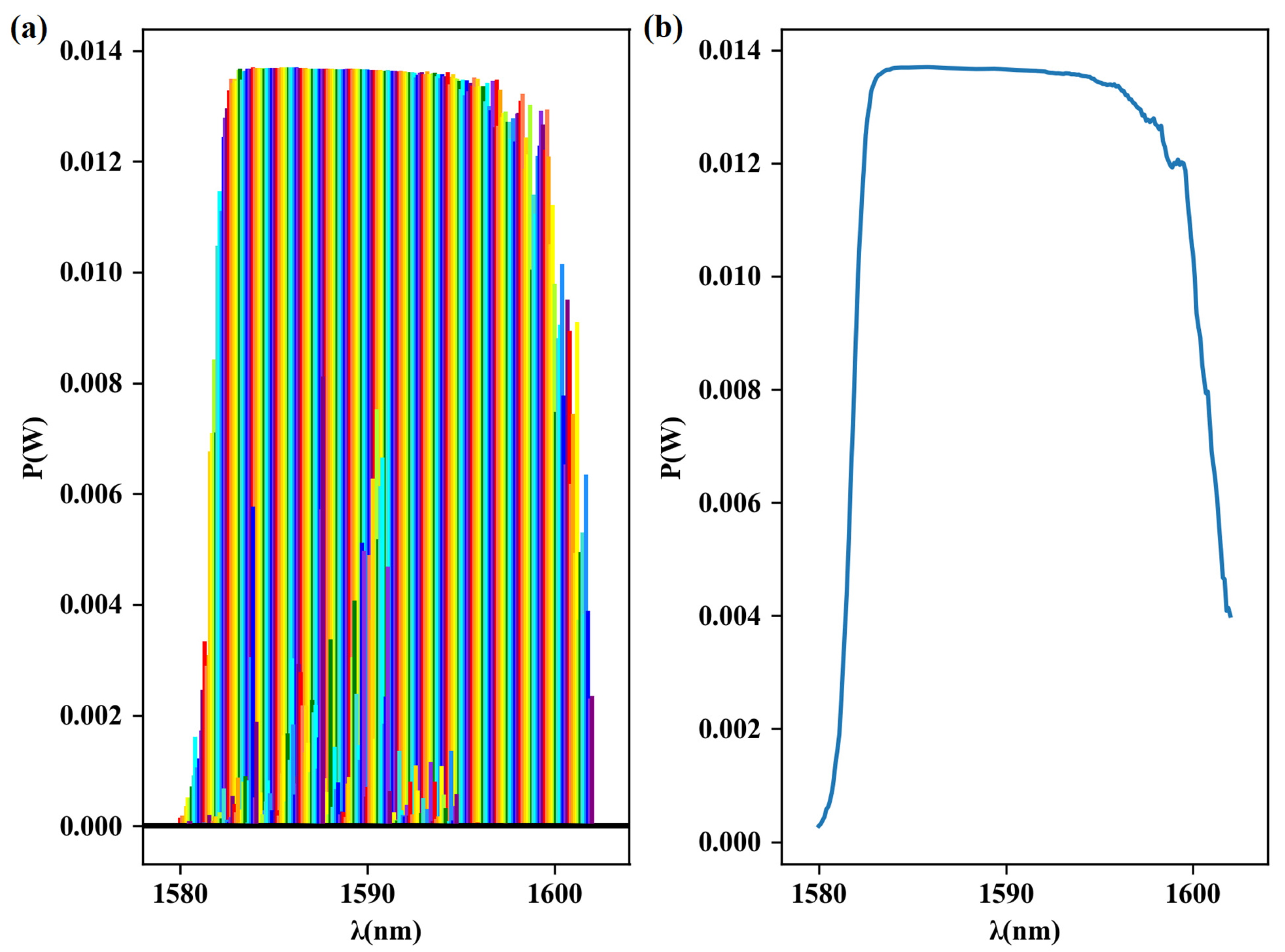
Figure 8 demonstrates that under the current parameters, the laser has a flat gain spectrum from 1583 nm to 1596 nm, which is important for designing tunable lasers to achieve specific functions. The gain spectrum at different wavelengths can be calculated using our model under different parameters.

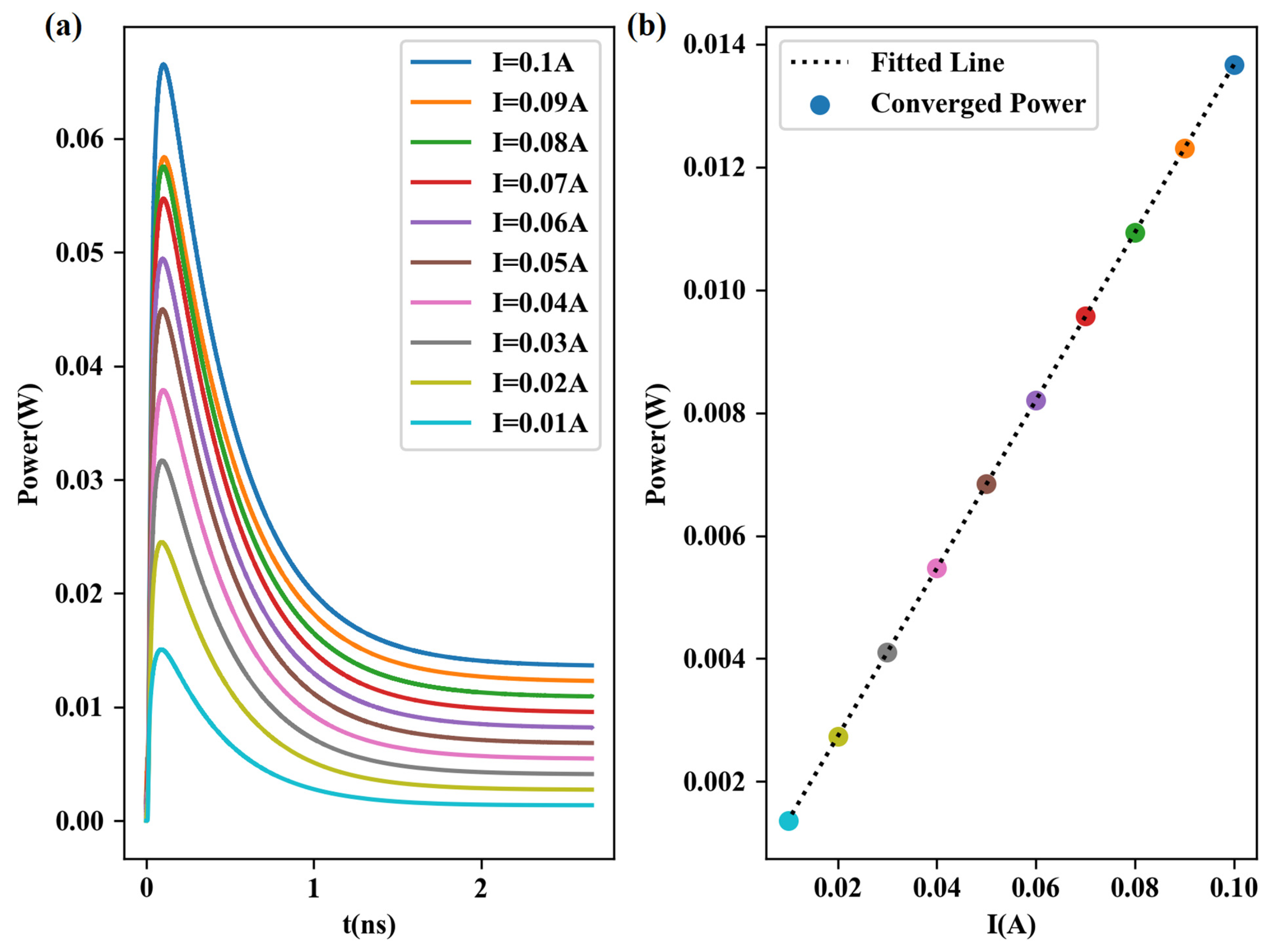
Figure 9a shows the convergence process of the output power under different injection currents, which is similar for different currents with rapid initial growth followed by slow decline and convergence. The convergence is determined by the gain spectrum at different carrier concentrations. Figure 9b indicates that the convergence results are linear for currents between 0.01 A and 0.1 A. The convergence process for different output wavelengths varies depending on its position on the gain spectrum and the injection current.

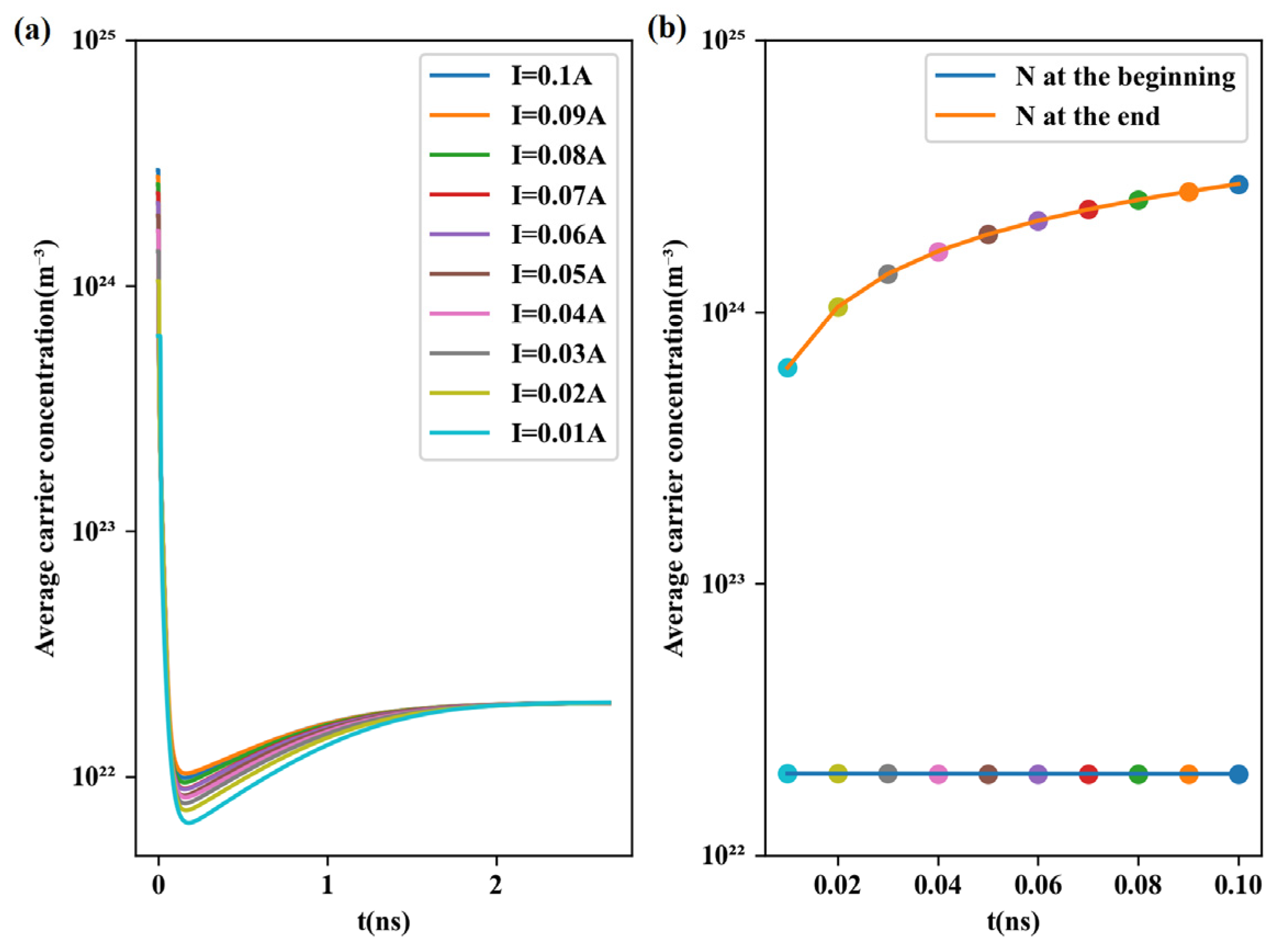
Figure 10a shows the convergence process of the carrier concentration at different injection currents, while Figure 10b indicates that the converged system gains are almost the same under different currents. In the steady state, a larger current produces more photons in the cavity, thus consuming more carriers in the gain region, which requires a larger current to supplement the consumed carriers.

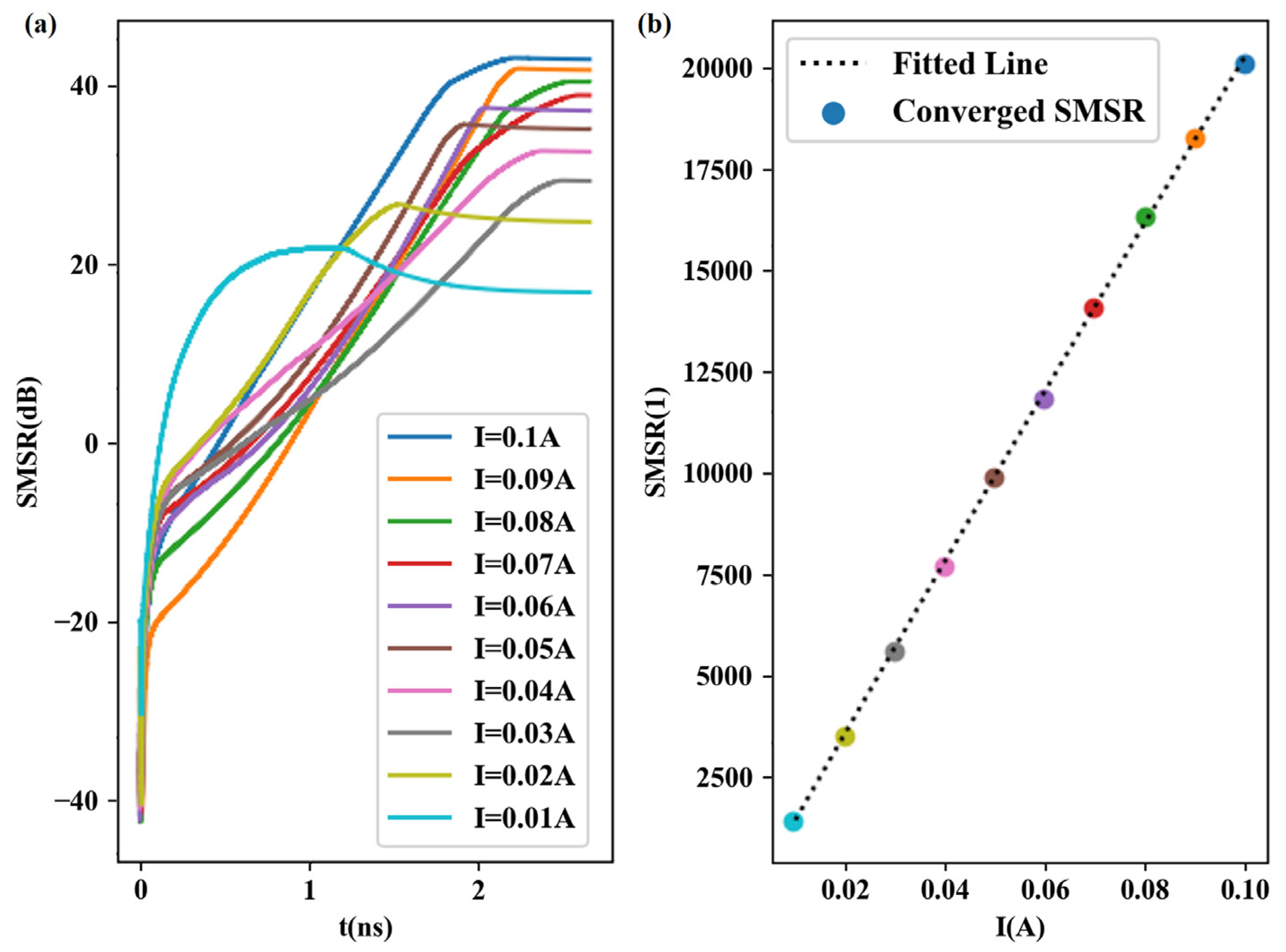
Figure 11 illustrates the convergence of the laser’s SMSR over time at various currents. In comparison to Figure 3, the laser output’s SMSR is two to three orders of magnitude higher than the SMSR of the transmission spectrum. This can be attributed to the gain region discussion, where the gain chip exponentially amplifies the light at each wavelength, consequently increasing the SMSR by several orders of magnitude. With all other conditions remaining constant, raising the current will solely enhance the power of the primary mode. Therefore, a linear relationship exists between the converged SMSR and current, as evident in Figure 11b.

In summary, this paper describes a model for simulating the behavior of a tunable laser based on a distributed feedback structure. The model takes into account the interaction between the optical field and carrier concentration in the active region of the laser, as well as the effects of various physical phenomena, such as gain clamping and mode competition. The simulation results show that the model can predict the behavior of the laser with high accuracy and provide insights into the underlying physical mechanisms involved. The model can also be used to optimize the design of tunable lasers for specific applications by calculating the gain spectra under different parameters.

6. Conclusions

This paper presents a comprehensive analysis of the operation and performance of a dual FP etalon-based ECTL. The paper provides insights into the effect of the tuning region on the phase modulation of light and proposes an idea for designing etalon FSR. Additionally, the paper uses the FDTW method to discuss the changes in the differential gain index of the gain region with the carrier concentration and analyzes the influence of laser injection current on various parameters, such as power, carrier concentration distribution, and SMSR. The theoretical model presented in this paper can provide a valuable reference for the design and optimization of ECTLs.