1. Introduction
Laser scanning is a topic that is extremely broad in scope. A scanning system can track objects by capturing reflected light or by fluorescing the image and acquiring the fluoresced light. The output system directs light to produce images for marking [
1]. Laser scanning capture technology has been widely studied and applied in many engineering fields due to its ability to accurately and directly scan small targets.
In the field of biology, the main applications of laser scanning capture include subcellular protein localization [
2], the imaging of biological surfaces [
3], trapping light-absorbing microparticles in the air [
4,
5], bright-field light microscopy [
6] and trapping nanoparticles on the surfaces of solutions [
7]. In the medical field, research and development on technologies such as laser capture microdissection [
8,
9], the laser capture of individual cells in complex tissues [
10], laser capture cell sampling [
11], the analysis of gene expression profiles using laser capture microdissection [
12], and the laser capture of blood cells [
13] has demonstrated that laser capture technology has profound significance for medical progress and for the treatment of major diseases. In the engineering field, laser scanning acquisition is mainly used in laser radar, mechanical engineering, the space industry, and other fields, such as 3D nanofabrication [
14], high angular resolution LiDAR [
15], super-resolution laser probing [
16], laser printing [
17], and laser scanning [
18,
19]. However, in actual engineering applications, the problems of environmental complexity and spatial instability exist, posing new challenges for laser capture and tracking systems.
This article focuses on the field of laser communication and conducts research on the capture of moving targets. The measurement of dim or small moving targets in complex environments calls for high sensitivity, high precision and high angular deflection velocity in the visual axis for traditional single-station measuring equipment. The laser tracking measurement system has been proposed as a new type of measurement system with high measurement accuracy, a wide measurement range, and high pointing accuracy, and has thus become a global research hotspot in target tracking technology.
The premise of maneuvering tracking is to establish an accurate target model and then, based on a variety of filtering tracking algorithms, effectively estimate the target’s position in the next step. Whether visual sensors or laser detection methods are used, target capture is the first step in the target tracking process.
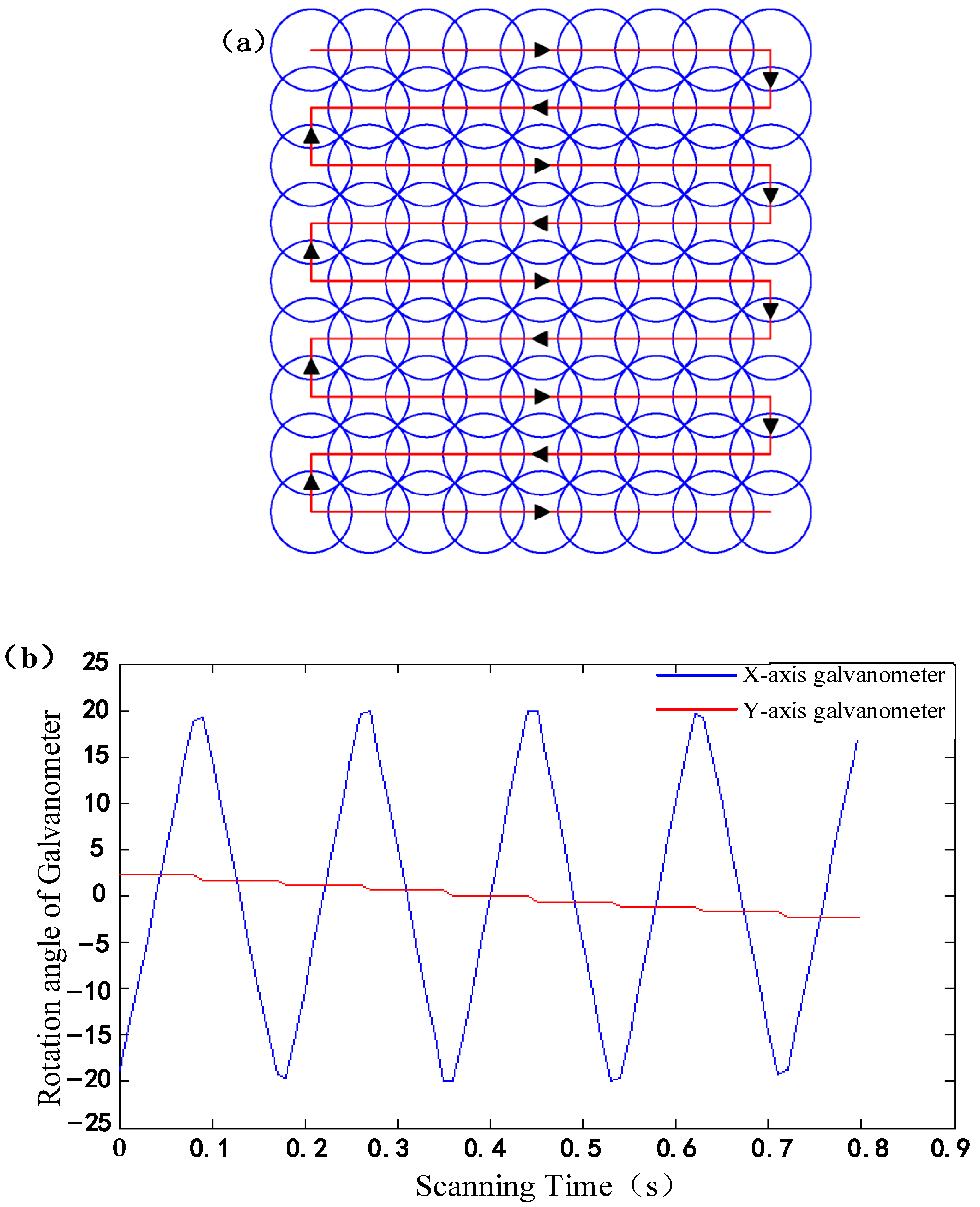
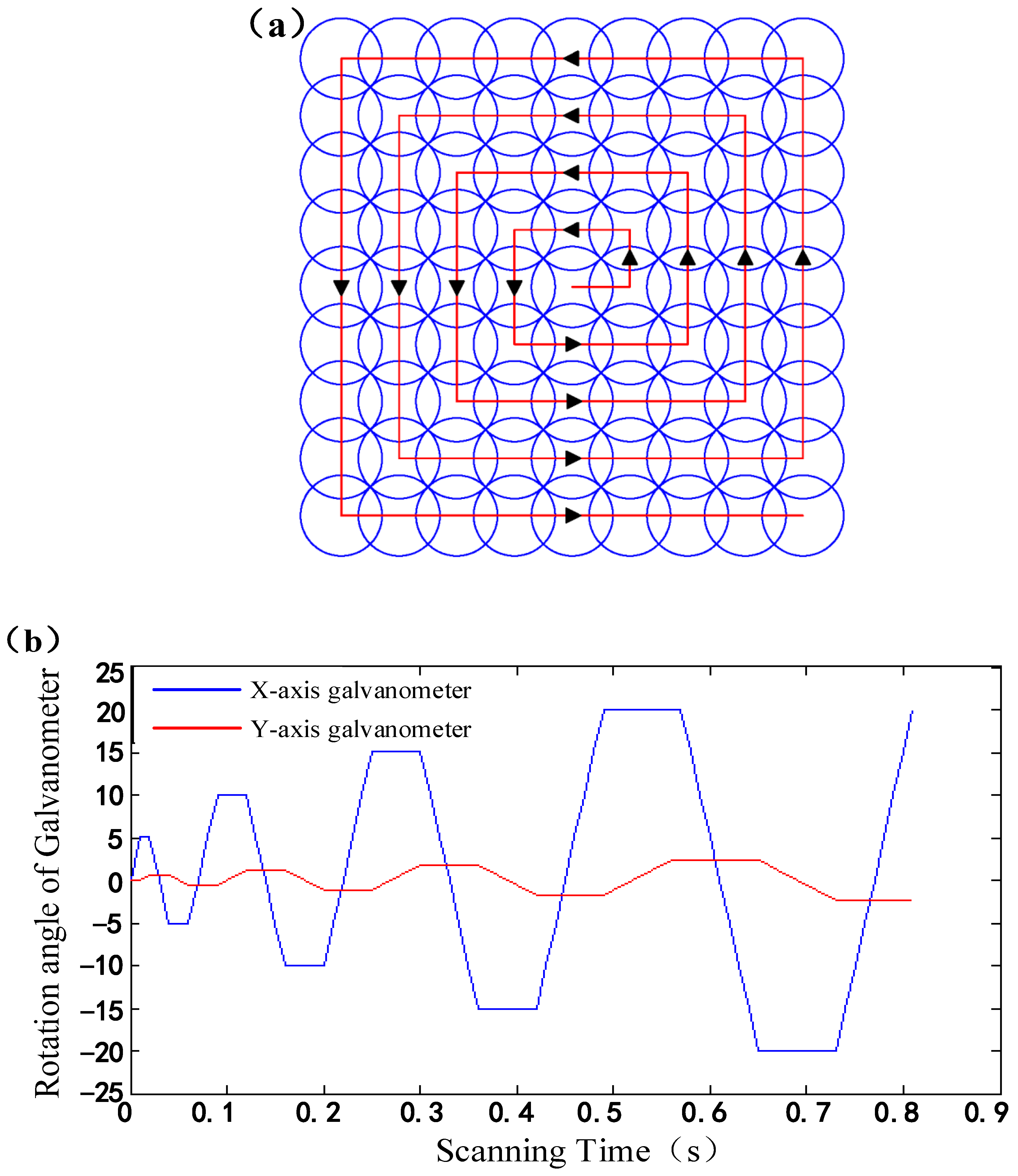
Common scanning methods in laser tracking systems include rectangular branch scanning, rectangular spiral scanning, circular spiral scanning, hexagonal spiral scanning, etc. These scanning methods are used in laser communication, satellite docking, airborne radar, and other fields. The scanning mode and scanning parameters used in a photoelectric detection system are of great significance when it comes to improving the detection accuracy, detection efficiency, and target acquisition probability of the laser tracking system. In previous studies, photoelectric scanning detection models played an important role in monitoring low, slow, and small targets in the air, enabling the efficient capture of moving targets [
20]. A rectangular spiral scanning method based on spiral scanning [
21] has been proposed for space rendezvous lidar target acquisition technology that simplifies the system’s structure, reduces system difficulty, and increases acquisition probability [
22]. In previous studies on the use of radar scanning in space laser communication, it was concluded that uniform sinusoidal spiral scanning has greater advantages [
23], but this scanning method has a complex control process for galvanometer laser scanning [
24,
25,
26]. In addition, some studies have compared several common scanning methods and found through theoretical analysis and simulation experiments that hexagonal spiral scanning has advantages that are different from those of other scanning methods [
27,
28]. When the moving target’s position is combined with a Gaussian distribution model, the capture probability using rectangular spiral scanning is 85.80%, and the required number of light feet is 81; the capture probability using rectangular branch scanning is 62.48%, and the required number of light feet is 81; and the acquisition probability using hexagonal spiral scanning is 87.79%, and the number of light feet required is 61. The acquisition speed of hexagonal spiral scanning is, therefore, the fastest.
The sampling frequency in laser tracking systems is also an important factor. When the sampling frequency of the target increases, the acquisition probability of hexagonal spiral scanning and rectangular spiral scanning increases steadily, and the acquisition probability of hexagonal spiral scanning is the highest out of all methods. Moreover, changes in the sampling frequency have a great impact on the rectangular branch scanning. Due to improvements in the sampling frequency, the branch scanning method starting from the edge can capture a moving target at the center of the field of view more quickly. If the laser sampling frequency is not high enough when the laser reaches the center of the field of view, the target will have moved outside of the field of view, that is, the acquisition probability will be extremely low. There is a peak before and after the sampling frequency reaches 30 kHz wherein the acquisition probabilities of hexagonal spiral scanning and rectangular spiral scanning show a certain decline. This indicates that when the sampling frequency increases, the spiral scanning spot moves faster to the edge of the field of view, resulting in a small reduction in the acquisition probability. The acquisition probability of rectangular branch scanning tends to be stable, indicating that it is not restricted by the sampling frequency but by the scanning method itself.
For a moving target with a high probability of appearing in the center of the field of view, the hexagonal spiral scanning mode and the target cannot be effectively matched in the time domain and space domain. Based on the above research, combined with the research background, this paper proposes an improved hexagonal scanning mode—called improved hexagonal honeycomb structure scanning—which establishes a prior motion model with a Gaussian distribution in the threshold scanning range. In the same scanning field of view, the acquisition probability is higher than that of traditional hexagonal spiral scanning.
2. Improved Scan Capture Model with a Hexagonal Honeycomb Structure
2.1. Establishment of the Improved Hexagonal Honeycomb Structure Scanning Model
At present, most hexagonal scanning methods available in the literature are hexagonal spiral scanning methods; the principle of this method is similar to spiral scanning and zigzag scanning [
29,
30,
31]. They all scan from the center to the 2π direction. Based on the research of [
20], it was concluded that when the position where the target enters the visual threshold range for the first time is modeled with a Gaussian distribution and different scanning methods are used to cover and determine the visual field, the hexagonal spiral scanning method has a higher acquisition probability than the circular and rectangular methods.
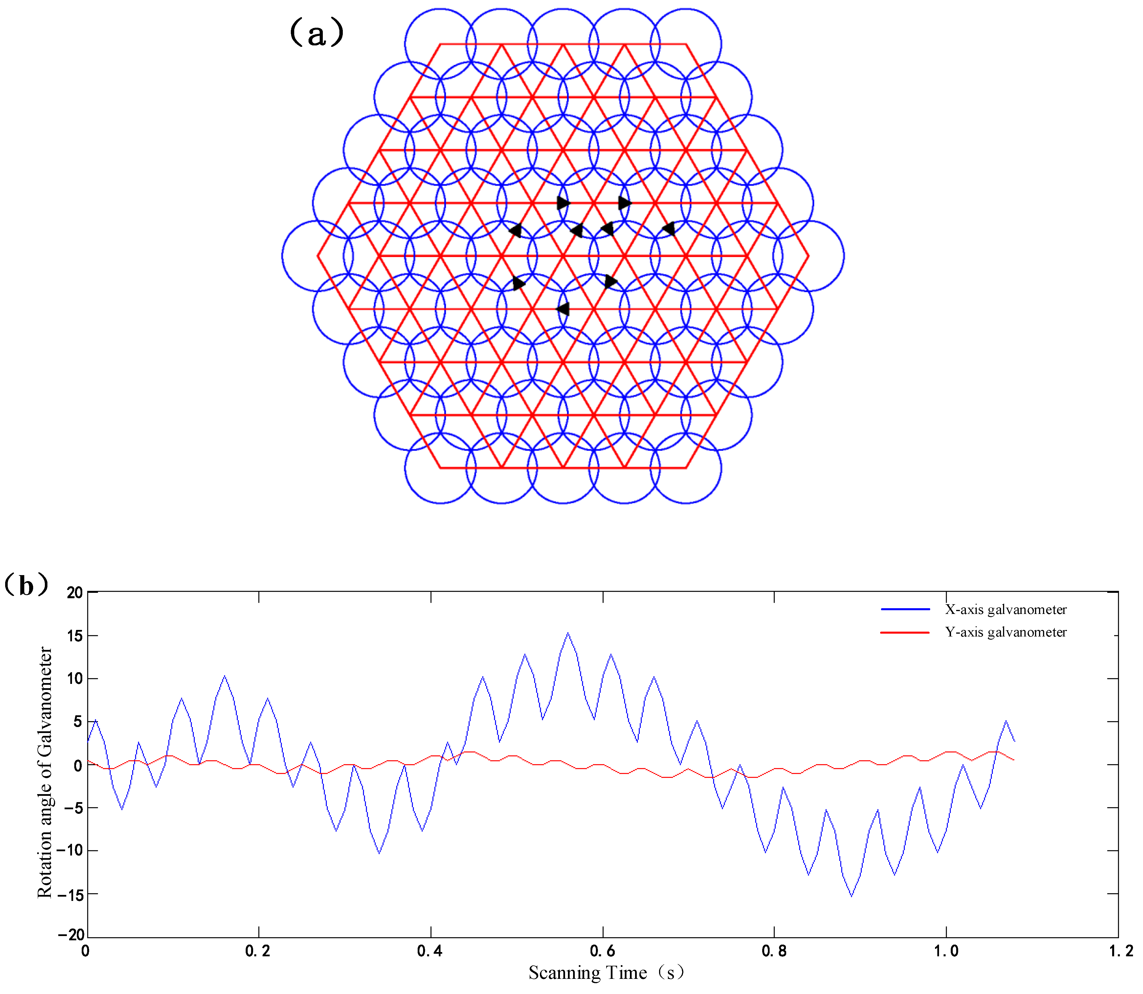
To further improve the target acquisition probability of laser tracking systems and make the detection spot appear in the center more often, this paper proposes a new hexagonal scanning method—the improved hexagon honeycomb structure scanning model. Different from traditional spiral scanning with an increasing hexagonal radius, the scanning of the hexagonal honeycomb structure is improved by first completing the hexagon of the smallest unit and then scanning from the inside to the outside. This method achieves detection in the center of the field of view more often and reduces the number of times target capture occurs outside the field of view. For moving targets with a Gaussian distribution, the scanning mode of the improved hexagonal honeycomb structure is the same as the spiral scanning mode, which starts scanning from the area with the highest probability of target occurrence. At the same time, this mode makes up for the defect of missing scanning of the outer circle of spiral scanning and can repeat the spiral scanning of the inner circle.
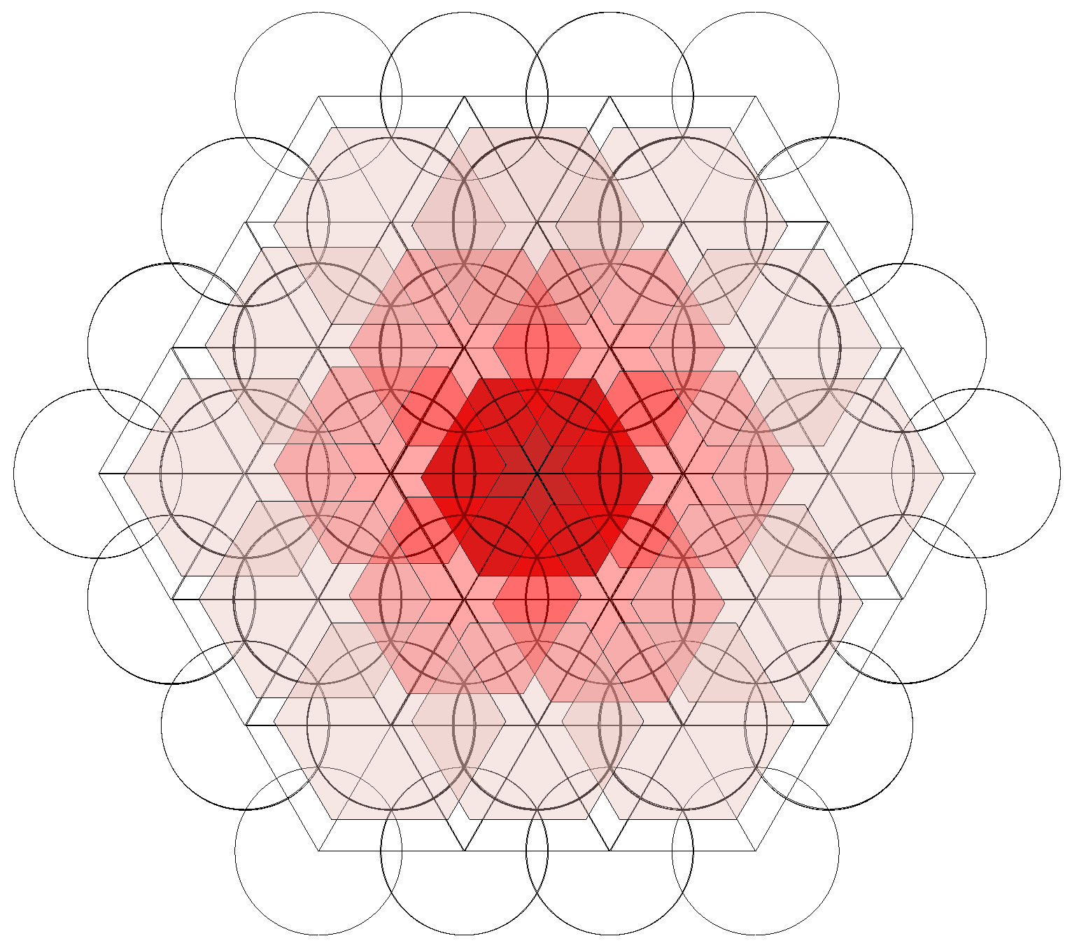
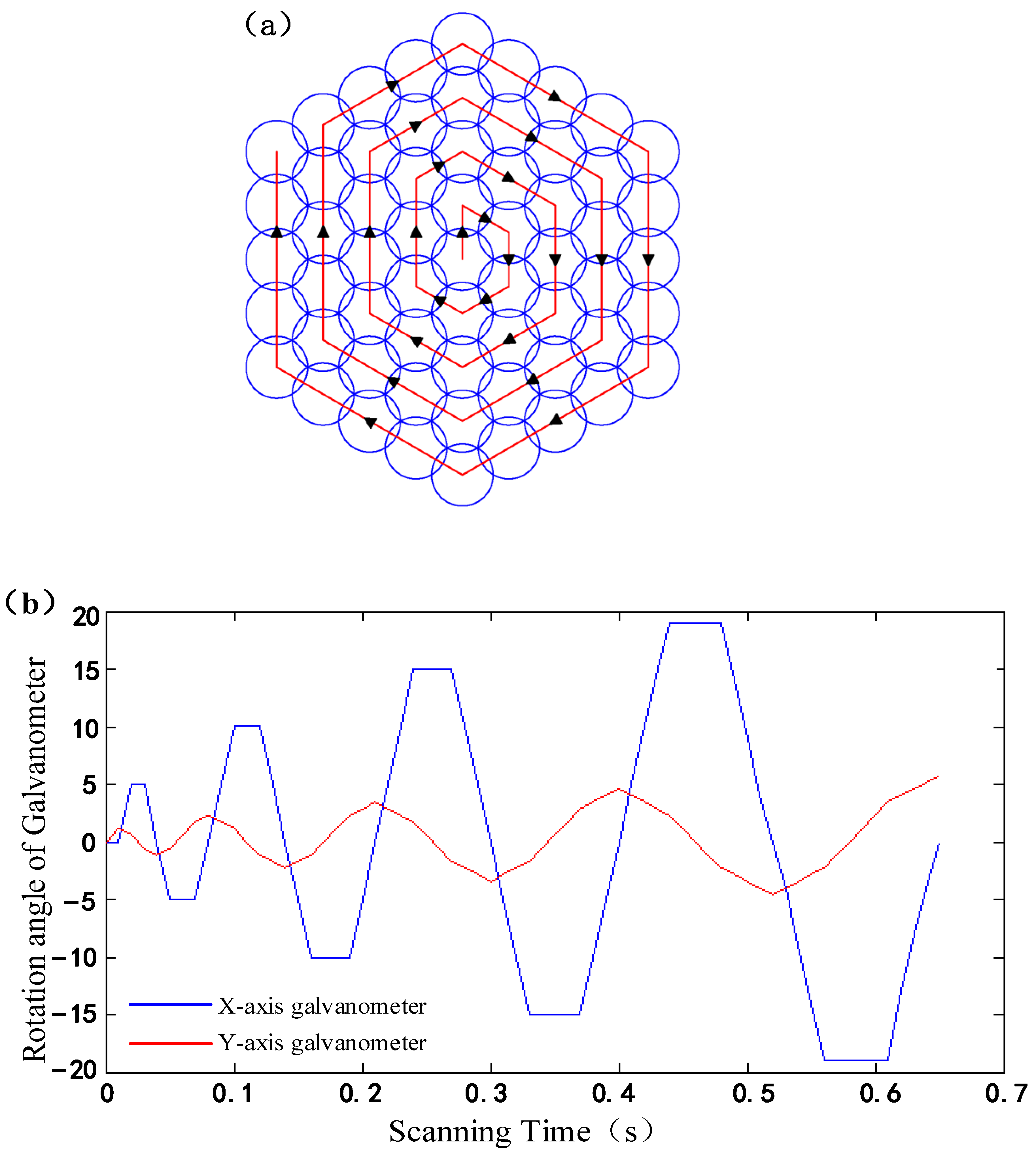
Assume that the pulse frequency matches the scanning frequency, that is, the laser sends out a pulse every time the galvanometer jumps. Then, define a visual scanning range threshold. The scanning mode is shown in
Figure 1. In the figure, a circle is used to represent the light foot generated by a pulse, and an overlapping hexagon is used to represent the path of the laser spot’s center. The darker the color, the more overlaps there are.
The scanning path of the improved hexagonal honeycomb structure is briefly described below:
- (1)
First, form a light foot at the origin at the center of the scanning field, then scan along the regular hexagon edge of the center to form the first layer of light feet with six vertices as the centroid;
- (2)
Take the vertex of the central regular hexagon as the centroid and make six regular hexagons. The scanning track is the edge of the six regular hexagons, scanning out the second layer of light feet;
- (3)
The apex of the hexagon is formed after the second layer of scanning, and the bisection points of each side are taken as the hexagon centroid. Its edges are scanned in turn to generate the third layer of light feet, and so on.
According to the scanning mode shown in the figure, it can be seen that the optical foot density and coincidence rate in the center of the field of view are higher. Under a normal distribution of the target and determination of the field of view’s size, compared with other scanning methods, the target is more likely to be captured using this scanning mode.
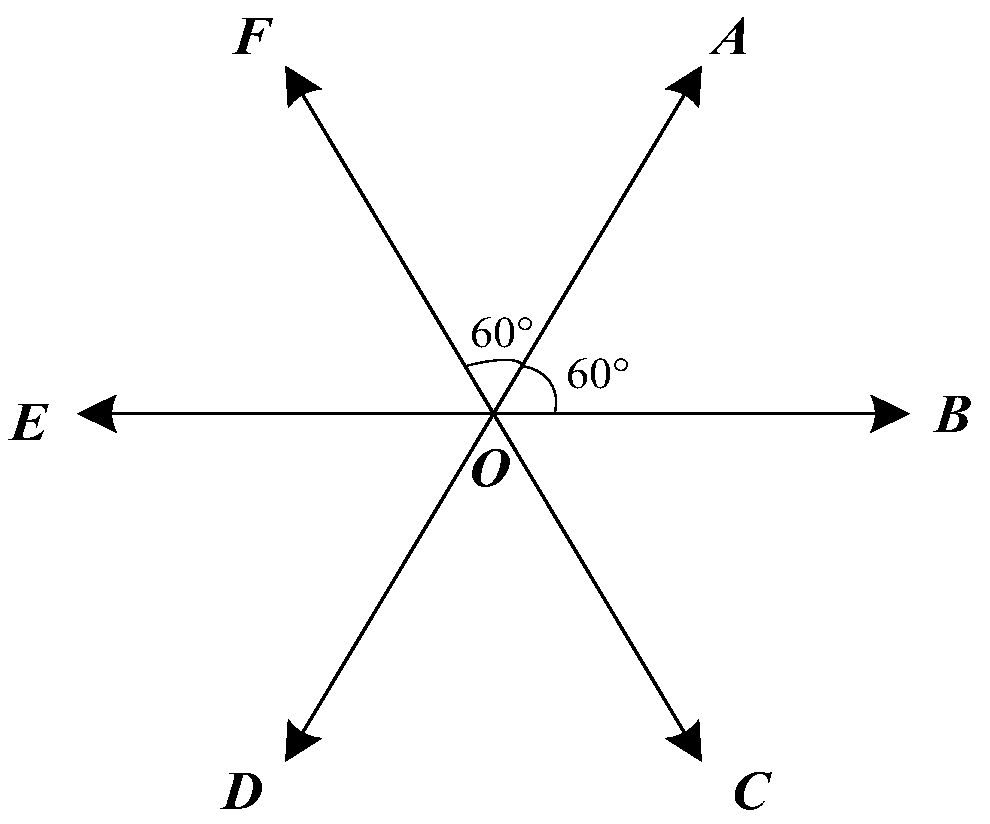
Therefore, the scanning path of the improved hexagonal honeycomb scanning structure is modeled. First, define the center position of the current flare. The vector groups A, B, C, D, E, and F of starting point O have included angles of 60° between their adjacent vectors, and the vectors’ lengths are equal to the side length of the regular hexagon of the path. The model is shown in
Figure 2.
The scanning path of the light spot is represented by a vector. If the included angle between the light foot and the horizontal right is 60° from the central position O of the light spot, and the length is r, it is represented by vector A. It can be seen that the scanning path vector satisfies the relationship of A = −D, B = −E, and C = −F. That is, if the trajectory follows the vector of A + B + C + D + E + F, and the light foot position returns to the starting point.
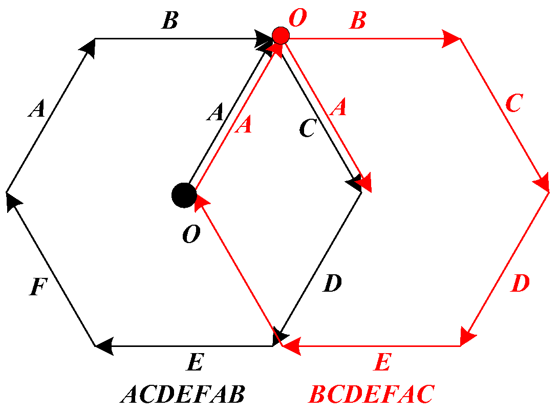
The scanning path vector of the first optical foot is shown in
Figure 3.
Starting from the origin O of the scanning field of view, the optical foot conducts a scan around O to obtain the first optical foot. Its path description vector is
A + C + D + E + F + A + B, abbreviated as ACDEFAB. From the above-mentioned path
A =
−D,
B =
−E,
C =
−F, the path description can be simplified to obtain the end position A of the optical foot relative to the origin after the path scanning as follows:
This process is shown in the black path in
Figure 3. Here, the accumulation of seven vectors is uniformly used to represent one regular hexagonal path scan, and the second regular hexagonal path scan is performed using the end position A of the first scan as the starting point. Then, the second path’s description vector is
B +
C +
D +
E +
F +
A +
C, abbreviated as
BCDEFAC, as shown in the red path in
Figure 3.
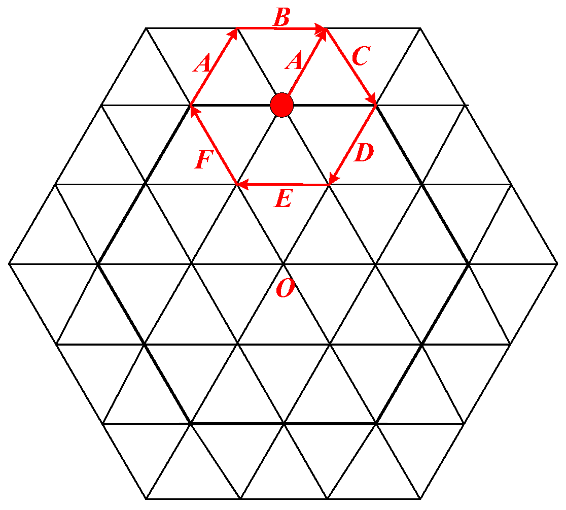
Table 1 shows the scanning path of the first optical foot.
In the table, the optical foot scanning path No. 0 represents the hexagonal path with the scanning field origin as the centroid. The optical foot scanning path from No. 1 to No. 6 is the scanning path of the first layer of optical feet. The starting point is marked with vector coordinates relative to the origin. The starting point position of the current serial number is the last ending point position, which can be obtained by adding the last starting point vector and the path description vector. For example, the starting point of track No. 2 is the coordinate of the
B vector, the path description vector is
CDEFABD, and the starting point method for finding the No. 3 track is (
Figure 4):
Table 2 shows the scanning track of the second optical foot.
Due to the different methods of selecting the starting point of the second layer scanning path, the path vectors with serial numbers 1 and 2 have special properties. The other path description vectors are the same as the path description vectors with serial numbers 2 to 6 in the first layer, and they cycle once at the hexagon bisection point. This path description vector is extended to the scanning path of the third layer, and the corresponding path description vector of the first layer is cycled three times at the outermost regular hexagonal trisection point to obtain the three-layer light foot scanning path.
2.2. Capture Conditions
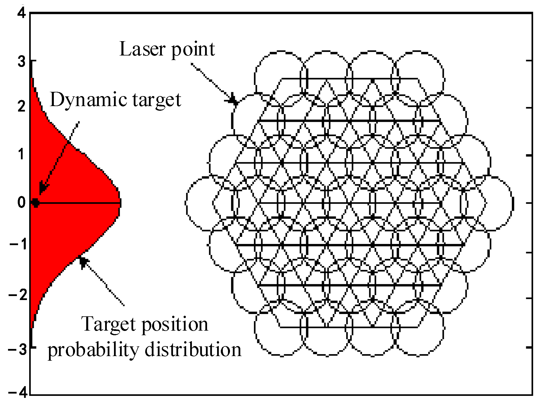
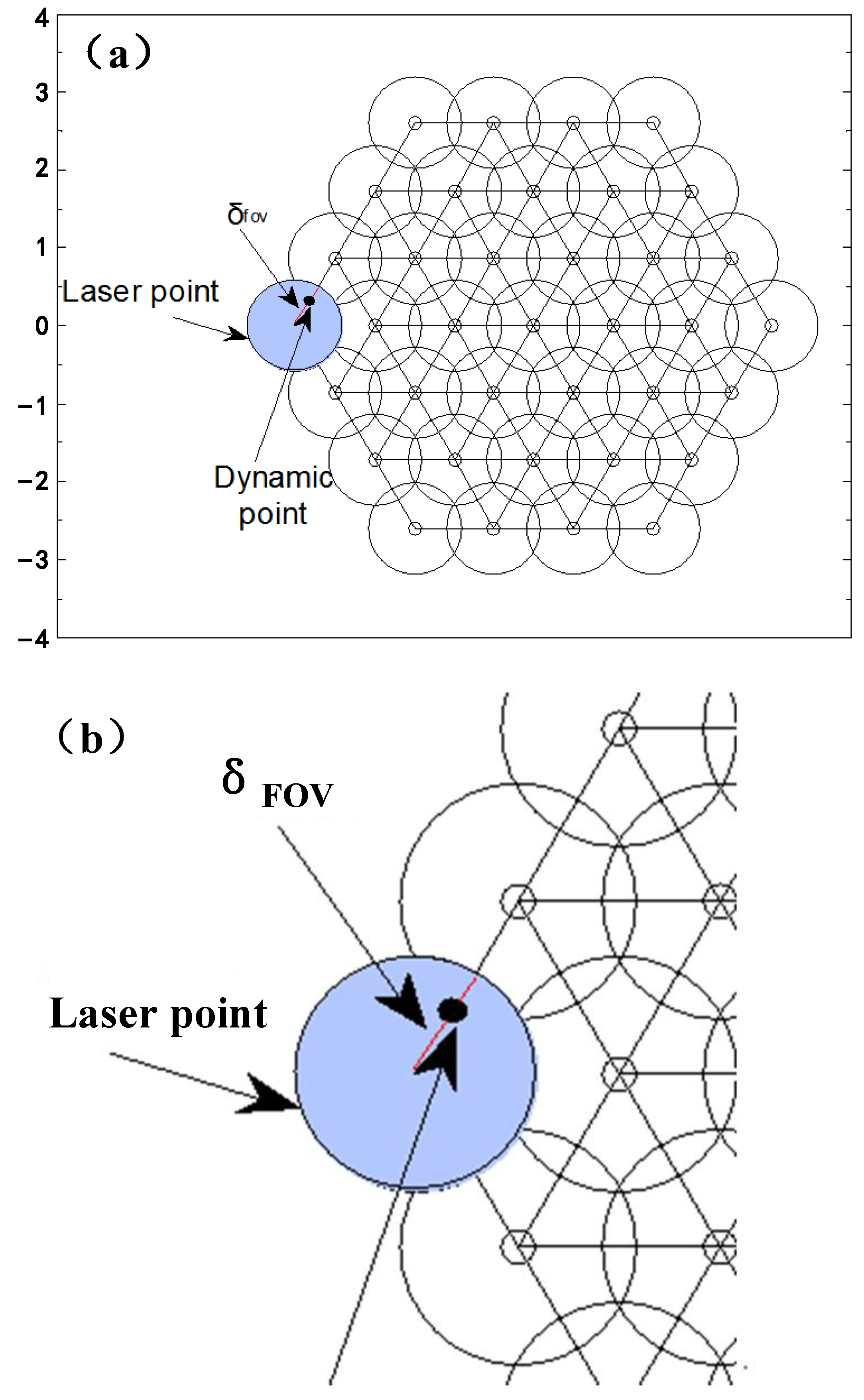
The controllable factors affecting the comprehensive probability of the laser tracking system capturing the target include the galvanometer scanning mode, the laser sampling frequency, and the laser divergence angle. The capture probability refers to the likelihood that the laser is scattered by the target and received by the receiving optical system within the laser’s single frame scanning area. As long as the signal is received, it is determined that the target is captured. After the target enters the field of view, appropriate scanning system parameters are selected to complete the target acquisition, so that the maximum probability of the target falling into the visual range of the receiving system is achieved. Acquisition systems using other working modes, such as microwave radar, can scan the detection airspace in all directions, without considering the scanning speed. The laser acquisition and tracking system of the TOF measurement system selected in this paper is based on the matching of the time sequence and space to complete target acquisition. Therefore, the need to model the two kinds of independent random processes of the target and scanning systems based on a time sequence must be considered in the simulation and verification process.
The capture diagram of a moving target and the proposed detection model are shown in
Figure 5, in which the measured target enters the detection area from the left side.
To simplify the complexity of the model, when a galvanometer-type photoelectric detection model is scanned for one frame, the time when the target enters the field of view is exactly the time when the detection model starts scanning; that is, the time when the random target enters the field of view and the time when the detection model scans for one frame are both T, which are set in the same detection area. When modeling a moving target, the following points should be obeyed:
- (1)
The target motion model is an inertial target model;
- (2)
The scanning field of view position is the best estimation prior result;
- (3)
The target time location in the two-dimensional plane is Gaussian white noise, that is, it obeys a Gaussian distribution;
- (4)
The noise in the z direction is not considered.
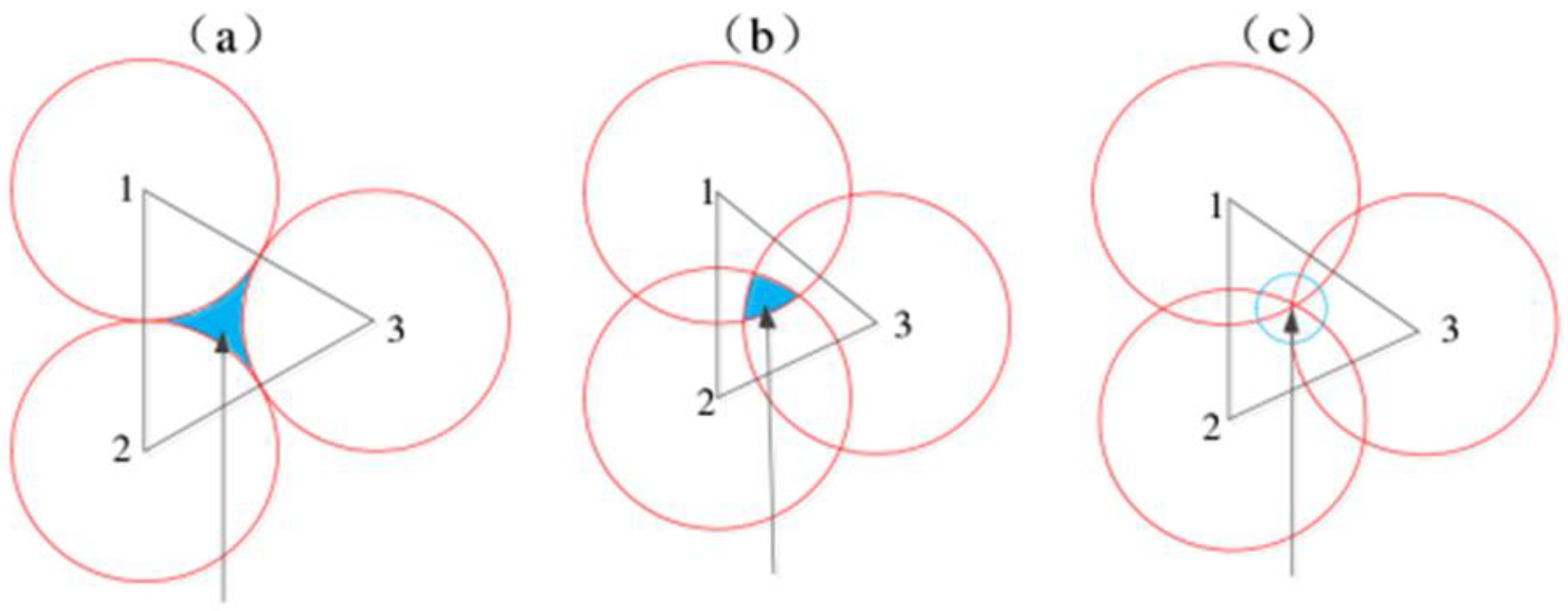
2.3. Scanning Step Size Analysis
During galvanometer scanning, the scanning point’s step size has a great impact on moving target acquisition. If the step size is too large, some scanning areas will be missed, reducing the acquisition probability, as shown in
Figure 6a. Too small a step size will increase the scanning repetition rate and capture time, as shown in
Figure 6b. To achieve fast and efficient scanning, the optimal scanning step size that completely covers the capture uncertainty area must be selected. The scanning beam can not only eliminate missed scanning areas but also reduce invalid overlapping scanning areas, as shown in the center circle of
Figure 6c.
The numbers in
Figure 6. represent the scanned light feet. When the points are tangent, a missed scan area in the blue area will appear in the middle, reducing the capture probability; When the points intersect, a repeating area with a blue part will appear in the middle, increasing the scanning time; When the centers intersect, the scanning efficiency is highest.
The projection of the laser light foot on the scanning area is shown in
Figure 7. Assume that the laser beam’s divergence angle is
, the laser spot’s diameter is
, and the step size of two adjacent spots is
. At this time, the light spot offset distance is
and
. When
is less than the maximum step size
, the laser spots overlap. Since
is of the order of mrad, the projection areas of two adjacent laser spots are regarded as circles with the same diameter. In rectangular spiral scanning, if the coverage area of the spot is rectangular, as shown in
Figure 7a, the scanning field of view is
S at this time:
Therefore, when and only when has the largest area of S, according to the scanning relationship, the step size of the scanning point is .
In hexagonal spiral scanning and hexagonal edge equidistant spiral scanning, the overlapping area of the light beam is small, as shown in
Figure 7b. At this time, the step size of the scanning point is
according to the scanning relationship.
4. Experimental Simulation
To verify that the improved hexagonal honeycomb structure scanning method can improve the capture times of moving targets, this paper uses the control variable method to carry out a simulation and comparative analysis of four scanning methods.
Let the moving target speed of the CV model be 100 m/s, the laser output frequency be 10 kHz, the laser beam divergence angle be 10 mrad, the spot diameter be 25 mm, the step lengths of rectangular scanning and rectangular spiral scanning be 1.66 mm, and the step lengths of hexagonal spiral scanning and hexagonal honeycomb structure scanning be 3.15 mm. The distance R between the defined target point and the laser detection center point satisfies the formula:
where
is a random number.
When the target is captured successfully, the spatial relationship between the photodetector and the target is shown in
Figure 12, and the distance
R between a single optical foot and the target point within the scanning threshold meets the following requirement:
where
is the receiving field angle of the target detector, and
is the plane distance between the target and the scanning visual threshold.
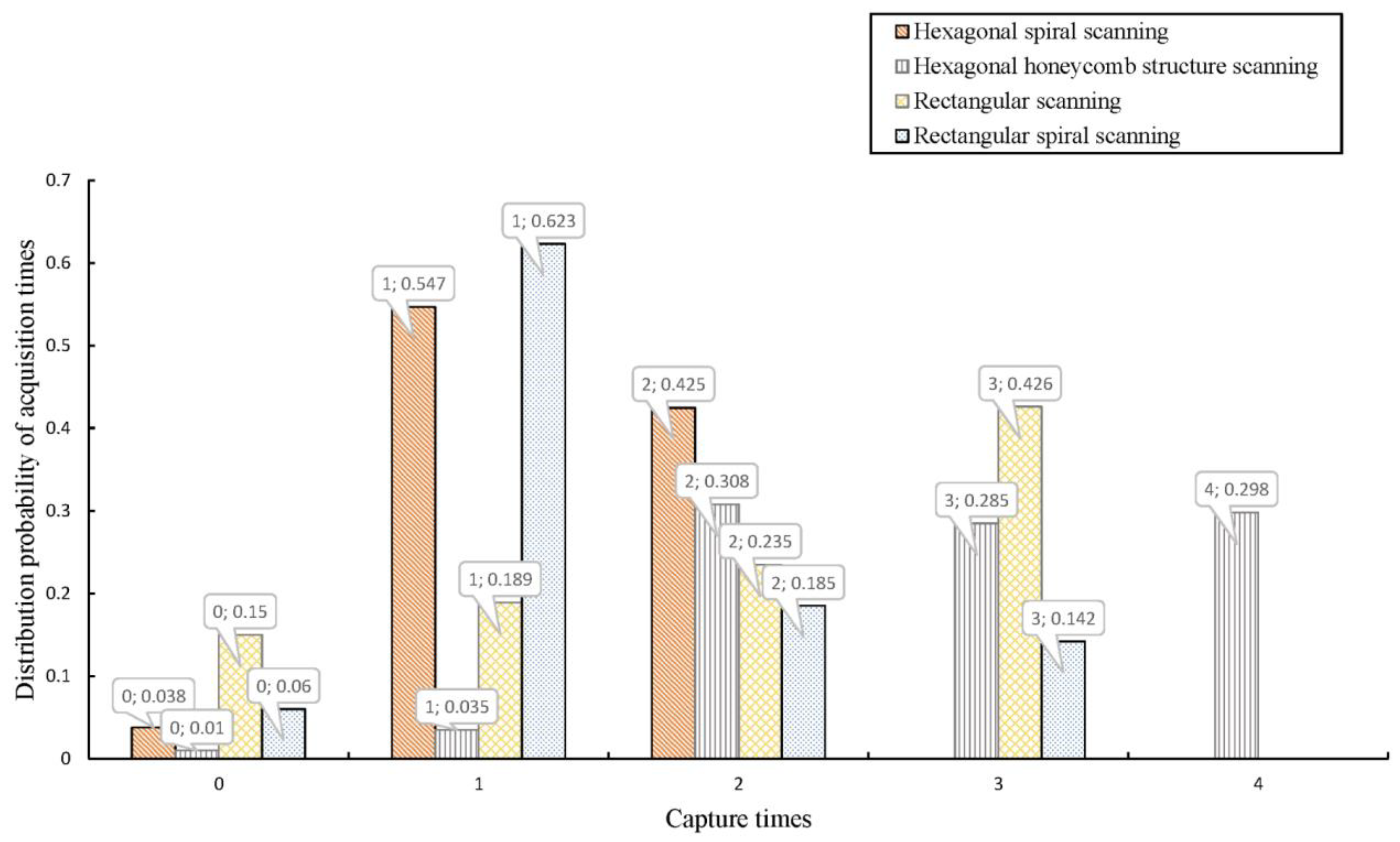
Matlab Simulink simulation software was used to establish simulation models for the four scanning methods; Monte Carlo simulations were used for capture analysis; 1000 single field scans were conducted for each scanning method; and the proportion of single field scanning capture times of each scanning method to the total scanning times was output.
The acquisition results obtained after the simulation are shown in
Figure 13. From the simulation results in
Figure 13, it can be concluded that when the target has been scanned 1000 times in a single field, the proportion of moving targets being captured by traditional hexagonal spiral scanning one to two times is large, 0.547 and 0.425, respectively. One moving target being captured by rectangular spiral scanning accounts for a large proportion, of 0.623. The proportions of two to three mobile targets being captured by rectangular branch scanning are 0.235 and 0.426. The proportion of two to four mobile targets captured by the improved hexagonal honeycomb structure scanning is larger, being 0.308, 0.285, and 0.298. The proportion of targets not captured after scanning a frame is smaller than that of other models. It can be seen from
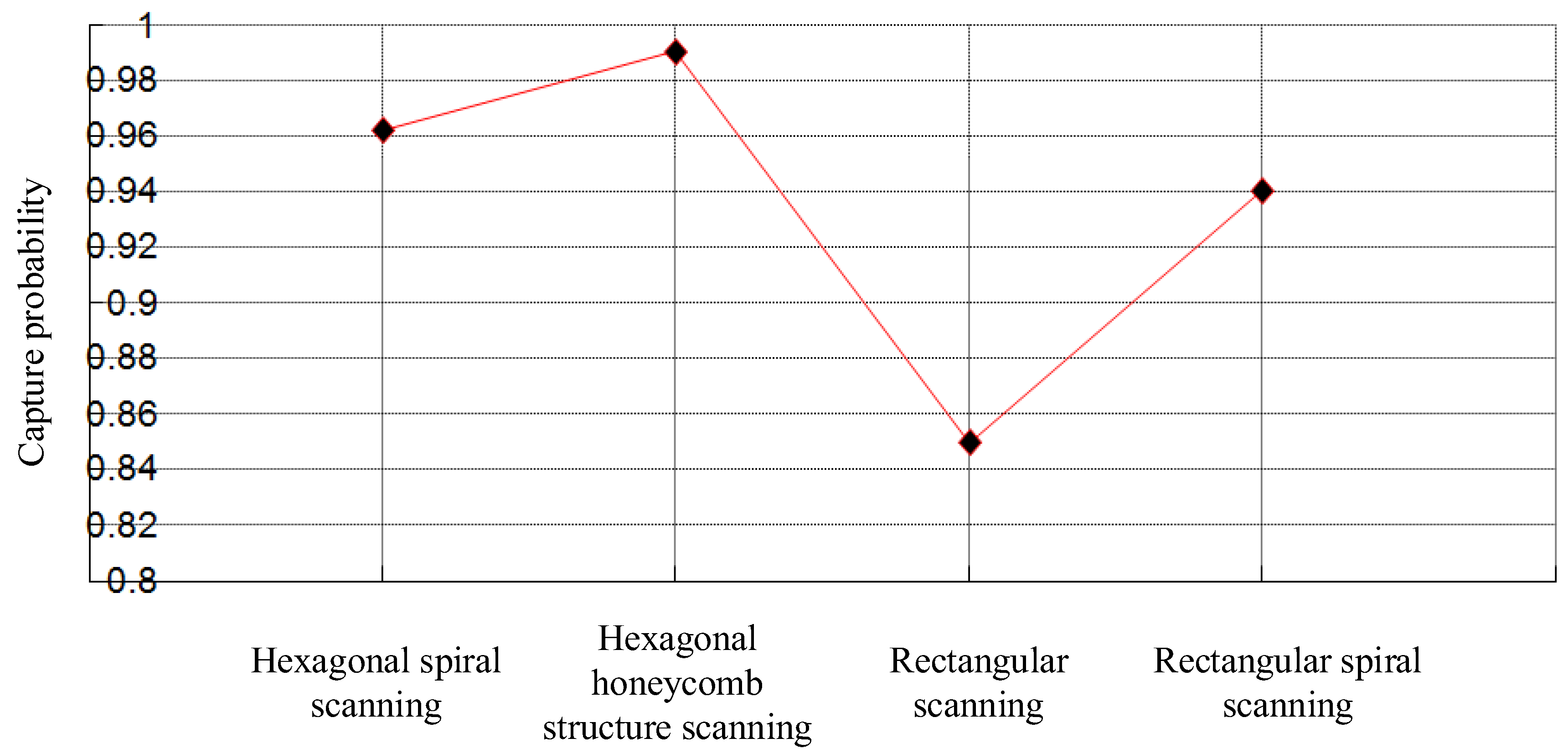
Figure 14 that when a target enters a fixed field of view, it is captured when it is detected more than or equal to one time. The maximum acquisition probability of the improved hexagonal honeycomb structure is 99%, followed by the hexagonal spiral scan at 96% and the rectangular spiral scan at 94%. The minimum acquisition probability is obtained by the rectangular branch scanning method, at 85%.
When 1000 experiments were conducted, 988 were successfully captured, the probability of target capture in each experiment was
p = 0.9888, and the probability of success was 98.88%. According to the binomial distribution, 988 obeyed the binomial distribution with parameters of 1000 and 0.9888, the sample average was
. Calculate the confidence interval with normal distribution: assuming the confidence level is 95%, the
, the standard deviation of the sample is
. The formula for the confidence interval is:
The confidence interval obtained through calculation is [0.9822, 0.9953].


