Article

Mie Scattering Nanointerferometry for the Reconstruction of Tightly Focused Vector Fields by Polarization Decomposition

1
School of Optical-Electrical and Computer Engineering, University of Shanghai for Science and Technology, Shanghai 200093, China
2
Zhangjiang Laboratory, Chinese Academy of Sciences (CAS), 100 Haike Road, Shanghai 201204, China
3
Shanghai Key Lab of Modern Optical System, University of Shanghai for Science and Technology, Shanghai 200093, China
*
Author to whom correspondence should be addressed.
Photonics 2023, 10(5), 496; https://doi.org/10.3390/photonics10050496
Submission received: 23 March 2023 / Revised: 13 April 2023 / Accepted: 21 April 2023 / Published: 26 April 2023

Abstract

:
Tightly focused vector fields, which can be generated by focusing a light beam through a high-numerical-aperture objective, play an important role in nano-optics research. How to fully characterize this kind of field in the subwavelength scale is a challenging but important task. The Mie scattering nanointerferometry technique has been proposed to reconstruct the tightly focused vector field accurately. In this work, we theoretically demonstrate that the technique can be realized by collecting the transmitted light with two orthogonal polarization states simultaneously. Therefore, when nanoparticles are employed to scan the fields to be measured, more information of the scattering field can be acquired in the far field. This is helpful for solving the linear inverse scattering problem by reducing the number of scanning points, thus making the measurement more efficient.

1. Introduction

In the research field of the interaction between light and nanoscopic objects, the enhanced field in the near-field region can be obtained at certain frequencies, which is also known as optical resonance [1]. Assisted by optical resonance, many interesting properties of objects can be observed more easily, such as fluorescence emission [2,3], Raman scattering [4], bound states in the continuum (BIC) [5,6], anapole states [7,8], and nonlinear optical effects [9,10]. These resonances are closely related to the optical properties of the nanoparticles, which should be well-designed and fabricated as required. In recent years, tightly focused vector field has been intensively studied, because many special states in nanoparticles can be excited under the illumination of such fields. Moreover, it has been shown that they also have great potential in the fields of optical storage [11], super-resolution microscopy [12], nano-fabrication [13], and optical micro-manipulation [14].
In recent decades, several techniques have been proposed to characterize the spatial distribution of tightly focused vector fields, including the knife-edge method [15,16], fluorescence film method [17], nanoscale fluorescence probe scanning method [18], field scanning optical microscopy [19,20], etc. The knife-edge method records the power of the transmission light by moving the knife edge, and the intensity distribution near the focus can be mapped. The method based on fluorescence thin film can indirectly measure the shape and size of the focus. By employing a nanoscale fluorescence probe, the optical field is scanned to reconstruct the three-dimensional intensity distribution of the focused light field by using the relationship between the intensities of the fluorescence signal and the illumination field. Near-field scanning optical microscope (NSOM) technology can also provide the intensity distribution of the measured field. However, distributions of phase and polarization are difficult to measure using the above methods. In 2014, T. Bauer et al. proposed a Mie scattering nanointerferometry technique [21] to measure the spatial distributions of the amplitude, phase, and polarization state of a tightly focused vector field by using a nanoparticle probe to scan the optical field. It has been demonstrated that the tightly focused fields by linearly polarized, radially polarized, and azimuthally polarized beams can be well reconstructed. Furthermore, the technique has been applied to measure the special light field distribution [22], study the transverse spin of unpolarized light [23], and develop super-resolution optical microscopy [24]. On the other hand, studying the interaction mechanism between light and Mie particles will help us to explore new physical phenomena. For example, the upper limit of circular dichroism can be achieved at a specific frequency by using light excitation of anapole states in chiral nanospheres [7]. The nonlinear optical properties of a single Mie particle are used to detect the magnetic components of a light field with arbitrary electromagnetic structures [25]. By observing the Mie scattering of a single superconducting particle in the superfluid helium quadrupole magnetic field, the angular distribution of the scattered light intensity is used to determine the radius of the particle [26]. The Mie scattering nanointerferometry technique can be employed to experimentally study the properties of Mie particles excited by a vector field.
In this work, we theoretically propose a modified scheme for a Mie-scattering nanointerferometry technique which decomposes the transmitted light according to the polarization directions and reconstructs the incident field based on the distributions of intensity and polarization of the transmitted light. Specifically, the incident field is scanned by the nanoparticle probe, and during the scan process, x-polarized and y-polarized light distributions at the pupil plane of the collection objective are recorded. By the polarization decomposition method, more restraint conditions for the tightly focused field can be obtained. Considering the light field is highly concentrated near the focal point, it is suitable to be expanded by the vector spherical harmonics (VSHs). The light scattering process is rigorously solved by the T-matrix method. The relationship between the expansion coefficients and the x- and y- polarized components of the transmitted field has been built. Therefore, the number of restraint conditions is doubled compared with the previous work, which only collects the patterns of the total transmitted field. This polarization decomposition method can reduce the spatial scan points, while the restraint conditions are still sufficient to solve the linear inverse problem. In fact, the measuring time of this technique mainly depends on the scan process. Therefore, our work can speed up the reconstruction of the tightly focused vector light fields.

2. Theoretical Model

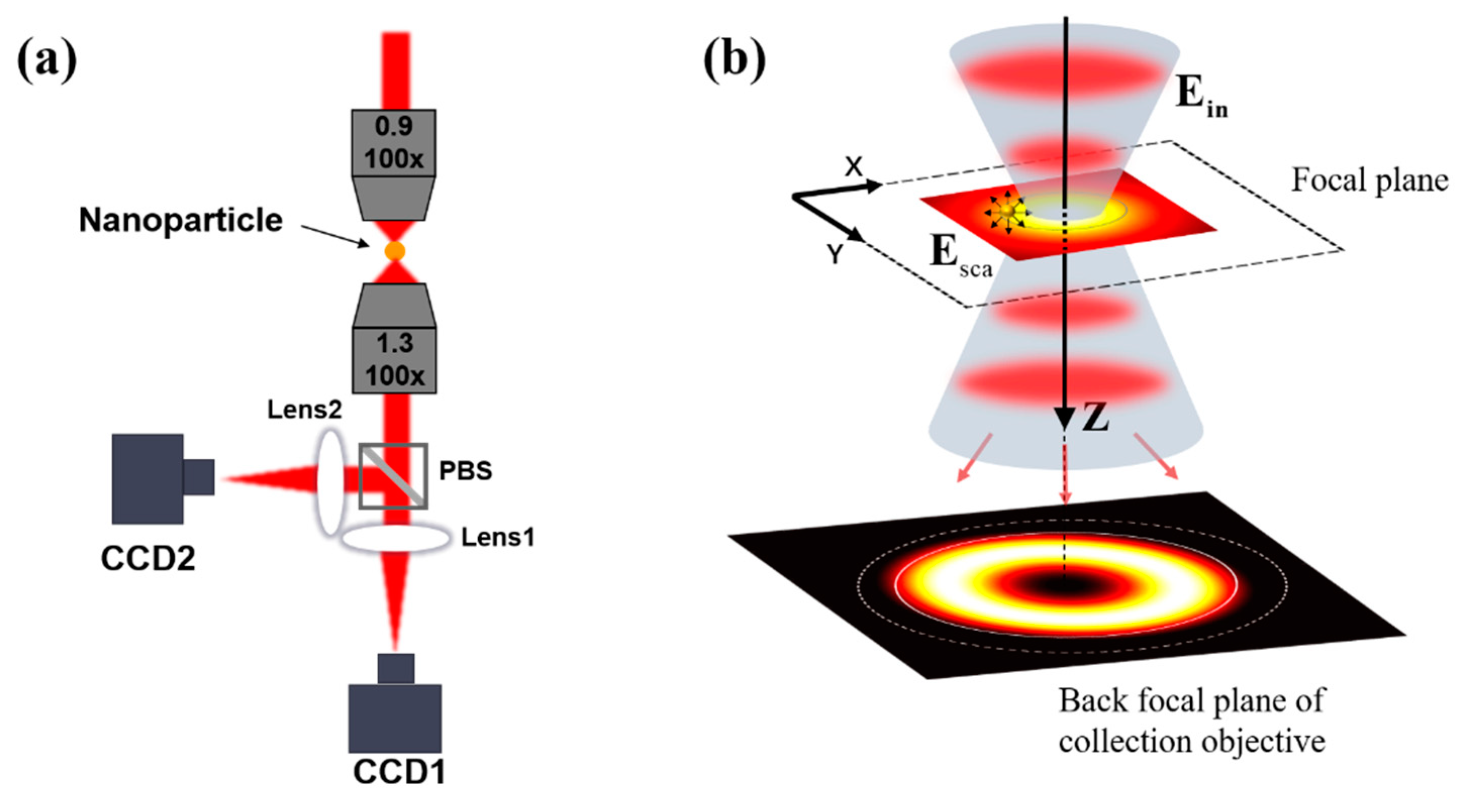
The scheme for the proposed method is shown in Figure 1a. The incident beam is focused by the upper high-NA objective. In the tightly focused vector field, a nanosphere can produce the scattering field. Then, the combination field of the scattering field and the incident field is collected by the lower objective with a larger numerical aperture than the upper one. The polarization beam splitter (PBS) is used to decompose the transmitted beam according to the polarization directions. Therefore, the x- and y-polarized components of the transmitted beam are detected by CCD1 and CCD2, respectively. Lens1 and Lens2 are used to transfer the light field at the pupil plane of the collection objective on the image planes of CCD devices. During the measurement, the nanosphere is used to spatially scan the tightly focused vector field on the focal plane (z = 0) as shown in Figure 1b. The scan is carried out to fully acquire information on the scattering field, which is enough to reconstruct the incident field. To determine the relationship between the measured field and the intensity patterns recorded by CCD cameras, we next solve the scattering process to study the dependence of the incident field on the intensity patterns. In this case, these measurable patterns can be considered as the constraint condition of the incident field. Finally, the incident field can be determined by solving the inverse scattering problem.
In order to use nanoprobes to reconstruct the full vector field of tightly focused beams, the scattering process should be analyzed rigorously. For the nanosphere particle, the Lorenz–Mie theory is suitable for calculating the scattering field. In this theoretical frame, the incident field and the scattering field outside the nanosphere are both expanded by vector spherical harmonics (VSHs) in Equations (1) and (2)
E in = n = 1 m = n n u m n Rg M mn k 0 r + v m n Rg N mn k 0 r ,
E sca = n = 1 m = n n a m n M mn k 0 r + b m n N mn k 0 r .
where k0 is the wave vector in free space and r = (r, θ, ϕ) represents the location of the field point and the origin of the spherical coordinate is at the center of the nanosphere. It should be noted that the incident field is expressed as the summation of regular VSHs, which have finite value at the origin, while the scattering field contains only outgoing VSHs to guarantee the radiation boundary condition in the far field. The order of VSH is denoted by (m, n). When the expansion coefficients (i.e., umn and vmn) are determined, the task of field reconstruction has been completed. The expression in Equation (1) is also called Whittaker angular spectrum expansion, which is regarded as an efficient method to represent the tightly focused vector field with wavelength-scale volume [27].
Following the notation of reference [28], the regular VSHs can be expressed as:
R g M mn = γ m n j n ( k r ) i π n m θ ^ τ n m ϕ ^ e i m ϕ ,
R g N mn = γ m n n ( n + 1 ) k r P n m ( cos θ ) e i m ϕ r ^ + γ m n ψ n ( k r ) k r τ n m θ ^ + i π n m ϕ ^ e i m ϕ .
where jn(kr) represents the spherical Bessel function, P n m ( cos θ ) is the associated Legendre function, and ψn is the Riccati-Bessel function. γmn is a coefficient which only depends on the order of VSH.
γ m n = 2 n + 1 n m ! 4 π n n + 1 n + m ! 1 / 2 .
The θ-dependent functions of π n m and τ n m are expressed as:
π n m = m P n m cos θ sin θ ,
τ n m = d P n m cos θ d θ .
According to the Lorenz–Mie theory, the scattering coefficient (i.e., amn and bmn) can be calculated by the incident field, i.e., a , b T = T u , v T . The T is a diagonal matrix, which can be determined by the size and optical constants of the sphere. The diagonal matrix elements Taa and Tbb are represented as:
T a a = Z 0 ψ n k 0 R s ψ n k 1 R s Z 1 ψ n k 1 R s ψ n k 0 R s Z 1 ψ n k 1 R s ξ n k 0 R s Z 0 ξ n k 0 R s ψ n k 1 R s ,
T b b = Z 0 ψ n k 1 R s ψ n k 0 R s Z 1 ψ n k 0 R s ψ n k 1 R s Z 1 ξ n k 0 R s ψ n k 1 R s Z 0 ψ n k 1 R s ξ n k 0 R s ,
where ξ n ( x ) = x h n ( 1 ) x , h n ( 1 ) x represents the spherical Hankel function, ξ n ( x ) and ψ n ( x ) represents the derivatives of ξ n ( x ) and ψ n ( x ) , respectively, and Z0 and Z1 are wave impedance in free space and sphere, respectively. When the measured field is scanned by the nanosphere, the center of the nanosphere deviated from the origin of the coordinate. By employing the translation transformation rule [29], the effective T-matrix associated with the nanosphere position should be expressed as:
T e f f R 0 = T r R 0 T T r R 0 .
where R0 is the displacement vector, which is also the location of the nanosphere center. The transformation matrix T r R 0 can be obtained using the addition theorem of VSHs. Therefore, the transmitted field can be calculated analytically at each scan step by modifying the effective T-matrix of nanosphere. In the far-field region, the angular-dependence power of the transmitted light P ( θ , ϕ ) is contributed by both incident field and scattering field. It has been derived that P ( θ , ϕ ) is expressed as the summation of incident, scattered, and extinct power, where the extinction power here is caused by the interference between the incident and scattered fields, which has the same expression as the extinction term of Mie theory. The relevant derivation process is shown in Appendix A. Furthermore, on the pupil plane of the collection objective, P ( θ , ϕ ) can be decomposed by x- and y-polarized components as expressed as:
P x ( θ , ϕ ) = P i n ( x ) ( θ , ϕ ) + P s c a ( x ) ( θ , ϕ ) + P e x t ( x ) ( θ , ϕ ) ,
P y ( θ , ϕ ) = P i n ( y ) ( θ , ϕ ) + P s c a ( y ) ( θ , ϕ ) + P e x t ( y ) ( θ , ϕ ) .
In Equations (11) and (12), each part of the power can be calculated by the expansion coefficients of incident field and scattering field. Considering the relationship of a , b T = T e f f R 0 u , v T , one can theoretically calculate the far-field distribution of the light power as follows:
P x / y ( θ , ϕ ) = 1 2 Re u * v * w 11 ( x / y ) w 12 ( x / y ) w 21 ( x / y ) w 22 ( x / y ) u v .
Here, the w-matrix is determined by the conversion efficiencies between spherical harmonic functions and plane waves towards the directions of (θ, ϕ). The expression of w(x/y) matrix is:
w ( x / y ) = w i n ( x / y ) + T e f f * T w s c a ( x / y ) T e f f + T e f f * T w e x t ( x / y ) + w e x t ( x / y ) T e f f .
The (mn, mn′) elements of the w i n ( x / y ) are given in Equations (15)–(22):
w i n , 11 ( x ) = i n n γ m n γ m n 4 k 0 2 Z 0 π n m π n m cos 2 ϕ + i π n m τ n m π n m τ n m cos ϕ sin ϕ + τ n m τ n m sin 2 ϕ e i m m ϕ ,
w i n , 12 ( x ) = i n n γ m n γ m n 4 k 0 2 Z 0 π n m τ n m cos 2 ϕ + i τ n m τ n m π n m π n m cos ϕ sin ϕ   + τ n m π n m sin 2 ϕ e i m m ϕ ,
w i n , 21 ( x ) = i n n γ m n γ m n 4 k 0 2 Z 0 τ n m π n m cos 2 ϕ + i π n m π n m τ n m τ n m cos ϕ sin ϕ + π n m τ n m sin 2 ϕ e i m m ϕ ,
w i n , 22 ( x ) = i n n γ m n γ m n 4 k 0 2 Z 0 τ n m τ n m cos 2 ϕ + i π n m τ n m π n m τ n m cos ϕ sin ϕ + π n m π n m sin 2 ϕ e i m m ϕ ,
w i n , 11 ( y ) = i n n γ m n γ m n 4 k 0 2 Z 0 π n m π n m sin 2 ϕ i π n m τ n m π n m τ n m cos ϕ sin ϕ + τ n m τ n m cos 2 ϕ e i m m ϕ ,
w i n , 12 ( y ) = i n n γ m n γ m n 4 k 0 2 Z 0 π n m τ n m sin 2 ϕ i τ n m τ n m π n m π n m cos ϕ sin ϕ + τ n m π n m cos 2 ϕ e i m m ϕ ,
w i n , 21 ( y ) = i n n γ m n γ m n 4 k 0 2 Z 0 τ n m π n m sin 2 ϕ i π n m π n m τ n m τ n m cos ϕ sin ϕ + π n m τ n m cos 2 ϕ e i m m ϕ ,
w i n , 22 ( y ) = i n n γ m n γ m n 4 k 0 2 Z 0 τ n m τ n m sin 2 ϕ i π n m τ n m π n m τ n m cos ϕ sin ϕ + π n m π n m cos 2 ϕ e i m m ϕ .
where Z0 is the wave impedance in free space. The scattered multipole modes (Mmn and Nmn) and incident multipole modes (RgMmn and RgNmn) have different radial behavior. However, according to the plane wave expansion of VSH [21], the scattered multipole modes are just two times larger than that of the incident ones in far field. It can be determined that w s c a ( x / y ) = 4 w i n ( x / y ) and w e x t ( x / y ) = 2 w i n ( x / y ) . By using Equations (13)–(22), the angular distributions of the transmitted light intensities, P x ( θ , ϕ ) and P y ( θ , ϕ ) , can be calculated for the specific incident field denoted by u v T . In the setup in Figure 1a, P x ( θ , ϕ ) and P y ( θ , ϕ ) are measurable parameters. To reconstruct the incident field, the inverse problem of Equation (13) should be solved. Each measured transmitted light intensity can be considered as a constraint condition, which corresponds to a quadratic equation. During the scan process, the effective T-matrix depends on the position of the nanosphere on the focal plane. The number of constraint conditions (i.e., quadratic equations) is proportional to the number of scan points. In this work, the two orthogonal polarization states are separately analyzed, so the number of quadratic equations is doubled compared with the case that transmitted light are measured without polarization decomposition. The new variables of F l = Re A m n A m n * and G l = Im A m n A m n * (here, the Amn is either umn or vmn in the coefficient of expansion) are introduced to transform the nonlinear quadratic equations into linear equations with the form of WX = Y. When W is a full rank matrix, Fl and Gl can be obtained directly by solving the linear equations. Then, the complex expansion coefficients (i.e., umn and vmn) are determined by the gradient descent algorithm based on the value of Fl and Gl. Finally, the tightly focused field is reconstructed by Equation (1). In the next section, we will consider the reconstruction of the optical field, which is generated by tightly focusing a radially polarized beam.

3. Results and Discussions

In this section, we will discuss the reconstruction process for the light field which is generated by tightly focusing a radially polarized (RP) beam. The RP beam is a typical vector light field with non-uniform distribution in spaces of polarized states, which can be generated by the superposition of orthogonally polarized Hermite–Gauss modes [30]. An RP beam has an axially symmetric polarization structure in which the electric field is polarized along radial directions within the transverse plane. In cylindrical coordinates with r = ρ , ϕ , the field of an RP beam in paraxial approximation can be expressed as:
E ρ , ϕ = E 0 ρ w 0 e ρ 2 w 0 2 e i m 0 ϕ ρ ^ ,
where w0 is the beam waist and E0 represents the electric field amplitude factor. When the topological charge is zero (i.e., m0 = 0), using the Richards–Wolf diffraction integral theory [31,32], the tightly focused field near the focus point (ρ = 0 and z = 0) can be calculated using Equation (24) [15]:
E ( ρ , φ , z ) = k f e i k f 0 θ max g θ J 1 ( k ρ sin θ ) cos θ n ^ ρ 0 i J 0 ( k ρ sin θ ) sin θ n ^ z e i k z cos θ sin θ d θ ,
where Jn(x) is the Bessel function of the first kind with order n, f is the focus length of the upper objective, and k is the wavevector in free space. θ m a x = 1.12 , according to the sine condition, ρ = f sin θ . Thus, the apodization function can be expressed by g θ = β 0 e β 0 2 cos θ with β 0 = 1.25 
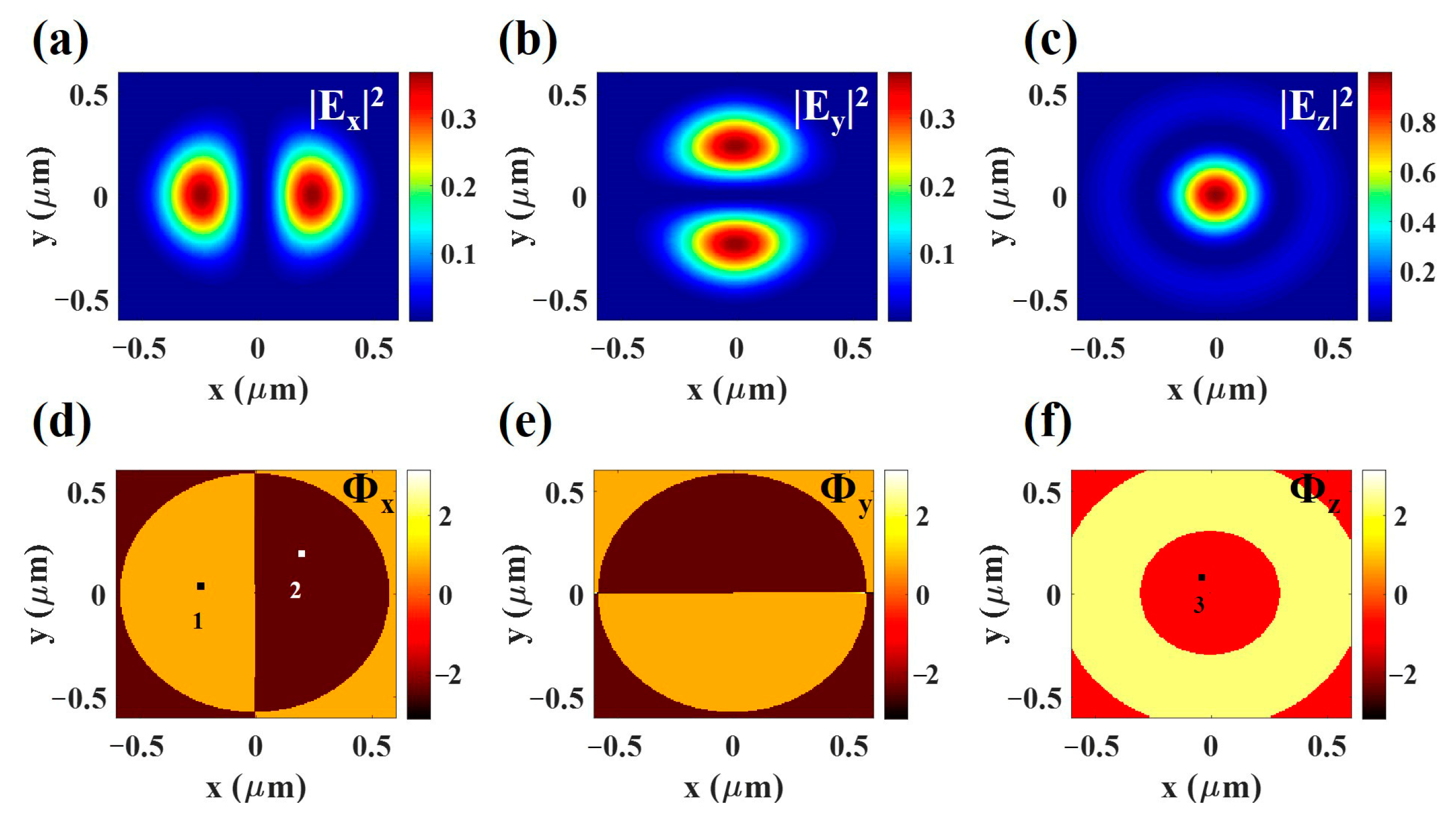
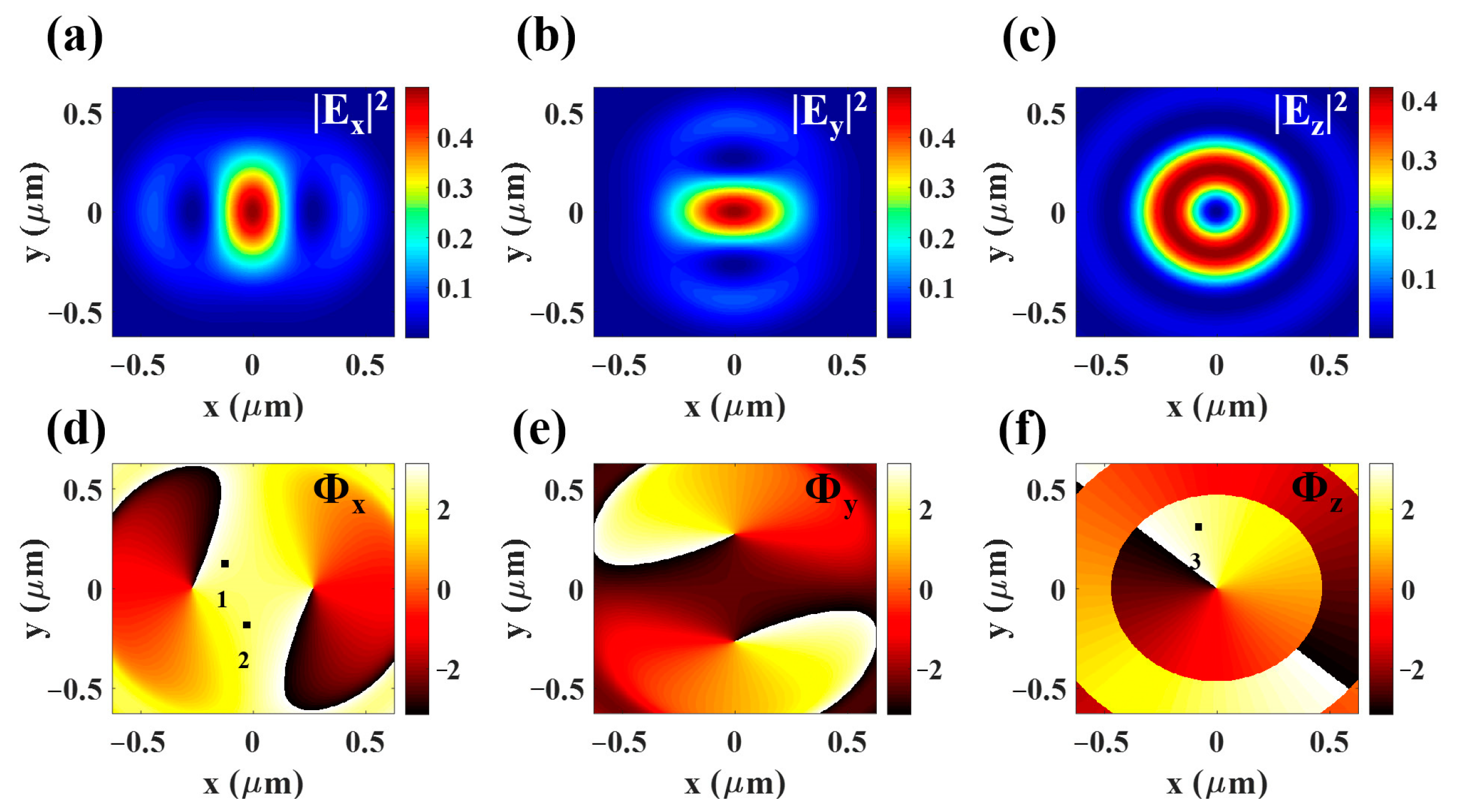
. The distributions of the three electric field components in the focal plane (z = 0) are calculated as shown in Figure 2. The distributions of |Ex|2, |Ey|2, and |Ez|2 are shown in Figure 2a–c. The light field travels in the direction of the z-axis, thereby causing the phase to vary along the z-direction. On the focusing plane (z = 0), the profile of the wavefront is flat. Due to the presence of a polarization singularity point at the center of field, there is a π phase difference between the light fields at two points related to origin symmetry, resulting in their oscillation directions being opposite. Among these three components, |Ez|2 is stronger than the other two transverse components and highly localized near the focus point [33]. This feature of RP beam enables it to generate a smaller focusing spot than linearly polarized or circularly polarized light. Therefore, the tightly focused RP beam can be widely used in microscopic imaging [34], optical trapping [35], and laser machining [36]. How to completely characterize this kind of light field is crucial to developing these applications.
Next, we will demonstrate the reconstruction process for the tightly focused field in Figure 2 based on measurable quantity in far field, i.e., the intensity pattern of the transmitted field through a nanoparticle in this method. To verify the feasibility of phase retrieval for different electric field components, three reference points are picked arbitrarily. The phase difference between each two points is ϕ1 − ϕ2 = π, ϕ1 − ϕ3 = 0.5π and ϕ2 − ϕ3 = −0.5π. In this model, the gold nanosphere is employed as the probe, whose radius is 40 nm, and dielectric constant is ε
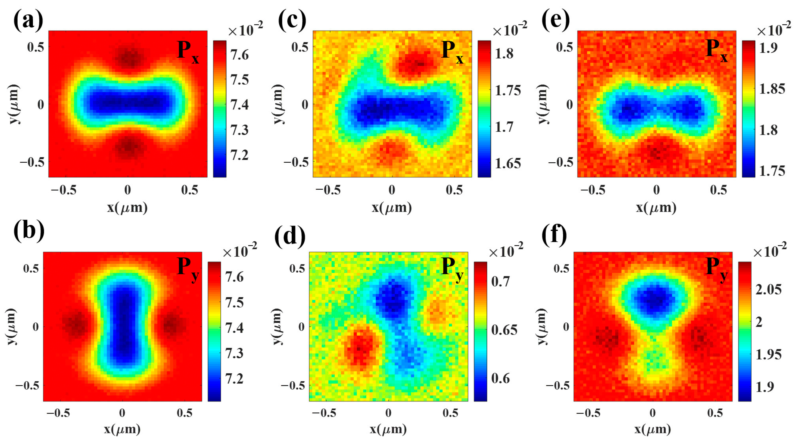
Au = −3.3915 + 2.3668i. The entire scan range is 1.25 μm × 1.25 μm and the scan step is 25 nm. Thus, 5000 images were recorded for the intensity pattern of the two polarization states at different nanosphere positions. To validate the feasibility of our method in experiments, we introduced random noise into each intensity image during the reconstruction process simulation. Specifically, we added random noise with a signal-to-noise ratio (SNR) of 15 dB to the intensity image, which is a typical value for commercial CCD cameras. As the noise from different pixels is independent, we addressed its impact by integrating the intensity values within specific regions on the CCD image plane. This approach effectively mitigated the influence of noise. The integrations mean to collect the angular-dependent transmitted power P x / y ( θ , ϕ ) within the corresponding solid angle Ω. When the angular integration region is θ θ 1 , θ 2 and ϕ ϕ 1 , ϕ 2 , the integrations are expressed as:
P x s u m Ω = θ 1 θ 2 sin θ d θ ϕ 1 ϕ 2 P x θ , ϕ d ϕ ,
P y s u m Ω = θ 1 θ 2 sin θ d θ ϕ 1 ϕ 2 P y θ , ϕ d ϕ .
When the integration region is θ 0 , 0.92 and ϕ 0 , 2 π , the light power of P x s u m and P y s u m is calculated when the nanosphere reaches each scan point as shown in Figure 3a,b. Although the integration region has cylindrical symmetry, according to Equations (14)–(21), the polarization decomposition method can break the symmetry and introduce more cross terms between two VSHs with different orders. Therefore, the rank of the equation system is increased, which is beneficial for the field reconstruction by solving the inverse problem. In Figure 3c–f, sector integration regions are adopted with θ 0 , 0.92 and ϕ 0 , 1 for Figure 3c,d, and θ 0 , 0.64 and ϕ 0 , 3 for Figure 3e,f. Furthermore, it is necessary to increase the number of equations by selecting more different integration regions, until the full-rank matrix is obtained for the equation system. To avoid the overlap between different regions, the areas of the integration regions become smaller, which will heighten the impact of noise and diminish the precision of the reconstructed field. In this work, 14 integration regions were selected to determine the constrained conditions for the measured field. When reconstructing a field using only the distributions of total intensity (i.e., sum of P x s u m and P y s u m ) under the same conditions, the coefficient matrix for the inverse problem may not be full-rank, thereby requiring more scanning steps and integration regions to attain enough constraint equations. However, using the polarization decomposition technique can provide more constrained conditions in the Mie scattering nanointerferometry method, making it particularly suitable for reconstructing complex light fields with a significant number of multipole modes.
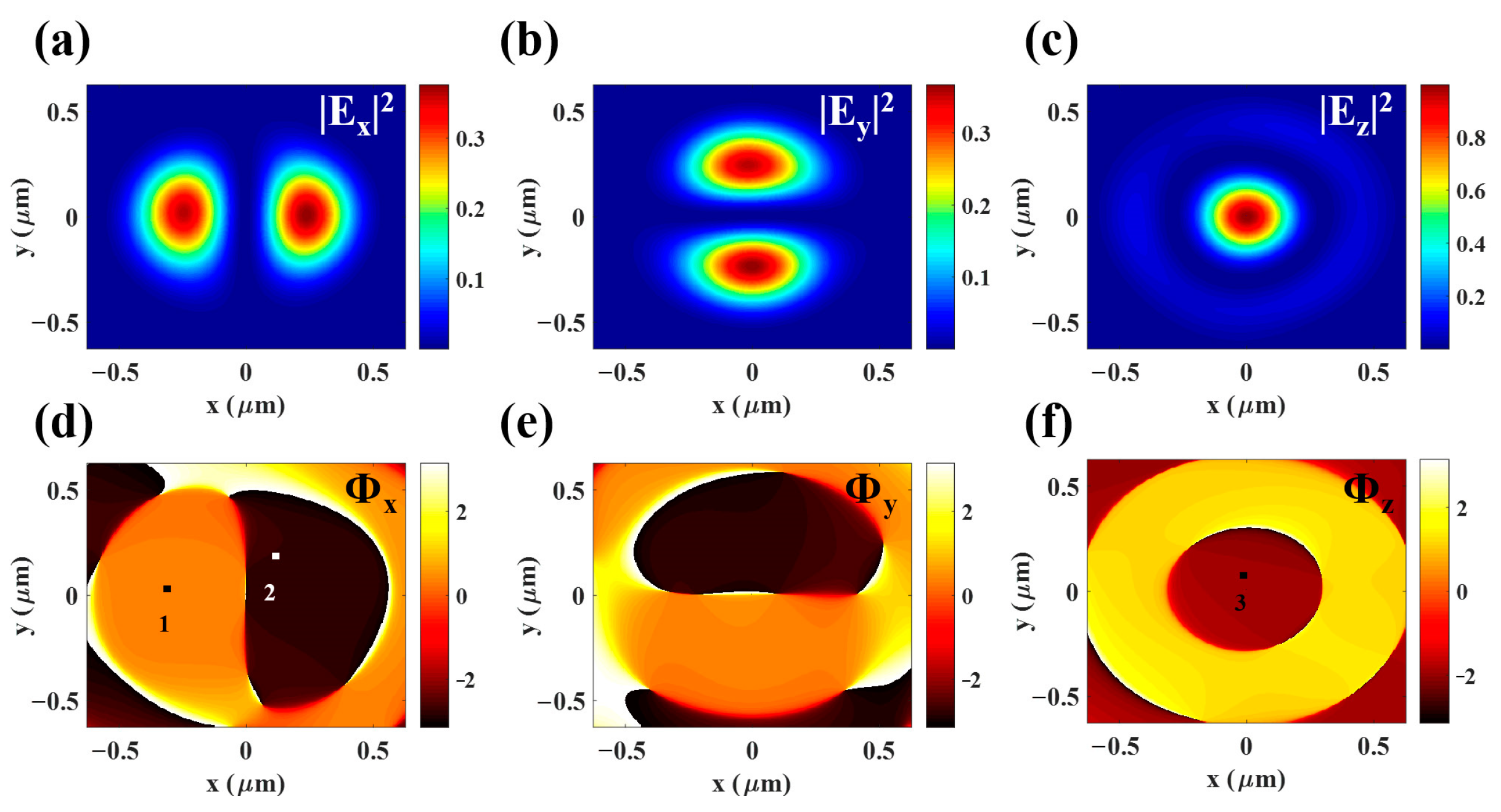
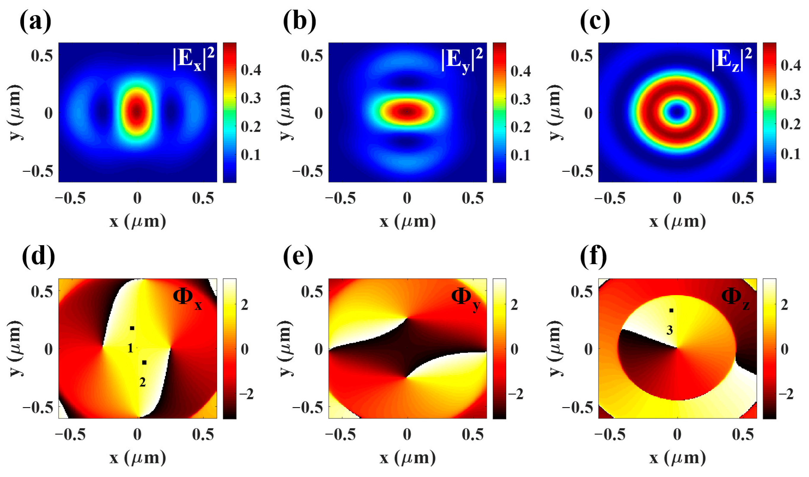
By solving the quadratic equation system, the expansion coefficients of umn and vmn can be uniquely determined. In this work, the maximum n-order of VSHs, including in the reconstruction process, was nmax = 5. By recombining VSHs using these coefficients, the total field in Figure 4 can be obtained. In comparison with the results calculated by Richards–Wolf formulation in Figure 2, the amplitude distribution remains consistent, while the phase distribution shows minor alterations due to the introduction of noise. According to the phase at the three reference points, the results of ϕ1 − ϕ2 = 0.990π, ϕ1 − ϕ3 = 0.493π, and ϕ2 − ϕ3 = −0.497π are basically the same as the theoretical values. Therefore, the proposed method is reasonably robust to noise. To test the convergence of the method with different values of nmax, we conducted a reconstruction of the light field with nmax = 6, the results of which were largely in agreement with those depicted in Figure 4, thus indicating that nmax = 5 is adequate for reconstructing the specific light field.
To further verify the method, the tightly focused field of radially polarized light in Equation (23) with nonzero topological charge was considered. When m0 = 1, using the Richards–Wolf diffraction integral theory, the field distribution expression near the focus is expressed as:
E ( ρ , φ , z ) = k f e i k f 0 θ max g θ e i φ 1 2 i J 0 ( k ρ sin θ ) J 2 ( k ρ sin θ ) cos θ n ^ ρ 1 2 J 0 ( k ρ sin θ ) + J 2 ( k ρ sin θ ) cos θ n ^ φ J 1 ( k ρ sin θ ) sin θ n ^ z e i k z cos θ sin θ d θ .
For the case of m0 = 1, the distributions of the three electric field components in the focal plane (z = 0) is calculated as shown in Figure 5. The reference points for comparison of phase distribution have been marked in Figure 5d–f. The phase difference between each two points can facilitate the validation of the reconstruction results.
The Mie scattering process using a golden nanosphere was analyzed using the proposed numerical model. The power integrations of P x s u m and P y s u m at each scan position are shown in Figure 6. During the scan process, the scan range, scan step, and selected integration regions are consistent with the case of m0 = 0 in Figure 3.
The reconstruction of amplitude and phase distributions are shown in Figure 7. Different from the case of m0 = 0, the Ez-component exhibits a doughnut shape with zero intensity at the center of the beam, where the intensities of transverse components Ex and Ey are enhanced. These features have been comprehensively discussed in previous works [37]. By comparing the results in Figure 5 and Figure 7, the reconstructed field is shown to be consistent with the rigorous calculation results using vector diffraction theory. Therefore, this method is suitable to measure tightly focused fields by various kinds of beams as discussed in Ref. [1].

4. Conclusions

In conclusion, we have theoretically proposed a polarization decomposition method to measure a tightly focused field based on Mie scattering nanointerferometry. By collecting the x- and y-components of the transmitted field from the nanosphere in the far-field region, more constraint equations for the measured expansion coefficients can be obtained. Therefore, the number of spatial scan points and integration regions necessary to solve the inverse scattering problem is reduced, thus making the measurement more efficient. The scheme can acquire the information of scattering field efficiently and provide an excellent platform to study the interaction between light and Mie particles [38].

Author Contributions

Conceptualization, H.H. and Q.Z.; methodology, H.H.; software, D.Y. and H.G; validation, D.Y., H.H. and J.C.; formal analysis, H.G.; investigation, D.Y.; resources, Q.Z.; data curation, H.G.; writing—original draft preparation, D.Y.; writing—review and editing, H.H. and J.C.; visualization, J.C.; supervision, Q.Z.; project administration, H.H.; funding acquisition, H.H. All authors have read and agreed to the published version of the manuscript.

Funding

Our work was supported by the National Natural Science Foundation of China (Projects No. 62075132, No. 92050202, and No. 12274299) and by the Natural Science Foundation of Shanghai (Grant No. 22ZR1443100).

Institutional Review Board Statement

Not applicable.

Informed Consent Statement

Not applicable.

Data Availability Statement

The data presented in this study are available on request from the corresponding author.

Conflicts of Interest

The authors declare no conflict of interest.

Appendix A

In order to ascertain the relationship between the transmission power P and the expansion coefficient, we employed the following derivation process. The intensity pattern of the transmitted light in the far-field region is generated by three terms in Equations (A1)–(A3): the incident power density, the scattering power density from the nanosphere, and the interference term between the two fields.
P in = 1 2 Re E in * × H in ,
P sca = 1 2 Re E sca * × H sca ,
P ext = 1 2 Re E in * × H sca + E sca * × H in .
The interference term in Equation (A3) is defined as the extinction term because it has the same expression with the extinction power in classical Mie theory [28]. This term is essential for retrieving the phase of the incident field, as the phase relationship between the scattering field and the incident field is retained in this term. According to the far-field angular spectra of the vector spherical harmonic functions, the magnetic field components can be calculated using the expansion coefficients of umn and vmn. In this work, the incident field and the scattering field are decomposed into the x-direction and y-direction:
E i n = E i n x x ^ + E i n y y ^ ,
E s c a = E s c a x x ^ + E s c a y y ^ .
where each item in (A4) and (A5) are given in Equations (A6)–(A9):
E i n x = n = 1 + m = n n i n 1 γ m n 4 π u m n m π n m + v m n τ n m cos ϕ i u m m τ n m + v m n m π n m sin ϕ exp i k · r e i m ϕ ,
E i n y = n = 1 + m = n n i n 1 γ m n 4 π u m n m π n m + v m n τ n m sin ϕ + i u m m τ n m + v m n m π n m cos ϕ exp i k · r e i m ϕ ,
E s c a x = n = 1 + m = n n i n 1 γ m n 2 π a m n m π n m + b m n τ n m cos ϕ i a m n τ n m + b m n m π n m sin ϕ exp i k · r e i m ϕ ,
E s c a y = n = 1 + m = n n i n 1 γ m n 2 π a m n m π n m + b m n τ n m sin ϕ + i a m n τ n m + b m n m π n m cos ϕ exp i k · r e i m ϕ .
By combining Equations (A1)–(A9), the power expression for each part can be expressed in matrix form:
P i n ( x / y ) = 1 2 Re u * v * w i n , 11 ( x / y ) w i n , 12 ( x / y ) w i n , 21 ( x / y ) w i n , 22 ( x / y ) u v ,
P s c a ( x / y ) = 1 2 Re a * b * w s c a , 11 ( x / y ) w s c a , 12 ( x / y ) w s c a , 21 ( x / y ) w s c a , 22 ( x / y ) a b ,
P e x t ( x / y ) = 1 2 Re u * v * w e x t , 11 ( x / y ) w e x t , 12 ( x / y ) w e x t , 21 ( x / y ) ) w e x t , 22 ( x / y ) a b + a * b * w e x t , 11 ( x / y ) w e x t , 12 ( x / y ) w e x t , 21 ( x / y ) ) w e x t , 22 ( x / y ) u v .
The total intensities of the transmitted field for x- and y-polarized components in Equation (13) are the sum of Equations (A10)–(A12).

References

  1. Kuznetsov, A.I.; Miroshnichenko, A.E.; Brongersma, M.L.; Kivshar, Y.S.; Luk’yanchuk, B. Optically resonant dielectric nanostructures. Science 2016, 354, 6. [Google Scholar] [CrossRef]
  2. Xu, Y.Z.; Xu, R.H.; Wang, Z.; Zhou, Y.; Shen, Q.F.; Ji, W.C.; Dang, D.F.; Meng, L.J.; Tang, B. Recent advances in luminescent materials for super-resolution imaging via stimulated emission depletion nanoscopy. Chem. Soc. Rev. 2021, 50, 667–690. [Google Scholar] [CrossRef] [PubMed]
  3. Han, X.J.; Xu, K.; Taratula, O.; Farsad, K. Applications of nanoparticles in biomedical imaging. Nanoscale 2019, 11, 799–819. [Google Scholar] [CrossRef] [PubMed]
  4. Baranov, D.G.; Verre, R.; Karpinski, P.; Kall, M. Anapole-Enhanced Intrinsic Raman Scattering from Silicon Nanodisks. ACS Photonics 2018, 5, 2730–2736. [Google Scholar] [CrossRef]
  5. Bogdanov, A.A.; Koshelev, K.L.; Kapitanova, P.V.; Rybin, M.V.; Gladyshev, S.A.; Sadrieva, Z.F.; Samusev, K.B.; Kivshar, Y.S.; Limonov, M.F. Bound states in the continuum and Fano resonances in the strong mode coupling regime. Adv. Photonics 2019, 1, 12. [Google Scholar] [CrossRef]
  6. Rybin, M.V.; Koshelev, K.L.; Sadrieva, Z.F.; Samusev, K.B.; Bogdanov, A.A.; Limonov, M.F.; Kivshar, Y.S. High-Q Supercavity Modes in Subwavelength Dielectric Resonators. Phys. Rev. Lett. 2017, 119, 5. [Google Scholar] [CrossRef]
  7. Hu, H.F.; Gan, Q.Q.; Zhan, Q.W. Achieving maximum scattering circular dichroism through the excitation of anapole states within chiral Mie nanospheres. Phys. Rev. B 2022, 105, 10. [Google Scholar] [CrossRef]
  8. Miroshnichenko, A.E.; Evlyukhin, A.B.; Yu, Y.F.; Bakker, R.M.; Chipouline, A.; Kuznetsov, A.I.; Luk’yanchuk, B.; Chichkov, B.N.; Kivshar, Y.S. Nonradiating anapole modes in dielectric nanoparticles. Nat. Commun. 2015, 6, 8. [Google Scholar] [CrossRef]
  9. Yadav, S.; Devi, A.; De, A.K. Synergistic effect of Fano resonance and optical nonlinearity in laser trapping of silver nanoparticles. Phys. Rev. A 2020, 102, 7. [Google Scholar] [CrossRef]
  10. Koshelev, K.; Kruk, S.; Melik-Gaykazyan, E.; Choi, J.H.; Bogdanov, A.; Park, H.G.; Kivshar, Y. Subwavelength dielectric resonators for nonlinear nanophotonics. Science 2020, 367, 288–292. [Google Scholar] [CrossRef]
  11. Booth, M.J.; Schwertner, M.; Wilson, T.; Nakano, M.; Kawata, Y.; Nakabayashi, M.; Miyata, S. Predictive aberration correction for multilayer optical data storage. Appl. Phys. Lett. 2006, 88, 3. [Google Scholar] [CrossRef]
  12. Xie, X.S.; Chen, Y.Z.; Yang, K.; Zhou, J.Y. Harnessing the Point-Spread Function for High-Resolution Far-Field Optical Microscopy. Phys. Rev. Lett. 2014, 113, 5. [Google Scholar] [CrossRef] [PubMed]
  13. Meier, M.; Romano, V.; Feurer, T. Material processing with pulsed radially and azimuthally polarized laser radiation. Appl. Phys. A-Mater. Sci. Process. 2007, 86, 329–334. [Google Scholar] [CrossRef]
  14. Shvedov, V.; Davoyan, A.R.; Hnatovsky, C.; Engheta, N.; Krolikowski, W. A long-range polarization-controlled optical tractor beam. Nat. Photonics 2014, 8, 846–850. [Google Scholar] [CrossRef]
  15. Quabis, S.; Dorn, R.; Eberler, M.; Glockl, O.; Leuchs, G. The focus of light–theoretical calculation and experimental tomographic reconstruction. Appl. Phys. B-Lasers Opt. 2001, 72, 109–113. [Google Scholar] [CrossRef]
  16. Marchenko, P.; Orlov, S.; Huber, C.; Banzer, P.; Quabis, S.; Peschel, U.; Leuchs, G. Interaction of highly focused vector beams with a metal knife-edge. Opt. Express 2011, 19, 7244–7261. [Google Scholar] [CrossRef]
  17. Schrader, M.; Hofmann, U.G.; Hell, S.W. Ultrathin fluorescent layers for monitoring the axial resolution in confocal and two-photon fluorescence microscopy. J. Microsc.-Oxf. 1998, 191, 135–140. [Google Scholar] [CrossRef]
  18. Nasse, M.J.; Woehl, J.C.; Huant, S. High-resolution mapping of the three-dimensional point spread function in the near-focus region of a confocal microscope. Appl. Phys. Lett. 2007, 90, 3. [Google Scholar] [CrossRef]
  19. Schnell, M.; Garcia-Etxarri, A.; Alkorta, J.; Aizpurua, J.; Hillenbrand, R. Phase-Resolved Mapping of the Near-Field Vector and Polarization State in Nanoscale Antenna Gaps. Nano Lett. 2010, 10, 3524–3528. [Google Scholar] [CrossRef]
  20. Burresi, M.; Engelen, R.; Opheij, A.; van Oosten, D.; Kuipers, L.; Mori, D.; Baba, T. Observation of polarization singularities at the nanoscale. In Proceedings of the 2009 Conference on Lasers and Electro-Optics (CLEO), Baltimore, MD, USA, 2–4 June 2009. [Google Scholar]
  21. Bauer, T.; Orlov, S.; Peschel, U.; Banzer, P.; Leuchs, G. Nanointerferometric amplitude and phase reconstruction of tightly focused vector beams. Nat. Photonics 2014, 8, 24–28. [Google Scholar] [CrossRef]
  22. Bauer, T.; Banzer, P.; Karimi, E.; Orlov, S.; Rubano, A.; Marrucci, L.; Santamato, E.; Boyd, R.W.; Leuchs, G. Observation of optical polarization Mobius strips. Science 2015, 347, 964–966. [Google Scholar] [CrossRef] [PubMed]
  23. Eismann, J.S.; Nicholls, L.H.; Roth, D.J.; Alonso, M.A.; Banzer, P.; Rodriguez-Fortuno, F.J.; Zayats, A.V.; Nori, F.; Bliokh, K.Y. Transverse spinning of unpolarized light. Nat. Photonics 2021, 15, 156–161. [Google Scholar] [CrossRef]
  24. Eismann, J.S.; Banzer, P. Sub-diffraction-limit Fourier-plane laser scanning microscopy. Optica 2022, 9, 455–460. [Google Scholar] [CrossRef]
  25. Li, G.C.; Xiang, J.; Zhang, Y.L.; Deng, F.; Panmai, M.; Zhuang, W.J.; Lan, S.; Lei, D.Y. Mapping the Magnetic Field Intensity of Light with the Nonlinear Optical Emission of a Silicon Nanoparticle. Nano Lett. 2021, 21, 2453–2460. [Google Scholar] [CrossRef] [PubMed]
  26. Takamune, M.; Sasaki, S.; Kondo, D.; Naoi, J.; Kumakura, M.; Ashida, M.; Moriwaki, Y. In situ size measurement of a magnetically trapped single superconducting microparticle by Mie scattering. Appl. Phys. Express 2022, 15, 5. [Google Scholar] [CrossRef]
  27. Hoang, T.X.; Chen, X.D.; Sheppard, C.J.R. Multipole theory for tight focusing of polarized light, including radially polarized and other special cases. J. Opt. Soc. Am. A-Opt. Image Sci. Vis. 2012, 29, 32–43. [Google Scholar] [CrossRef] [PubMed]
  28. Mishchenko, M.I. Scattering, Absorption, and Emission of Light by Small Particles; Cambridge University Press: Cambridge, UK; New York, NY, USA, 2002. [Google Scholar]
  29. Cruzan, O. Translational addition theorems for spherical vector wave functions. Appl. Math. 1962, 20, 33–40. [Google Scholar] [CrossRef]
  30. Zhan, Q.W. Cylindrical vector beams: From mathematical concepts to applications. Adv. Opt. Photonics 2009, 1, 1–57. [Google Scholar] [CrossRef]
  31. Wolf, E.; Sciences, P. Electromagnetic diffraction in optical systems—I. An integral representation of the image field. Proc. R. Soc. Lond. Ser. A Math. Phys. Sci. 1959, 253, 349–357. [Google Scholar]
  32. Richards, B.; Wolf, E.; Sciences, P. Electromagnetic diffraction in optical systems, II. Structure of the image field in an aplanatic system. Proc. R. Soc. Lond. Ser. A Math. Phys. Sci. 1959, 253, 358–379. [Google Scholar]
  33. Dorn, R.; Quabis, S.; Leuchs, G. Sharper focus for a radially polarized light beam. Phys. Rev. Lett. 2003, 91, 4. [Google Scholar] [CrossRef]
  34. Meng, P.W.; Pereira, S.; Urbach, P. Confocal microscopy with a radially polarized focused beam. Opt. Express 2018, 26, 29600–29613. [Google Scholar] [CrossRef]
  35. Zhan, Q.W. Trapping metallic Rayleigh particles with radial polarization. Opt. Express 2004, 12, 3377–3382. [Google Scholar] [CrossRef]
  36. Matsusaka, S.; Kozawa, Y.; Sato, S. Micro-hole drilling by tightly focused vector beams. Opt. Lett. 2018, 43, 1542–1545. [Google Scholar] [CrossRef] [PubMed]
  37. Kozawa, Y.; Sato, S. Focusing of higher-order radially polarized Laguerre-Gaussian beam. J. Opt. Soc. Am. A-Opt. Image Sci. Vis. 2012, 29, 2439–2443. [Google Scholar] [CrossRef] [PubMed]
  38. Foreman, M.R.; Romero, C.M.; Török, P. Determination of the three-dimensional orientation of single molecules. Opt. Lett. 2008, 33, 1020–1022. [Google Scholar] [CrossRef] [PubMed]
Figure 1. (a) The designed setup of the improved Mie scattering nanointerferometry to measure the tightly focused vector field. (b) The schematic of the nanosphere scan process on the focal plane of the upper objective.
Photonics 10 00496 g001
Figure 2. The intensities of the three electric field components, |Ex|2, |Ey|2, |Ez|2, are shown in (a), (b), and (c), respectively. The corresponding phase distributions are shown in (df), with ϕ1 − ϕ2 = π, ϕ1 − ϕ3 = 0.5π, and ϕ2 − ϕ3 = −0.5π.
Photonics 10 00496 g002
Figure 3. Theoretical scanning images of the optical power Px and Py of transmitted light power within different integral regions. The integration regions are adopted with θ 0 , 0.92 and ϕ 0 , 2 π for (a,b), θ 0 , 0.92 and ϕ 0 , 1 for (c,d), and θ 0 , 0.64 and ϕ 0 , 3 for (e,f).
Photonics 10 00496 g003
Figure 4. Reconstruction results of a tightly focused radial polarization vector beam. The intensities of the three electric field components, |Ex|2, |Ey|2, |Ez|2, are shown in (a), (b), and (c), respectively. The corresponding phase distributions are shown in (df), with ϕ1 − ϕ2 = 0.990π, ϕ1 − ϕ3 = 0.493π, and ϕ2 − ϕ3 = −0.497π.
Photonics 10 00496 g004
Figure 5. Theoretical results of a tightly focused vector field for the incident radially polarized beam with m0 = 1. The intensities of the three electric field components, |Ex|2, |Ey|2, |Ez|2, are shown in (a), (b), and (c), respectively. The corresponding phase distributions are shown in (df) with ϕ1 − ϕ2 = 0.018, ϕ1 − ϕ3 = −0.013. and ϕ2 − ϕ3 = −0.310.
Photonics 10 00496 g005
Figure 6. Theoretical scan image of the transmitted light power within specific angular region for RP input beam carrying the topological charge of m0 = 1. The integration regions are θ 0 , 0.92 and ϕ 0 , 2 π for (a,b), θ 0 , 0.92 and ϕ 0 , 1 for (c,d), and θ 0 , 0.64 and ϕ 0 , 3 for (e,f).
Photonics 10 00496 g006
Figure 7. Reconstruction results of a tightly focused vector field for the incident radially polarized beam with m0 = 1. The intensities of the three electric field components, |Ex|2, |Ey|2, |Ez|2, are shown in (a), (b), and (c), respectively. The corresponding phase distributions are shown in (df) with ϕ1 − ϕ2 = 0.004, ϕ1 − ϕ3 = −0.018, and ϕ2 − ϕ3 = −0.220.
Photonics 10 00496 g007
Disclaimer/Publisher’s Note: The statements, opinions and data contained in all publications are solely those of the individual author(s) and contributor(s) and not of MDPI and/or the editor(s). MDPI and/or the editor(s) disclaim responsibility for any injury to people or property resulting from any ideas, methods, instructions or products referred to in the content.

