Communication

Influence of Off-Axis Noncanonical Vortex on the Dynamics of Energy Flux

1
School of Physics and Information Technology, Shaanxi Normal University, Xi’an 710061, China
2
China Academy of Space Technology-Xi’an, Xi’an 710199, China
3
School of Physics, Northwest University, Xi’an 710127, China
4
School of Electronics and Information, Northwestern Polytechnical University, Xi’an 710072, China
*
Authors to whom correspondence should be addressed.
Photonics 2023, 10(3), 346; https://doi.org/10.3390/photonics10030346
Submission received: 27 February 2023 / Revised: 16 March 2023 / Accepted: 17 March 2023 / Published: 22 March 2023
(This article belongs to the Special Issue Coherent and Polarization Optics)

Abstract

:
In this article, we analyze the impact of the off-axis noncanonical vortex on the dynamics of 3D energy flux. The results reveal that the properties of energy flux are significantly influenced by the anisotropy parameter σ c of the off-axis noncanonical vortex. It is demonstrated that by adjusting the anisotropy parameter, we can control the transverse energy flux, from the position of the transverse energy tornado and the distribution of the transverse energy strength to the rotation direction of the transverse energy flux as the beam propagates. The interesting phenomenon, the reversed energy flux, is also closely related to the anisotropy parameter. The position and size of the reversed energy flux region, as well as the production of two energy tornadoes with opposite rotating directions, resembling a Chinese “Taiji” pattern, can be controlled by varying the anisotropy parameter. This result will potentially provide a new freedom for tailoring the 3D optical field and be useful in optical manipulation and processing.

1. Introduction

A traditional vortex beam, which is called a canonical vortex beam, usually indicates intensity zero in its beam center and has a constant phase gradient around the center [1,2], arousing tremendous study on its unique characteristics. Numerous efforts have been devoted to the manipulation of the intensity distribution [3,4], polarization [5,6], coherence [7,8] and energy flux [9,10] of vortex beams and find its wide applications on optical trapping [11], optical tweezers [12] and wireless communications [13]. Additionally, another vortex beam, called the noncanonical vortex beam [14], where the phase gradient and the amplitude were spatially anisotropic, has attracted more attention. The anisotropy parameter “ σ c ” describes the nonlinearity of the phase gradient and exhibits a strong influence on tailoring rich intensity and phase patterns, showing a potential application on the beam shaping [15,16]. Meanwhile, previous research studies concentrate on the properties of the on-axis noncanonical vortex beam, including the intensity, polarization and the energy flow [17,18,19]. In practice, the off-axis vortex is often achieved experimentally [20,21,22,23]. Hence, in this article, we will focus on the off-axis noncanonical vortex beam in a 3D-structured field and its effect on the energy flux.
Besides the intensity and phase, the energy flow is another fundamental quantity offering advantages in its application to 3D optical manipulation. This is where an anomaly phenomenon, energy back propagation, i.e., negative values of the longitudinal Poynting vectors, has attracted researchers. As early as 1919, the backward energy flow near the focus was first revealed by Ignatowskii [24]. Later, Richards and Wolf found the region of the negative propagation light of a strongly focused linearly polarized field in 1959 [25]. From that time and onwards, the condition of the negative energy flow of a sharp focused field with homogeneous (linear, circular and elliptical) polarization [26,27,28] and inhomogeneous (radial and azimuthal) polarization [29,30,31] was studied. Moreover, the negative Poynting vector acting as the “tractor force” on the particle was observed [32]. On the other hand, the transverse energy flow as an informative characteristic of an optical field can usually be decomposed into a spin part and orbit part, inspiring numerous studies on it, such as the spin-to-orbital energy flow conversion [33,34], spin–orbit coupling [35,36], and spin Hall effects of light (SHEL) [37,38]. Here, we will demonstrate that adjusting the anisotropy parameter σ c of the off-axis noncanonical vortex can provide a simple way to control the position of the energy flux tornado, the rotation direction of the energy flux and the region of reversed energy flux, and produce a traditional Chinese “Taiji” pattern. This may be used in many applications, such as when tailoring and enriching the controlled means of particles.

2. Theoretical Background

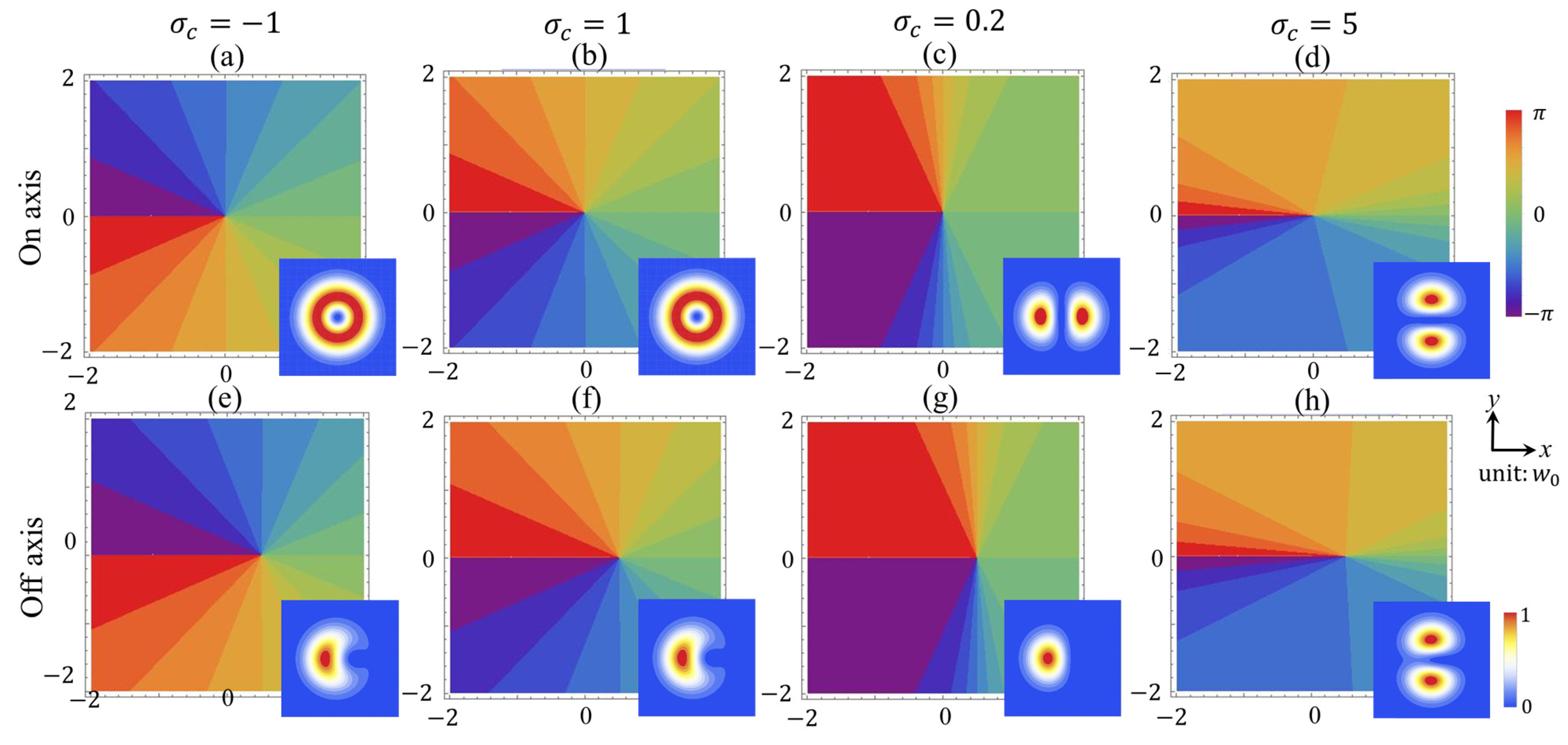
2.1. Noncanonical Vortex

A traditional noncanonical vortex embedded in a beam at location ( a , b ) (in the exit pupil plane of an aplanatic system) can be described as [17]
V in ( x , y ) = A ( x , y ) [ x a + i σ c ( y b ) ] n ,
where A ( x , y ) is the amplitude, and, in this article, the amplitude is assumed to be Gaussian, i.e., A ( x , y ) = e ( x 2 + y 2 ) / w 0 2 with w 0 denoting the waist size of the Gaussian beam. σ c determines the noncanonical strength of the vortex, and as σ c varies, the distributions of both the phase and amplitude change. This is the reason for its name, the anisotropy parameter. In principle, the anisotropy parameter σ c can be a complex number, and when Re [ σ c ] > 0 , the topological charge of the vortex expressed by Equation (1) is n (note n is positive), while for Re [ σ c ] < 0 , the charge is n . In this article, we only focus on the case that σ c is a real number and n = 1 , which means that the vortex is fundamental, and its topological charge is ± 1 . In addition, in order to simplify the discussion, here, we also set b = 0 , i.e., the vortex only can move along the x-axis.
The phase structures of the noncanonical vortex are depicted in Figure 1, where the inserts are their corresponding intensity distributions. In the left two columns, the anisotropy parameter is σ c = ± 1 , and these phase-plots demonstrate that the phase gradient around the vortex is ± 1 . It means that the vortex is actually the canonical type. This also can be found from Equation (1), i.e., when σ c = 1 , the noncanonical vortex degenerates into the canonical vortex. By comparing the phase structures and the intensity distributions for σ c = + 1 and σ c = 1 , we can observe that when σ c changes its sign, only the topological charge is reversed (i.e., the phase gradient changes its sign) but the intensity distribution remains the same. It is easy to demonstrate that this rule is also true for the case | σ c | 1 . Furthermore, from Figure 1, we also can find that for | σ c | < 1 , the phase changes faster near the y-axis, or the (absolute value of) phase gradient becomes bigger near the y-axis; while for | σ c | > 1 , the phase changes faster near the x-axis, or the (absolute value of) phase gradient is bigger there. The effect of the ‘off-axis’ is to push the intensity to the other side of the beam, i.e., to break the symmetry distribution of the intensity.

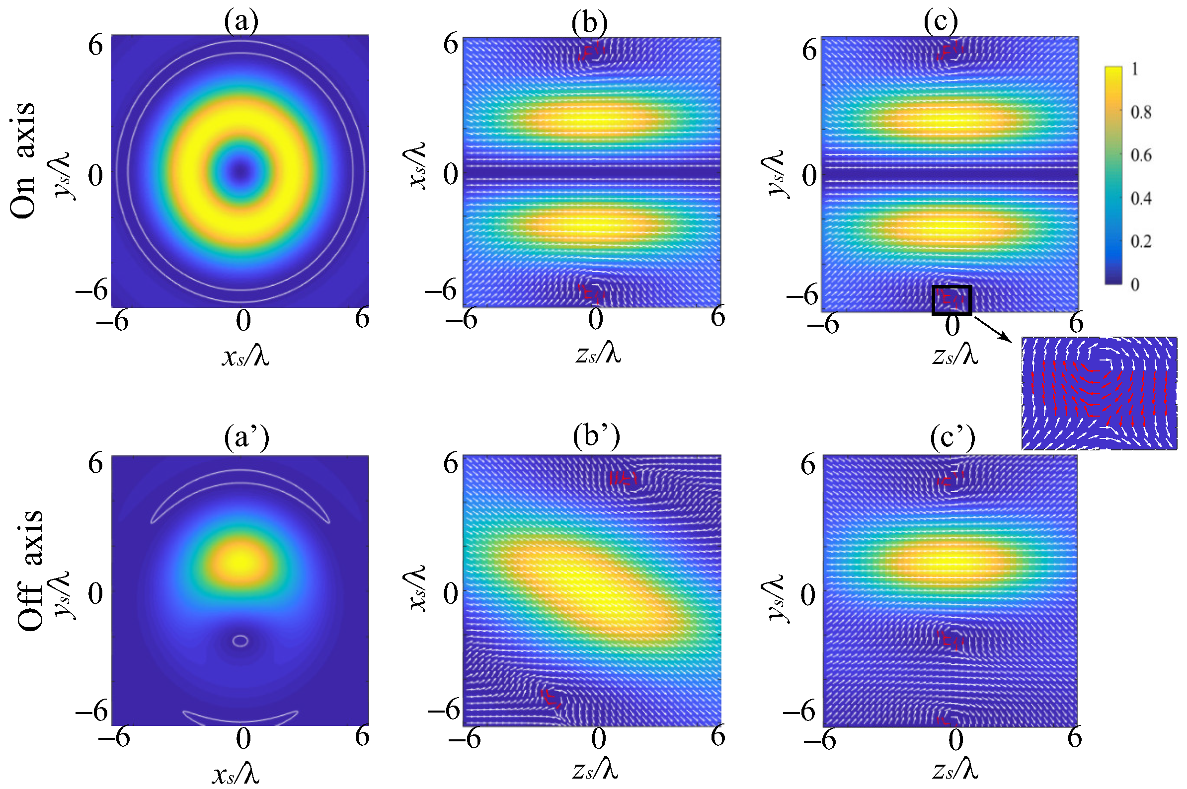
2.2. Electric Field, Magnetic Field and Energy Flux

Here, we will use the noncanonical vortex discussed above to construct a three-dimensional (3D) vector field and derive the expressions of the electric field, magnetic field and energy flux.
Assume that there is an aplanatic, high numerical aperture system with the focal length f and the semi-aperture angle α , and the incident field is an off-axis noncanonical vortex beam described by Equation (1). According to the Richards–Wolf diffraction theory, the electric/magnetic field in the focal region of this structured field at an observation point P ( ρ s , ϕ s , z s ) takes the form:
U ( ρ s , ϕ s , z s ) = i f λ 0 α 0 2 π sin θ cos θ V in ( θ , ϕ ) W p ( θ , ϕ ) e i k z s cos θ × e i k ρ s sin θ cos ( ϕ ϕ s ) d ϕ d θ ,
where U ( ρ s , ϕ s , z s ) represents the electric or magnetic field strength and ( ρ s , ϕ s , z s ) are the cylindrical coordinates. k = 2 π / λ denotes the wave number. Note that here, in order to calculate Equation (2), V in ( x , y ) was changed into V in ( θ , ϕ ) by applying the coordinates transform x = ρ cos ϕ , y = ρ sin ϕ and the Abbe sine condition ρ = f sin θ . The polarization matrix W p ( θ , ϕ ) of the electric or magnetic field in Equation (2) is:
W p ( θ , ϕ ) = 1 + cos 2 ϕ ( cos θ 1 ) sin ϕ cos ϕ ( cos θ 1 ) sin ϕ cos ϕ ( cos θ 1 ) 1 + sin 2 ϕ ( cos θ 1 ) sin θ cos ϕ sin θ sin ϕ w x ( θ , ϕ ) w y ( θ , ϕ )
where w x ( θ , ϕ ) and w y ( θ , ϕ ) are the polarization weight functions of the x component and y component of the incident field. Here, we assume that in this article, the incident field is linearly polarized at a x direction. Thus, for the electric field, the weight functions are w x = 1 and w y = 0 , while for the magnetic field, they are w x = 0 and w y = 1 . By substituting the weight functions into Equation (2), the electric field and the magnetic field in the focal region can be obtained (for more details, one may refer to Appendix A).
For the electric field ( e x , e y , e z ) , after some calculations, their expressions are:
e x ( ρ s , z s , ϕ s ) = i k 0 α P ( θ ) ( I x 0 + I x 1 + I x 2 + I x 3 ) e i k z s cos θ d θ ,
e y ( ρ s , z s , ϕ s ) = i k 0 α P ( θ ) ( I y 1 + I y 2 + I y 3 ) e i k z s cos θ d θ ,
e z ( ρ s , z s , ϕ s ) = i k 0 α P ( θ ) ( I z 0 + I z 1 + I z 2 ) e i k z s cos θ d θ ,
where
P ( θ ) = f e f 2 sin 2 θ / w 0 2 cos θ sin θ ,
and
I x 0 ( θ ; ρ s , ϕ s ) = 1 2 a ( 1 + cos θ ) J 0 ( k ρ s sin θ ) ,
I x 1 ( θ ; ρ s , ϕ s ) = 1 4 f sin θ σ c ( 3 + cos θ ) sin ϕ s + i ( 3 cos θ + 1 ) cos ϕ s J 1 ( k ρ s sin θ ) ,
I x 2 ( θ ; ρ s , ϕ s ) = 1 2 a ( cos θ 1 ) cos 2 ϕ s J 2 ( k ρ s sin θ ) ,
I x 3 ( θ ; ρ s , ϕ s ) = 1 4 f sin θ σ c ( cos θ 1 ) sin 3 ϕ s i ( cos θ 1 ) cos 3 ϕ s J 3 ( k ρ s sin θ ) ,
I y 1 ( θ ; ρ s , ϕ s ) = 1 4 f sin θ σ c ( 1 cos θ ) cos ϕ s i ( 1 cos θ ) sin ϕ s J 1 ( k ρ s sin θ ) ,
I y 2 ( θ ; ρ s , ϕ s ) = 1 2 a ( cos θ 1 ) sin 2 ϕ s J 2 ( k ρ s sin θ ) ,
I y 3 ( θ ; ρ s , ϕ s ) = 1 4 f sin θ σ c ( 1 cos θ ) cos 3 ϕ s + i ( 1 cos θ ) sin 3 ϕ s J 3 ( k ρ s sin θ ) ,
I z 0 ( θ ; ρ s , ϕ s ) = 1 2 f sin 2 θ J 0 ( k ρ s sin θ ) ,
I z 1 ( θ ; ρ s , ϕ s ) = i a sin θ cos ϕ s J 1 ( k ρ s sin θ ) ,
I z 2 ( θ ; ρ s , ϕ s ) = 1 2 f sin 2 θ cos 2 ϕ s + i σ c sin 2 ϕ s J 2 ( k ρ s sin θ ) .
Similarly, the expressions for the components of magnetic field ( h x , h y , h z ) can be derived as
h x ( ρ s , z s , ϕ s ) = i k 0 α P ( θ ) ( T x 1 + T x 2 + T x 3 ) e i k z s cos θ d θ ,
h y ( ρ s , z s , ϕ s ) = i k 0 α P ( θ ) ( T y 0 + T y 1 + T y 2 + T y 3 ) e i k z s cos θ d θ ,
h z ( ρ s , z s , ϕ s ) = i k 0 α P ( θ ) ( T z 0 + T z 1 + T z 2 ) e i k z s cos θ d θ ,
where
T x 1 ( θ ; ρ s , ϕ s ) = 1 4 f sin θ σ c ( 1 cos θ ) cos ϕ s i ( 1 cos θ ) sin ϕ s J 1 ( k ρ s sin θ ) ,
T x 2 ( θ ; ρ s , ϕ s ) = 1 2 a ( cos θ 1 ) sin 2 ϕ s J 2 ( k ρ s sin θ ) ,
T x 3 ( θ ; ρ s , ϕ s ) = 1 4 f sin θ σ c ( 1 cos θ ) cos 3 ϕ s + i ( 1 cos θ ) sin 3 ϕ s J 3 ( k ρ s sin θ ) ,
T y 0 ( θ ; ρ s , ϕ s ) = 1 2 a ( 1 + cos θ ) J 0 ( k ρ s sin θ ) ,
T y 1 ( θ ; ρ s , ϕ s ) = 1 4 f sin θ σ c ( 1 + 3 cos θ ) sin ϕ s + i ( cos θ + 3 ) cos ϕ s J 1 ( k ρ s sin θ ) ,
T y 2 ( θ ; ρ s , ϕ s ) = 1 2 a ( 1 cos θ ) cos 2 ϕ s J 2 ( k ρ s sin θ ) ,
T y 3 ( θ ; ρ s , ϕ s ) = 1 4 f sin θ σ c ( 1 cos θ ) sin 3 ϕ s i ( 1 cos θ ) cos 3 ϕ s J 3 ( k ρ s sin θ ) ,
T z 0 ( θ ; ρ s , ϕ s ) = 1 2 i σ c f sin 2 θ J 0 ( k ρ s sin θ ) ,
T z 1 ( θ ; ρ s , ϕ s ) = i a sin θ sin ϕ s J 1 ( k ρ s sin θ ) ,
T z 2 ( θ ; ρ s , ϕ s ) = 1 2 f sin 2 θ sin 2 ϕ s i σ c cos 2 ϕ s J 2 ( k ρ s sin θ ) .
Obviously, both the electric field and the magnetic field in the focal region are strongly influenced by the anisotropy parameter σ c , as well as the off-axis distance a.
The energy flux, by definition, is expressed by the time-averaged Poynting vector S . Since we have derived all the components of the electric field and magnetic field, now the energy flux can be obtained from the following expression:
S = c 8 π Re ( E × H * ) = S x S y S z = e y h z * e z h y * e z h x * e x h x * e x h y * e y h x * ,
where c is the speed of light in the free space. The superscript * denotes the complex conjugate and Re is the real part of a complex number. Thus, the longitudinal energy flux is represented by S z , which is dependent on the transverse components of both the electric field and the magnetic field; meanwhile, the transverse energy flux is ( S x , S y ) , and from here on we use s x y = ( S x , S y ) to represent this transverse vector, which relies on both the transverse and the longitudinal components of the electromagnetic field.

3. Results and Discussions

In this section, we will analyze the energy flux in the focal region. In order to obtain the effects of the off-axis noncanonical vortex on the dynamics of the energy flux, we will first analyze and summarize the behaviors of the energy flux influenced by the canonical vortex in this section.

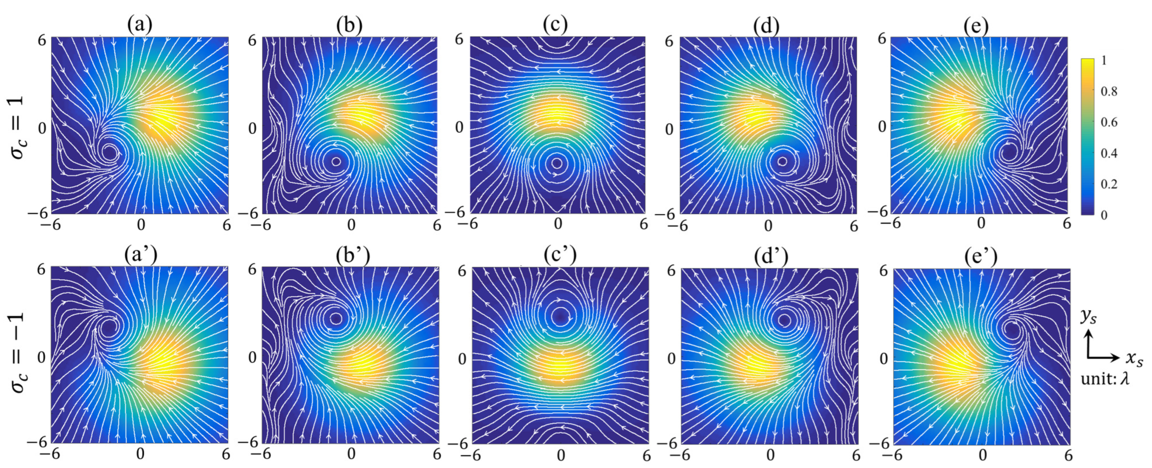
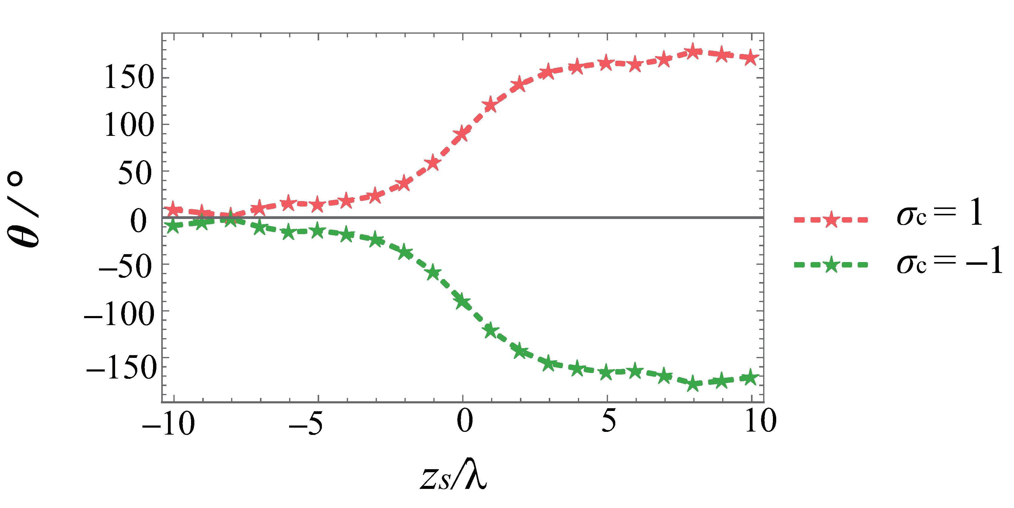
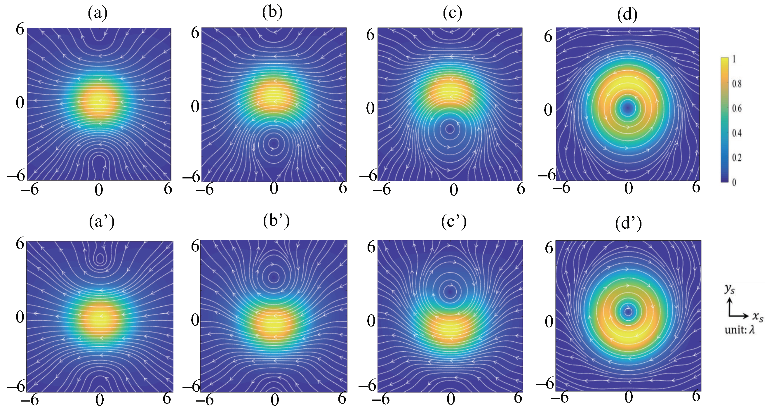
3.1. Energy Flux: The Canonical Vortex Case  | σ c | = 1

For | σ c | = 1 , the incident vortex beam is a canonical type with its topological charge being + 1 (when σ c = + 1 ) or 1 (when σ c = 1 ). Let us first observe the transverse energy flux s x y = ( S x , S y ) in this focused field with | σ c | = 1 . By imputing σ c = ± 1 into Equations (18)–(30), we can obtain the electric field and the magnetic field, and thereby the expression of the transverse energy flux is obtained according to Equation (31).
Figure 2 shows the transverse energy flux s x y including the flow lines (or the lines of the transverse Poynting vectors) and the strength distribution in the focal plane ( z s = 0 ). It can be found, firstly, that there is a (transverse) Poynting singularity, i.e., a transverse energy flux tornado created in the beam center for the off-axis distance a = 0 or along the y s -axis for a 0 . Secondly, the rotation direction of the tornado is counter-clockwise when the anisotropy parameter σ c is positive, whereas it is clockwise when σ c is negative. Thirdly and more interestingly, the sign of σ c determines the location of the energy flux tornado, i.e., the tornado is along the y s -axis if σ c = 1 and along the + y s -axis if σ c = 1 . In other words, the strength maximum of the transverse energy flux or its strength distribution pattern depends on the sign of the anisotropy parameter σ c . This phenomenon is actually caused by both the topological charge of the incident beam and the effect of strongly focusing, which will be discussed in the following.
Propagation of the transverse energy flux s x y in the focal region with z s = 4 λ to z s = + 4 λ is depicted in Figure 3, where the first row shows the case of σ c = + 1 and the second row is the case of σ c = 1 . It can be observe that when σ c > 0 , the energy strength patten (and the energy flux tornado) rotates contour-clockwise as the beam propagates, while for σ c < 0 , it rotates clockwise. In order to illustrate this rotation behavior more clearly, the azimuthal angle of the strength maximum is depicted in Figure 4. (Here, in order to find both the maximum (possible) rotation angle and the tendency of this rotation behavior, the scope which is bigger than the depth of the field, 10 λ z s 10 λ , is chosen.) It is demonstrated that when the beam propagates from z s = 10 λ to 10 λ , the maximum point (representing the strength distribution pattern) of the transverse energy flux rotates from near 0 ( z s = 10 λ ), 90 ( z s = 0 ) to almost 180 ( z s = 10 λ ) for σ c = + 1 and from near 0 ( z s = 10 λ ), 90 ( z s = 0 ) to almost 180 for σ c = 1 . That is to say, that as the beam propagates if σ c > 0 , the strength distribution pattern has a counterclockwise rotation and the total rotation angle is near 180 , while if σ c < 0 , the pattern has a clockwise rotation with the total rotation angle near 180 .
After the discussion on the transverse energy flux, we will examine the longitudinal energy flux. For a common light beam, its longitudinal energy flux usually goes towards the propagation direction, i.e., S z > 0 . The reversed energy flux actually means the longitudinal energy flux S z < 0 , which has special applications in optical trappings. Here, we will observe that in our constructed field, the reserved energy flux can be found.
Figure 5 depicts the strength of the longitudinal energy flow S z on the x O y -plane (in the first column), on the x O z -plane (in the second column) and on the y O z -plane (in the third column), separately. In this figure, the first row shows the on-axis vortex case, i.e., a = 0 , and the second row is the case of a = 0.5 w 0 . In all plots σ c = 1 . The white lines on the x O y -plane denotes S z = 0 and the reverse energy flux exists in the inner region enclosed by the white lines. It is observed that the negative energy flux shows a torus-shape distribution around the beam center for a = 0 , while in the case of a = 0.5 w 0 , the negative energy can distribute near the beam center. In order to illustrate the energy flux with more details, here instead of the flux lines, the energy flux vectors are depicted. The Poynting vectors of s z x = ( S z , S x ) and s z y = ( S z , S y ) denoted by arrows are drawn on the x O z -plane and the y O z plane, respectively. The red ones represent the reversed longitudinal energy flux (the black region with reversed energy flow in Figure 5c is enlarged as an example), i.e., S z < 0 . From Figure 5, it can be found that the off-axis vortex changes the location of the negative energy flux region, while the size of the negative energy flux region is quite modest and almost not influenced by the off-axis vortex.

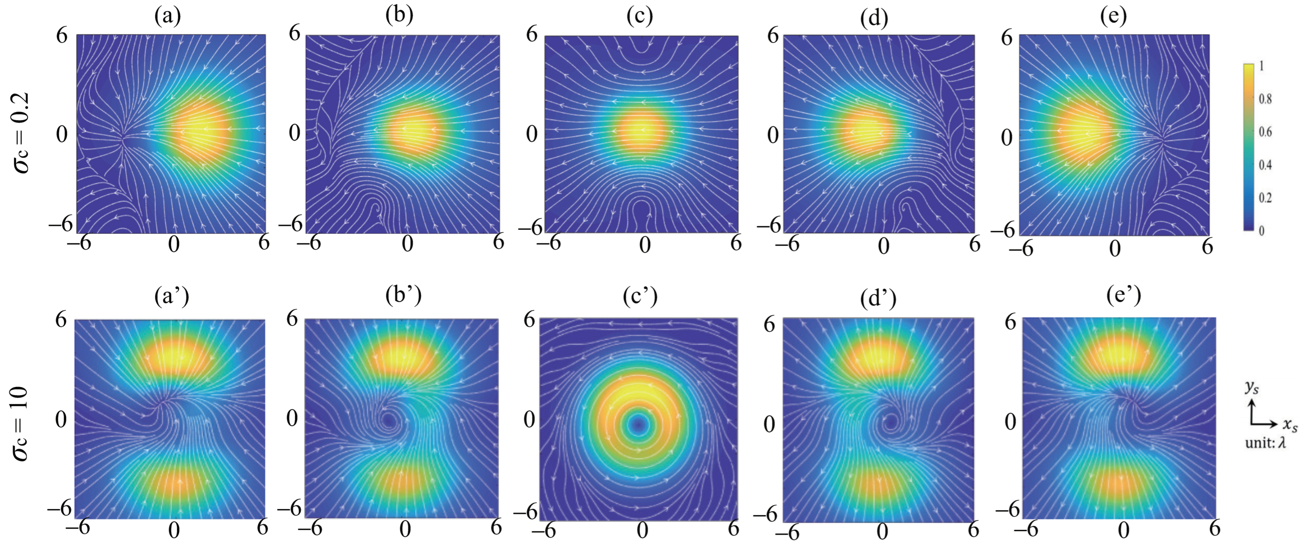
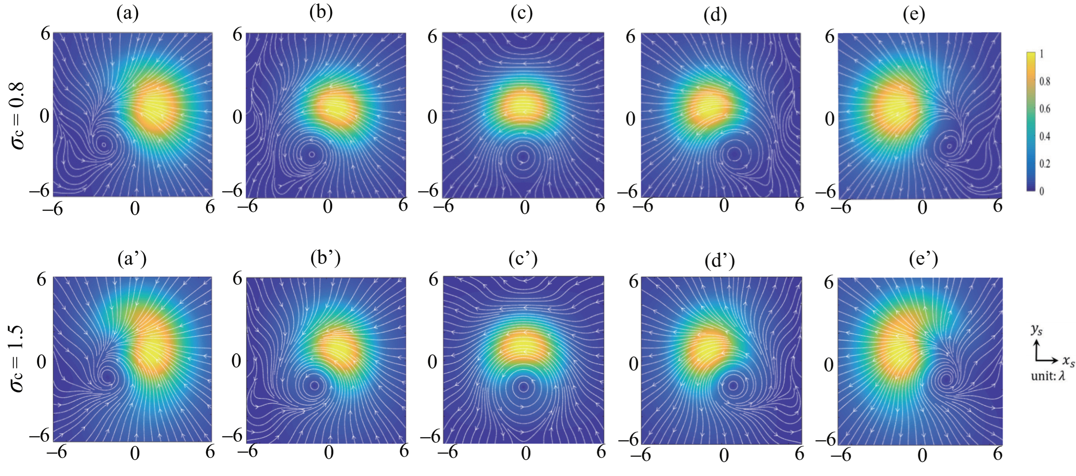
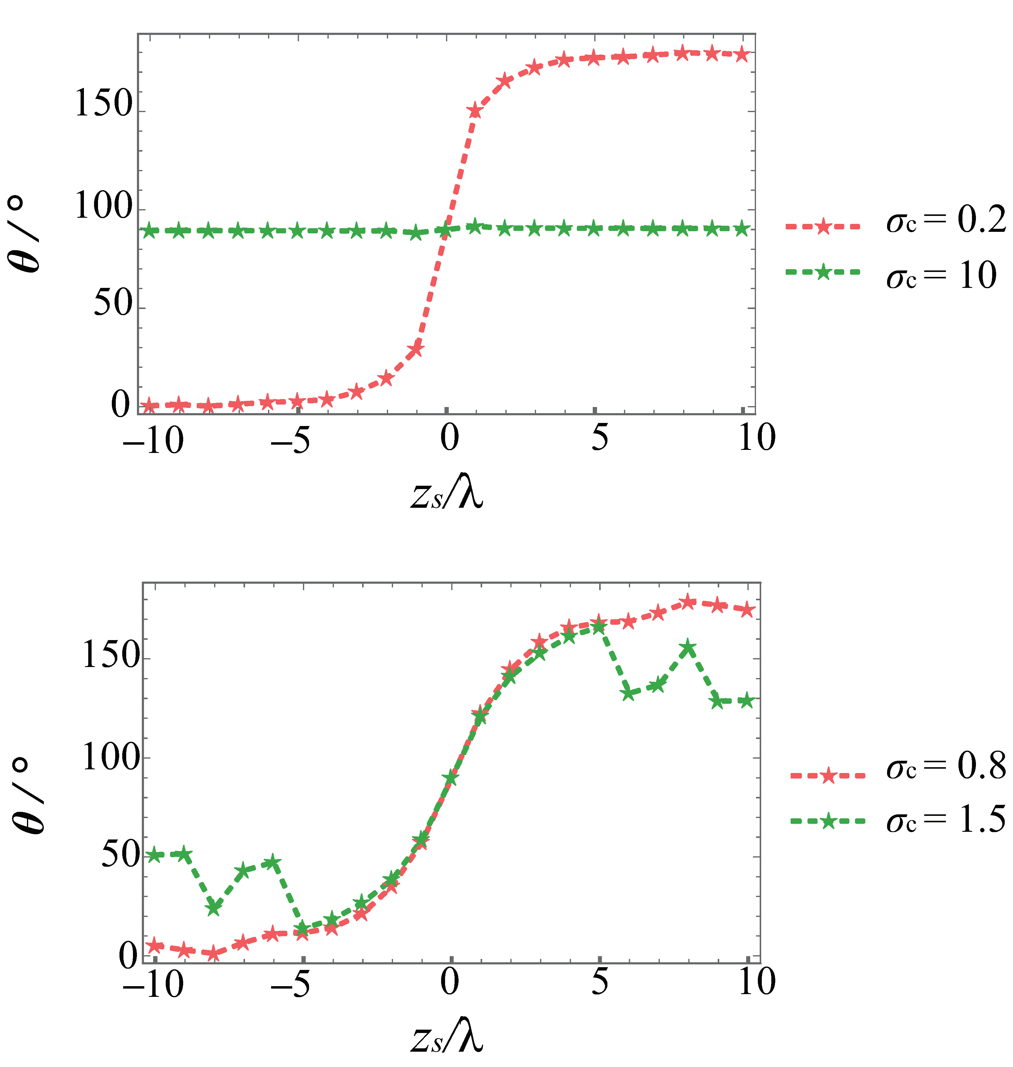
3.2. Energy Flux: The Noncanonical Vortex Case  | σ c | 1

In this part, we will generalize the behaviors of the energy flux influenced by the noncanonical vortex. For | σ c | 1 , the incident vortex beam is the noncanonical type with not only the phase but also the amplitude distributing anisotropically. However, its topological charge remains the same, that is + 1 (when σ c > 0 ) or 1 (when σ c < 0 ).
Similarly, let us first discuss the transverse energy flux in the focused field. The transverse energy flux s x y (including the flow lines and the strength distribution) on the focal plane for different values of the anisotropy parameter σ c is shown in Figure 6. Similar results can be obtained in the case of the noncanonical vortex when compared to the case of the canonical vortex: (a) There is a transverse energy flux tornado (transverse Poynting singularity) along the y s axis for | σ c | 1 with the off-axis vortex a 0 . (b) The rotation direction of the transverse Poynting singularity is counter-clockwise when σ c is positive and clockwise when σ c is negative. (c) The location of the transverse Poynting singularity depends on the sign of σ c . The tornado locates at the y s axis if σ c > 0 and the y s axis if σ c < 0 . Meanwhile, the difference in the results between the canonical and noncanonical cases is that the location of Poynting singularity moves closer to the center as the | σ c | increases. More interestingly, the strength distribution of the transverse energy flux becomes more uniform around the Poynting singularity (near focus) when the | σ c | is much bigger than 1, (see plots (d) and (d’) in Figure 6, σ c = ± 10 ). That is to say, through only adjusting the parameter σ c , we can control the position of the transverse energy tornado and the distribution of the transverse energy strength.
The transverse energy flux s x y for | σ c | 1 along the propagation direction from z s = 4 λ to z s = 4 λ is shown in Figure 7, where the anisotropy parameter σ c = 0.2 in the first row and σ c = 10 in the second row. It is quite obvious that the propagation behavior of the transverse energy flux for | σ c | 1 is very different from that shown in Figure 3 (i.e., | σ c | = 1 ). One can observe that for σ c = 0.2 , 10 , the transverse energy flux s x y seems to not rotate when the beam propagates. The energy strength pattern for σ c = 0.2 has one maximum on the y s -axis on the focal plane, and this maximum laterally moves from the right side (near x s axis) to the left side (near x s axis) as z s increases. When σ c = 10 , the maximum of the energy strength pattern locates at the y s -axis on the focal plane as well, while as the beam propagates, the strength pattern splits into two parts and the maximum moves along the y s -axis. This phenomenon can be physically explained by the joint effect of the anisotropic phase and intensity distribution, as well as the polarization of the incident beam and the strongly focusing. This joint effect results in the energy accumulated along the x s -axis or y s -axis when | σ c | is greatly larger or smaller than 1.
Now, we examine some situations with | σ c | near 1. Figure 8 depicts the transverse energy flux s x y with σ c = 0.8 and 1.5 as the beam propagates. It can be observed that the rotation behavior of s x y is very obvious, which is more like the case for the canonical vortex (see Figure 3). The variations of the azimuthal angles of the strength maximum with the propagation distance for these four cases are shown in Figure 9. From this figure, the rotational behavior and its counterclockwise manner of the transverse energy flux when σ c > 0 can be observed as being more straight.
One can find that the maximum point of the transverse energy flux stays close to 90 , as the beam propagates from z s = 10 λ to z s = 10 λ in the case of σ c = 10 . Meanwhile, for the case of σ c = 0.2 , it is demonstrated that the maximum point of the transverse energy strength stays near 0 when the beam propagates from z s = 10 λ to z s = 3 λ and keeps near 180 when the beam propagates from z s = 3 λ to z s = 10 λ . Note that despite the azimuthal angle of the maximum point not being close to 0 or 180 in the focal region ( z s from 2 λ to 2 λ ), it still changes dramatically from 14 ( z s = 2 λ ) to 166 ( z s = 2 λ ) compared to the canonical vortex case. Moreover, the rotation angle and behavior of the case σ c = 0.8 and 1.5 in Figure 9 confirms the results in Figure 8. It should be noted that the trends of these two curves are not completely the same. There exist differences between σ c = 0.8 and 1.5 in the region z s = 10 λ to 5 λ and z s = 5 λ to 10 λ . This behavior is generated by the anisotropic distribution of the phase and intensity when | σ c | 1 .
The longitudinal energy flow S z of the canonical vortex case has been investigated in detail in Figure 5. Obviously, the longitudinal energy flow becomes more complicated when | σ c | 1 . The strength of longitudinal energy flow and the reverse energy flux region (denoted by the white lines) of σ c = 0.2 , 0.8 , 10 , 15 at the focal plane are shown in Figure 10. Through observing this figure, we can obtain that: (a) For any value of σ c , the strength S z and negative energy flux region is asymmetry distributed on the focal plane. (b) When | σ c | < 1 , the reverse energy flux region, which is near to the focus, becomes bigger and away from the focus as | σ c | decreases. Meanwhile, when | σ c | > 1 , the reverse energy flux region, which is near to the focus, becomes smaller and close to the focus as | σ c | increases. (c) The whole reverse energy flux region on the focal plane becomes bigger as | σ c | increases.
More details of σ c = 0.2 and 15 are shown in Figure 11. The Poynting vectors of s z x and s z y on the x O z -plane and y O z -plane, respectively, are presented by arrows, where the red arrows still denote the reversed longitudinal energy flux. It can be found that not only the location of the negative energy flux region changes with different σ c , but also the size of the negative energy flux region changes as well. Particularly, when σ c = 15 , the negative energy flux region grows in size on the x O z -plane. In order to show energy flux more clearly, we add the energy flow lines of s z x and s z y in Figure 11, which are denoted by white thick lines with arrows. It is very surprising to find that the energy flow lines exhibit an “S” shape and exist two energy flux tornadoes (i.e. Poynting singularities) with opposite topological charges (i.e., opposite rotating directions) on the x O z -plane in the case of σ c = 15 . Even more intriguing is that this “S” shape with two tornadoes is very like the Chinese “Taiji” pattern, where the two tornadoes with opposite charges exactly resemble the two eyes of the “Yin fish” and “Yang fish”, respectively. As the “Yin fish” and “Yang fish” can rotate and be annihilated in the traditional “Taiji” theory, these two energy tornadoes (generated by the reversed energy flux) can also behave in the same way. These two opposite rotating energy tornadoes may provide a simple way to trap and rotate two particles with opposite rotation directions. Moreover, it is obvious that the adjusting anisotropy parameter σ c can manipulate the size and location of the negative longitudinal energy flow region.

4. Conclusions

In this article, an off-axis noncanonical vortex is introduced and its effect on the energy flux of a strongly focused field are discussed. For the transverse energy flux, we find that by adjusting the anisotropy parameter of the nonanonical vortex σ c , we can control the position of the transverse energy tornado and the distribution of the transverse energy strength. Moreover, the rotation direction of the transverse energy flux s x y is determined by the sign of σ c as the beam propagates. There is a special case that when | σ c | is much smaller or bigger than 1, the transverse energy flux s x y seems to not rotate but moves along the x s axis or y s axis, respectively. This phenomenon is physically caused by the joint effect of the anisotropic phase and intensity distribution, the polarization of the incident beam and the strongly focusing. In addition, for the longitudinal energy flux, it is also demonstrated that by changing the anisotropy parameter, σ c can control the location of the reversed energy flux region, the size of the reversed energy flux region and produce two energy tornadoes with opposite rotating directions, resembling a Chinese “Taiji” pattern. Our findings not only examine the fundamental physical properties of an off-axis noncanonical vortex beam, but also provide a theoretical guidance to explore particle control methods in a 3D vector field.

Author Contributions

Conceptualization, X.P.; software, X.Z.; validation, X.Z. and X.P.; formal analysis, X.P. and X.Z.; investigation, X.P. and X.Z.; writing—original draft preparation, X.Z., H.L. and G.W.; writing—review and editing, X.Z and X.P.; visualization, H.L. and G.W. All authors have read and agreed to the published version of the manuscript.

Funding

This research was funded by the National Natural Science Foundation of China (NSFC) (12104283, 11974281, 12074310).

Institutional Review Board Statement

Not applicable.

Informed Consent Statement

Not applicable.

Data Availability Statement

The data presented in this study are available on request from the corresponding author.

Conflicts of Interest

The authors declare no conflict of interest.

Appendix A

Here, we will show some essential steps for obtaining Equations (8)–(30). By substituting the polarization matrix Equation (3) into (2), the electric field in the focal region is obtained:
E ( ρ s , ϕ s , z s ) = e x e y e z = i f λ 0 α 0 2 π sin θ cos θ V in ( θ , ϕ ) 1 + cos 2 ϕ ( cos θ 1 ) sin ϕ cos ϕ ( cos θ 1 ) sin θ cos ϕ × e i k z s cos θ e i k ρ s sin θ cos ( ϕ ϕ s ) d ϕ d θ ,
Similarly, the magnetic field in the focal region is derived as:
H ( ρ s , ϕ s , z s ) = h x h y h z = i f λ 0 α 0 2 π sin θ cos θ V in ( θ , ϕ ) sin ϕ cos ϕ ( cos θ 1 ) 1 + sin 2 ϕ ( cos θ 1 ) sin θ sin ϕ × e i k z s cos θ e i k ρ s sin θ cos ( ϕ ϕ s ) d ϕ d θ ,
where the incident field V in ( θ , ϕ ) in this article is written as follows:
V in ( θ , ϕ ) = e f 2 sin 2 θ / w 0 2 [ f sin θ cos ϕ + i σ c f sin θ sin ϕ a ] .
Taking the x component of the electric field as an example, the key step for deriving the expression of e x is to calculate the integral with respect to ϕ , i.e.,
0 2 π ( f sin θ cos ϕ + i σ c f sin θ sin ϕ a ) ( 1 + cos 2 ϕ ( cos θ 1 ) ) e i k ρ s sin θ cos ( ϕ ϕ s ) d ϕ = 0 2 π 1 4 f sin θ i σ c ( 3 + cos θ ) sin ϕ + ( 3 cos θ + 1 ) cos ϕ + 1 4 f sin θ i σ c ( cos θ 1 ) sin 3 ϕ + ( cos θ 1 ) cos 3 ϕ 1 2 a ( 1 + cos θ ) 1 2 a ( cos θ 1 ) cos 2 ϕ e i k ρ s sin θ cos ( ϕ ϕ s ) d ϕ .
Then by applying the following identities:
0 2 π cos n ϕ e i k ρ s sin θ cos ( ϕ ϕ s ) d ϕ = 2 π i n cos n ϕ s J n ( k ρ s sin θ ) ,
and
0 2 π sin n ϕ e i k ρ s sin θ cos ( ϕ ϕ s ) d ϕ = 2 π i n sin n ϕ s J n ( k ρ s sin θ ) ,
with J n being the first kind Bessel function of order n, Equations (8)–(11) can be obtained. The other components of the electric field and magnetic field can be derived in the same way. Note that the electric and the magnetic field in the focal region in Equations (18)–(20) are consistent with the electric and magnetic field in Ref. [25] when σ c = 1 and a = 0 (except the vortex factor). In addition, the electric field in Equations (8)–(11) in this article and in Ref. [39] are identical for σ c = 1 .

References

  1. Soskin, M.S.; Vasnetsov, M.V. Singular Optics. In Progress in Optics; Wolf, E., Ed.; Elsevier: Amsterdam, The Netherlands, 2001; Volume 42, pp. 219–276. [Google Scholar] [CrossRef]
  2. Gbur, G.J. Singular Optics; Chemical Rubber Company: Boca Raton, FL, USA, 2017. [Google Scholar] [CrossRef]
  3. Otte, E.; Tekce, K.; Denz, C. Tailored intensity landscapes by tight focusing of singular vector beams. Opt. Express 2017, 25, 20194–20201. [Google Scholar] [CrossRef]
  4. Zhao, X.; Pang, X.; Zhang, J.; Wan, G. Transverse Focal Shift in Vortex Beams. IEEE Photon. J. 2018, 10, 1–17. [Google Scholar] [CrossRef]
  5. Kotlyar, V.V.; Kovalev, A.A.; Stafeev, S.S.; Nalimov, A.G.; Rasouli, S. Tightly focusing vector beams containing V-point polarization singularities. Opt. Laser. Technol. 2022, 145, 107479. [Google Scholar] [CrossRef]
  6. Kotlyar, V.V.; Stafeev, S.S.; Nalimov, A.G. Sharp Focusing of a Hybrid Vector Beam with a Polarization Singularity. Photonics 2021, 8, 227. [Google Scholar] [CrossRef]
  7. Dong, M.; Zhao, C.; Cai, Y.; Yang, Y. Partially coherent vortex beams: Fundamentals and applications. Sci. China Phys. Mech. 2021, 64, 224201. [Google Scholar] [CrossRef]
  8. Chen, J.; Liu, X.; Yu, J.; Cai, Y. Simultaneous determination of the sign and the magnitude of the topological charge of a partially coherent vortex beam. Appl. Phys. B-Lasers O 2016, 122, 201. [Google Scholar] [CrossRef]
  9. Angelsky, O.V.; Bekshaev, A.Y.; Maksimyak, P.P.; Maksimyak, A.P.; Hanson, S.G.; Zenkova, C.Y. Orbital rotation without orbital angular momentum: Mechanical action of the spin part of the internal energy flow in light beams. Opt. Express 2012, 20, 3563–3571. [Google Scholar] [CrossRef] [Green Version]
  10. Angelsky, O.V.; Bekshaev, A.Y.; Maksimyak, P.P.; Maksimyak, A.P.; Zenkova, C.Y.; Gorodynska, N.V. Circular motion of particles by the help of the spin part of the internal energy flow. In Proceedings of the ROMOPTO 2012: Tenth Conference on Optics: Micro- to Nanophotonics III, Bucharest, Romania, 3–6 September 2012; Vlad, V.I., Ed.; International Society for Optics and Photonics, SPIE: Bucharest, Romania, 2013; Volume 8882, p. 88820A. [Google Scholar] [CrossRef]
  11. Taylor, M.A.; Waleed, M.; Stilgoe, A.B.; Rubinsztein-Dunlop, H.; Bowen, W.P. Enhanced optical trapping via structured scattering. Nature Photon. 2015, 9, 669–673. [Google Scholar] [CrossRef]
  12. Padgett, M.J.; Molloy, J.; McGloin, D. Optical Tweezers: Methods and Applications; CRC Press: Boca Raton, FL, USA, 2010. [Google Scholar] [CrossRef]
  13. Bozinovic, N.; Yue, Y.; Ren, Y.; Tur, M.; Kristensen, P.; Huang, H.; Willner, A.E.; Ramachandran, S. Terabit-scale orbital angular momentum mode division multiplexing in fibers. Science 2013, 340, 1545–1548. [Google Scholar] [CrossRef] [Green Version]
  14. Freund, I.; Shvartsman, N.; Freilikher, V. Optical dislocation networks in highly random media. Opt. Commun. 1993, 101, 247–264. [Google Scholar] [CrossRef]
  15. Tong, R.; Dong, Z.; Chen, Y.; Wang, F.; Cai, Y.; Setälä, T. Fast calculation of tightly focused random electromagnetic beams: Controlling the focal field by spatial coherence. Opt. Express 2020, 28, 9713–9727. [Google Scholar] [CrossRef] [PubMed]
  16. Pang, X.; Xiao, W.; Zhang, H.; Feng, C.; Zhao, X. X-type vortex and its effect on beam shaping. J. Opt. 2021, 23, 125604. [Google Scholar] [CrossRef]
  17. Molina-Terriza, G.; Wright, E.M.; Torner, L. Propagation and control of noncanonical optical vortices. Opt. Lett. 2001, 26, 163–165. [Google Scholar] [CrossRef]
  18. Roux, F.S. Coupling of noncanonical optical vortices. J. Opt. Soc. Am. B 2004, 21, 664–670. [Google Scholar] [CrossRef]
  19. Kim, G.H.; Lee, H.J.; Kim, J.U.; Suk, H. Propagation dynamics of optical vortices with anisotropic phase profiles. J. Opt. Soc. Am. B 2003, 20, 351–359. [Google Scholar] [CrossRef]
  20. Lopez-Mago, D.; Perez-Garcia, B.; Yepiz, A.; Hernandez-Aranda, R.I.; Gutiérrez-Vega, J.C. Dynamics of polarization singularities in composite optical vortices. J. Opt. 2013, 15, 044028. [Google Scholar] [CrossRef] [Green Version]
  21. Gong, L.; Wang, X.; Zhu, Z.; Lai, S.; Feng, H.; Wang, J.; Gu, B. Transversal energy flow of tightly focused off-axis circular polarized vortex beams. Appl. Opt. 2022, 61, 5076–5082. [Google Scholar] [CrossRef] [PubMed]
  22. Zhang, X.; Li, P.; Liu, S.; Wei, B.; Qi, S.; Fan, X.; Wang, S.; Zhang, Y.; Zhao, J. Autofocusing of ring Airy beams embedded with off-axial vortex singularities. Opt. Express 2020, 28, 7953–7960. [Google Scholar] [CrossRef] [PubMed]
  23. Lee, D.H.; Kim, H.S.; Han, I.; Bae, J.Y.; Yeo, W.J.; Jeong, S.K.; Jeon, M.; Choi, H.J.; Kim, D.U.; Lee, K.S.; et al. Generation of wavelength-tunable optical vortices using an off-axis spiral phase mirror. Opt. Lett. 2021, 46, 4216–4219. [Google Scholar] [CrossRef]
  24. Ignatowsky, V.S. Diffraction by a lens of arbitrary aperture. Trans. Opt. Inst. 1919, 1, 1–36. [Google Scholar]
  25. Richards, B.; Wolf, E. Electromagnetic Diffraction in Optical Systems. II. Structure of the Image Field in an Aplanatic System. Proc. R. Soc. Lond. A 1959, 253, 358–379. [Google Scholar] [CrossRef]
  26. Monteiro, P.B.; Neto, P.A.M.; Nussenzveig, H.M. Angular momentum of focused beams: Beyond the paraxial approximation. Phys. Rev. A 2009, 79, 033830. [Google Scholar] [CrossRef] [Green Version]
  27. Novitsky, A.V.; Novitsky, D.V. Negative propagation of vector Bessel beams. J. Opt. Soc. Am. A 2007, 24, 2844–2849. [Google Scholar] [CrossRef] [PubMed]
  28. Kotlyar, V.V.; Kovalev, A.A.; Nalimov, A.G. Energy density and energy flux in the focus of an optical vortex: Reverse flux of light energy. Opt. Lett. 2018, 43, 2921–2924. [Google Scholar] [CrossRef]
  29. Youngworth, K.S.; Brown, T.G. Focusing of high numerical aperture cylindrical-vector beams. Opt. Express 2000, 7, 77–87. [Google Scholar] [CrossRef]
  30. Zhan, Q.; Leger, J.R. Focus shaping using cylindrical vector beams. Opt. Express 2002, 10, 324–331. [Google Scholar] [CrossRef]
  31. Zhan, Q. Cylindrical vector beams: From mathematical concepts to applications. Adv. Opt. Photon. 2009, 1, 1–57. [Google Scholar] [CrossRef]
  32. Dogariu, A.; Sukhov, S.; Sáenz, J. Optically induced ‘negative forces’. Nat. Photon. 2013, 7, 24–27. [Google Scholar] [CrossRef]
  33. Petersen, J.; Volz, J.; Rauschenbeutel, A. Chiral nanophotonic waveguide interface based on spin-orbit interaction of light. Science 2014, 346, 67–71. [Google Scholar] [CrossRef] [Green Version]
  34. Huang, S.Y.; Zhang, G.L.; Wang, Q.; Wang, M.; Tu, C.; Li, Y.; Wang, H.T. Spin-to-orbital angular momentum conversion via light intensity gradient. Optica 2021, 8, 1231–1236. [Google Scholar] [CrossRef]
  35. Geng, T.; Li, M.; Guo, H. Orbit-induced localized spin angular momentum of vector circular Airy vortex beam in the paraxial regime. Opt. Express 2021, 29, 14069–14077. [Google Scholar] [CrossRef]
  36. Otte, E.; Rosales-Guzmán, C.; Ndagano, B.; Denz, C.; Forbes, A. Entanglement beating in free space through spin–orbit coupling. Light Sci. Appl. 2018, 7, 18009. [Google Scholar] [CrossRef] [PubMed] [Green Version]
  37. Onoda, M.; Murakami, S.; Nagaosa, N. Hall effect of light. Phys. Rev. Lett. 2004, 93, 083901. [Google Scholar] [CrossRef] [PubMed] [Green Version]
  38. Zhu, W.; Zheng, H.; Zhong, Y.; Yu, J.; Chen, Z. Wave-vector-varying Pancharatnam-Berry phase photonic spin Hall effect. Phys. Rev. Lett. 2021, 126, 083901. [Google Scholar] [CrossRef] [PubMed]
  39. Zhao, X.; Zhang, J.; Pang, X.; Wan, G. Properties of a strongly focused Gaussian beam with an off-axis vortex. Opt. Commun. 2017, 389, 275–282. [Google Scholar] [CrossRef]
Figure 1. Structure of noncanonical vortex. The big plots are phase distributions and the inserts are their corresponding intensity distributions. In the first row, the vortex is located at the beam center, and in the second row, it is off-axis with a = 0.5 w 0 . In the left two columns σ c = ± 1 [(a,b,e,f)], i.e., the vortex degenerates into the canonical type.
Photonics 10 00346 g001
Figure 2. The transverse energy flux s x y with flow lines (in white) and strength | s x y | (color-coded) on the focal plane. Here (a) σ c = 1 , a = 0 (b) σ c = 1 , a = 0 , (c) σ c = 1 , a = 0.5 w 0 and (d) σ c = 1 , a = 0.5 w 0 . In all plots: f = 2 mm, w 0 = 2 mm and α = 60 .
Photonics 10 00346 g002
Figure 3. The transverse energy flux s x y along the propagation direction. Here, (a,a’) z s = 4 λ , (b,b’) z s = 2 λ , (c,c’) z s = 0 , (d,d’) z s = 2 λ and (e,e’) z s = 4 λ . In all plots: a = 0.5 w 0 , f = 2 mm, w 0 = 2 mm and α = 60 .
Photonics 10 00346 g003
Figure 4. The rotation angle for the transverse energy flux s x y with the beam propagation. Here, a = 0.5 w 0 , f = 2 mm, w 0 = 2 mm and α = 60 .
Photonics 10 00346 g004
Figure 5. The longitudinal energy flow S z on the (a,a’) x O y -plane, (b,b’) x O z -plane and (c,c’) y O z -plane. In (ac) σ c = 1 , a = 0 , (a’c’) σ c = 1 , a = 0.5 w 0 . In all plots, f = 2 mm, w 0 = 2 mm and α = 60 .
Photonics 10 00346 g005
Figure 6. The transverse energy flux s x y with flow lines and strength | s x y | on the focal plane for | σ c | 1 . Here, (a) σ c = 0.2 , (a’) σ c = 0.2 , (b) σ c = 0.8 , (b’) σ c = 0.8 , (c) σ c = 1.5 , (c’) σ c = 1.5 and (d) σ c = 10 , (d’) σ c = 10 . In all plots, a = 0.5 w 0 , f = 2 mm, w 0 = 2 mm and α = 60 .
Photonics 10 00346 g006
Figure 7. The transverse energy flux s x y along the propagation direction. Here, (a,a’) z s = 4 λ , (b,b’) z s = 2 λ , (c,c’) z s = 0 , (d,d’) z s = 2 λ and (e,e’) z s = 4 λ . In all plots: a = 0.5 w 0 , f = 2 mm, w 0 = 2 mm and α = 60 .
Photonics 10 00346 g007
Figure 8. The transverse energy flux s x y along the propagation direction. Here, (a,a’) z s = 4 λ , (b,b’) z s = 2 λ , (c,c’) z s = 0 , (d,d’) z s = 2 λ and (e,e’) z s = 4 λ . In all plots: a = 0.5 w 0 , f = 2 mm, w 0 = 2 mm and α = 60 .
Photonics 10 00346 g008
Figure 9. The rotation angle for the transverse energy flux s x y with the beam propagation. Here, a = 0.5 w 0 , f = 2 mm, w 0 = 2 mm and α = 60 .
Photonics 10 00346 g009
Figure 10. The longitudinal energy flow S z on the x O y -plane, where (a) σ c = 0.2 , (b) σ c = 0.8 , (c) σ c = 10 and (d) σ c = 15 . In all plots, a = 0.5 w 0 , f = 2 mm, w 0 = 2 mm and α = 60 .
Photonics 10 00346 g010
Figure 11. The longitudinal energy flow S z on the (a,a’) x O y -plane, (b,b’) x O z -plane and (c,c’) y O z -plane. Where (ac) σ c = 0.2 and (a’c’) σ c = 15 . In all plots, a = 0.5 w 0 , f = 2 mm, w 0 = 2 mm and α = 60 .
Photonics 10 00346 g011
Disclaimer/Publisher’s Note: The statements, opinions and data contained in all publications are solely those of the individual author(s) and contributor(s) and not of MDPI and/or the editor(s). MDPI and/or the editor(s) disclaim responsibility for any injury to people or property resulting from any ideas, methods, instructions or products referred to in the content.

