Estimation Method Based on Extended Kalman Filter for Uncertain Phase Shifts in Phase-Measuring Profilometry

Abstract

Phase-measuring profilometry (PMP) is increasingly applied in high-accuracy three-dimensional shape measurement. However, various factors may result in the uncertainty of phase shift values in the PMP system, and phase errors induced by actual phase shift often bring about the reconstruction failure of a measured object. A quadratic phase estimation method using the extended Kalman filter is proposed to remove the phase error introduced by uncertain phase shift. After eliminating the background and fringe modulation, the state estimation is employed to evaluate the quadratic phase coefficients in a selected mask window, and the phase shifts of adjacent fringe patterns can be estimated to compute the unwrapping phase. This paper presents a novel method for improving the accuracy of the PMP system influenced by phase shift errors, and the proposed region-wise method significantly enhances the reconstruction quality and efficiency. Experimental results show that the proposed algorithm effectively evaluates the actual phase shift and directly compensates the phase error, and has the advantages of high speed, high accuracy, and robustness.

1. Introduction

Three-dimensional (3-D) measurements have developed rapidly and have received extensive attention over the past three decades [1]. Fourier transform profilometry (FTP) [2] has the merits of single frame, high speed, on-line, and non-contact measurement, but it is not available for complex objects. Phase-measuring profilometry (PMP) is widely used in 3-D reconstruction due to its advantages of high accuracy, robustness, and insensitivity to the changes of ambient illumination and surface reflectance [3,4,5]. The phase information can be retrieved by the multi-frame phase-shifting fringe patterns of a measured object.

A fixed phase shift is set among the multiple fringe patterns in PMP [6]. However, in real scenarios, any motion of the measured object and mechanical projection device will induce phase shift errors [7,8,9], thereby leading to measurement error. Phase shift errors generated by various factors are ones of uncertainty, with many researchers drawn to address the issue in the PMP system. It is inevitable that the phase shift errors affect the accuracy of the phase reconstruction when exploiting the phase-shifting method [10]. Hyun et al. [11] developed a metal-based pattern generation mechanical device, and generated the phase shift fringe patterns by using the precise synchronization of a camera and a projector to achieve accurate shape restoration. Liu et al. [12] proposed a rotary mechanical projector to carry out shape measurement, with a probability distribution function (PDF) introduced to address the error correction with different phase-shifting error. Although the application of the digital projection devices greatly reduces the phase shift errors generated from a mechanical projector, the PMP system may also have random phase shift error while it is used to measure an object moving at high speed.

Different methods are proposed to address phase shift errors caused by the object motion, such as the object tracking method [13,14], Fourier-assisted PMP method [8,15,16], iterative least-squares method [17,18], average phase method [19], Hilbert transform method [20], statistical nature compensation method [21], deep learning-based reconstruction method [22,23,24], and motion prediction method [25,26], which significantly reduces the error caused by the object’s movement. Guo et al. [13] proposed a Lucas–Kanade optical flow method to estimate the displacement of each pixel by capturing object images in the beginning and ending states. The displacement of each pixel is computed by the markers and the phase map is obtained from a five-step phase-shifting algorithm, which precisely settles the phase jump caused by the object’s motion and ideal phase shift, but it is not available for non-uniform motion. Lu et al. [18] improved the measuring accuracy performance for the in-motion object using the advanced iterative algorithm (AIA) [17], and then presented a method by projecting two fringe patterns with different frequencies to compensate the motion errors for an isolated motion object, with the position mismatches and phase variation between the two frequencies employed to reconstruct the isolated object [14]. Moreover, motion prediction methods have been developed to deal with this issue. Han et al. [25] presented the pixel movement estimation method in the phase-shifting fringe patterns, and identified the corresponding pairs by the features in the object. Liu et al. [26] proposed an estimation method by comparing the difference of the same point between two subsequent 3-D frames, with the phase shift error for each pixel estimated and used to compensate for the phase errors. The main strength of the above two prediction methods is that their methods compensate for motion errors at the pixel-wise, thus resulting in high accuracy.

Our goal is to develop a fast and effective method to eliminate the phase error induced by the imprecise phase shift and enhance the reconstruction accuracy. A three-step phase-shifting algorithm is selected to reconstruct the object shape due to the minimum number of fringe patterns satisfying the accuracy requirements. Fringe patterns using a window within a mask are used to evaluate the phase shift, and the background and fringe modulation are removed from the selected region-wise fringe patterns. A two-dimensional quadratic function is employed to approximate the phase of the measured object within a mask window, with quadratic phase coefficients estimated by exploiting the extended Kalman filter (EKF) method. The actual interframe phase shift estimation can be acquired with the relationship between the phase function coefficients; after demodulating the fringe pattern to obtain the wrapped phase by using the least-squares algorithm, the continuous phase of the object is recovered by the spatial unwrapping method. Experimental results show the high speed, high accuracy, and robustness for uncertain phase shift estimation of the proposed region-wise method in the PMP system.

2. Principle

2.1. The Phase Estimation Model

The intensity distributions of the three-step phase-shifting algorithm can be described as [27]:

$$I_n(x,y)=a(x,y)+b(x,y)\cos [\varphi (x,y)+\frac{2\pi (n-1)}{3}]\begin{array}{cc}& \mathrm{n}=1,2,3\end{array}$$

(1)

where I_n(x,y) denotes the intensity of the recorded patterns, a(x,y) and b(x,y) denote the background intensity and fringe modulation, respectively, and ϕ(x,y) is the object phase. The wrapped phase can be calculated by:

$$\mathrm{\Phi }(x,y)=\arctan [\frac{{\displaystyle {\sum }_{n=1}^N(I_n(x,y)\sin 2\pi (n-1)/N)}}{{\displaystyle {\sum }_{n=1}^N(I_n(x,y)\cos 2\pi (n-1)/N)}}]$$

(2)

The additional unknown phase shift errors caused by factors such as an object’s motion or mechanical projector’s error will result in:

$$I_n(x,y)=a(x,y)+b(x,y)\cos [\varphi (x,y)+\frac{2\pi (n-1)}{3}+{\delta }_{n-1}]$$

(3)

where δ_n−1 denotes the additional phase step errors of two adjacent patterns.

The phase of the captured object is the focus of our attention in the 3-D reconstruction, and the additional phase errors are an important factor to introduce the phase error. An accurate estimation of δ_n−1 will be of benefit to obtain the exact phase. The background intensity and modulation change slowly in the projection of the structured light fringe. The parameters a_n(x,y), b_n(x,y), ϕ(x,y), and δ_n−1 are unknown, while I_n(x,y) is known. In order to reduce the influence of non-uniform background light and noise, a_n(x,y) and b_n(x,y) are removed from the intensity I_n(x,y) to enhance the estimation reliability and reduce the number of unknown parameters. The fringe pattern after removing the background a_n(x,y) using the frequency domain filtering can be expressed as:

$${\tilde{I}}_n(x,y)=b(x,y)\cos [\varphi (x,y)+\frac{2\pi (n-1)}{3}+{\delta }_{n-1}]$$

(4)

After normalizing the captured fringe patterns, Equation (4) can then be rewritten as:

$${\widehat{I}}_n(x,y)=\cos [\varphi (x,y)+{\epsilon }_n]$$

(5)

where ε_n denotes the phase shift relative to ϕ(x,y) of the nth pattern, which contains the fixed phase shift 2π(n − 1)/3 and the additional phase step error δ_n−1.

A 2-D quadratic phase function is employed to approximate the object phase in a 2-D window. To express the quadratic phase function, we set ϕ_n (x, y) = ϕ (x,y) + ε_n. The quadratic phase function ϕ_n (x,y) of the three-step phase-shifting profilometry is defined as:

$$\left\{\begin{array}{l}{\varphi }_1(x,y)={\alpha }_0+{\alpha }_{1}x+{\alpha }_{2}y+{\alpha }_3{x}^2+{\alpha }_{4}xy+{\alpha }_5{y}^2\\ {\varphi }_2(x,y)={\alpha }_6+{\alpha }_{1}x+{\alpha }_{2}y+{\alpha }_3{x}^2+{\alpha }_{4}xy+{\alpha }_5{y}^2\\ {\varphi }_3(x,y)={\alpha }_7+{\alpha }_{1}x+{\alpha }_{2}y+{\alpha }_3{x}^2+{\alpha }_{4}xy+{\alpha }_5{y}^2\end{array}\right.$$

(6)

where α_i is the quadratic phase coefficient. When the surface shape of the object changes gently, all phase regions can be roughly approximated by the quadratic phase approximation. However, when the surface shape of the object changes dramatically, the phase shift errors obtained by the whole phase approximation will increase due to the large difference in the phase of each part of the object. To enhance the estimation accuracy and the computation efficiency, a linear region of the fringe pattern is selected to approximate the quadratic phase and estimate the interframe phase shift. The phase shift is evaluated by processing a small region instead of the full-field pixel-by-pixel estimation, which can improve the computation speed and effectiveness.

A selected window in the selected mask with the linear phase is used for phase shift estimation. The fringe within the window can be expressed as:

$${\widehat{I}}_{nw}(x,y)=\cos [{\varphi }_n(x,y)] (x,y)\in \mathrm{window}$$

(7)

where ϕ_n (x, y), $(x,y)\in \mathrm{window}$ denotes the phase of the selected linear region. It is theoretically well known that ε₁ = 0, ε₂ = 2π/3, and ε₃ = 4π/3 in the three-step phase-shifting method, but ε_n is no longer the fixed phase shift in the case of the mechanical projection and/or moving object, which contains the fixed phase shift and additional phase step errors. It is greatly pivotal to obtain the additional phase step errors for the phase maps retrieval. According to the definition of the quadratic phase, we have ε₂ = α₆ − α₀ and ε₃ = α₇ − α₀. The EKF estimation method is used to estimate the phase coefficients to obtain the actual phase shift caused by various factors.

2.2. Phase Shift Estimation Based on Extended Kalman Filter

The state estimation method is widely used in robotics, speech, automatic control, communication, biomedicine, and image processing [28]. Kalman filter (KF) is an optimal solution for the linear filtering problem, but most practical systems are nonlinear. EKF is considered as an extended form of the KF in the nonlinear case [29,30]. It is an efficient method to solve the nonlinear state estimation problem by using Taylor series expansion, and utilizes the KF framework to process the data, which is a type of suboptimal filtering. EKF gives an approximation of the optimal estimate, and can provide an estimate of the system’s state based on its measurements, but it may diverge if continuous linearization is not a good approximation to the linear model in all the uncertainty domains. The system and observation dynamics of the nonlinearization model are linearized to implement the KF framework around the last state estimate. The process of EKF can be summarized as: prior estimation, prior estimation error update, filter gain update, state optimal estimation, and optimal estimation error update.

The fixed phase shift values become uncertain phase shifts due to various factors in the practical application. If no compensation or improvement is made, phase errors will be caused. The measured object’s phase is approximated as a 2-D quadratic function in a mask window, and the quadratic phase function is a typical nonlinear problem. The EFK method is a robust and promising approach to evaluate the coefficients. The coefficients of the quadratic phase function are taken as elements of the state vector and estimated in this approach, with the actual phase shifts to be obtained from the quadratic function coefficients.

The observation vector of fringe patterns I_obi (i = 1, 2) is defined as:

$$I_{ob1}=\left[\begin{array}{l}{\widehat{I}}_{1w}(x,y)\\ {\widehat{I}}_{2w}(x,y)\end{array}\right], I_{ob2}=\left[\begin{array}{l}{\widehat{I}}_{2w}(x,y)\\ {\widehat{I}}_{3w}(x,y)\end{array}\right] (x,y)\in \mathrm{window}$$

(8)

The state vector λ_i of the three-step phase-shifting algorithm is defined as:

$$\left\{\begin{array}{l}{\mathit{\lambda }}_1={[{\alpha }_0, {\alpha }_1, {\alpha }_2, {\alpha }_3, {\alpha }_4, {\alpha }_5, {\alpha }_6]}^T\\ {\mathit{\lambda }}_2={[{\alpha }_6, {\alpha }_1, {\alpha }_2, {\alpha }_3, {\alpha }_4, {\alpha }_5, {\alpha }_7]}^T\end{array}\right.$$

(9)

The initial estimation state vector ${\widehat{\mathit{\lambda }}}_{i0|0}$ and covariance matrix $P_{i0|0}$ are assumed as:

$${\widehat{\mathit{\lambda }}}_{i0|0}=E({\mathit{\lambda }}_{i0}), P_{i0|0}=E[({\mathit{\lambda }}_{i0}-{\widehat{\mathit{\lambda }}}_{i0|0}){({\mathit{\lambda }}_{i0}-{\widehat{\mathit{\lambda }}}_{i0|0}]}^T$$

(10)

EKF comprises the time update and measurement update. EKF linearizes the system based on prior estimates, and estimates the predicted value of the current time by using the estimated value of the previous time, which is in good agreement with the estimation of the quadratic phase coefficient, and the coefficient estimated values of the previous pixel are utilized to estimate the predicted values at the next pixel. Time update is defined as follows:

$${\widehat{\mathit{\lambda }}}_{ik|k-1}=\mathbf{F}{\widehat{\mathit{\lambda }}}_{ik-1|k-1}$$

(11)

$${\mathbf{P}}_{ik|k-1}=\mathbf{F}{P}_{ik-1|k-1}{\mathbf{F}}^T$$

(12)

where ${\widehat{\mathit{\lambda }}}_{ik|k-1}$ and $P_{ik|k-1}$, respectively, denote the predicted state vector and corresponding predicted error covariance matrix at the kth step derived by the (k − 1)th pixel. F is a 7 × 7 identity matrix. Since F is set to be the identity matrix, the predicted values of the state vector are the coefficient estimates of the previous pixel.

The normalized fringe patterns and their prediction are utilized to estimate the actual phase shifts, with the measurement update formulated by:

$${\mathbf{K}}_{ik}=P_{ik|k-1}{\mathbf{H}}_{ik}^T{({\mathbf{H}}_{ik}{P}_{ik|k-1}{\mathbf{H}}_{ik}^T+{\mathbf{R}}_{ik})}^{-1}$$

(13)

$${\widehat{\mathit{\lambda }}}_{ik|k}={\widehat{\mathit{\lambda }}}_{ik|k-1}+{\mathbf{K}}_k[I_{obi}-h({\widehat{\mathit{\lambda }}}_{ik|k-1})]$$

(14)

$${\mathbf{P}}_{ik|k}=P_{ik|k-1}-{\mathbf{K}}_{ik}{\mathbf{H}}_{ik}{P}_{ik|k-1}$$

(15)

where K_ik and R_ik represents the Kalman gain and observation noise covariance matrix, respectively. The predicted nonlinear observation vector $h({\widehat{\mathit{\lambda }}}_{ik|k-1})$ is calculated by linearization using the first-order partial derivation of Taylor series expansion, which is given by:

$$h({\widehat{\mathit{\lambda }}}_{ik|k-1})={\mathbf{H}}_{ik}\left[\begin{array}{l}\cos ({\widehat{\mathit{\lambda }}}_{ik|k-1}{s}_1)\\ \cos ({\widehat{\mathit{\lambda }}}_{ik|k-1}{s}_2)\end{array}\right]$$

(16)

where H_ik represents the Jacobian matrix of the phase measurement function at ${\widehat{\mathit{\lambda }}}_{ik|k-1}$ given by:

$${\mathbf{H}}_{ik}=-\left[\begin{array}{lllllll}\hfill \sin ({\widehat{\varphi }}_i),\hfill & \hfill \sin ({\widehat{\varphi }}_i)x,\hfill & \hfill \sin ({\widehat{\varphi }}_i)y,\hfill & \hfill \sin ({\widehat{\varphi }}_i)x^2,\hfill & \hfill \sin ({\widehat{\varphi }}_i)xy,\hfill & \hfill \sin ({\widehat{\varphi }}_i)y^2,\hfill & \hfill 0\hfill \\ \hfill 0,\hfill & \hfill \sin ({\widehat{\varphi }}_{i+1})x,\hfill & \hfill \sin ({\widehat{\varphi }}_{i+1})y,\hfill & \hfill \sin ({\widehat{\varphi }}_{i+1})x^2,\hfill & \hfill \sin ({\widehat{\varphi }}_{i+1})xy,\hfill & \hfill \sin ({\widehat{\varphi }}_{i+1})y^2,\hfill & \hfill \sin ({\widehat{\varphi }}_{i+1})\hfill \end{array}\right]\begin{array}{cc}& (i=1,2)\end{array}$$

(17)

where ${\widehat{\varphi }}_i$ and ${\widehat{\varphi }}_{i+1}$ are the estimated phases and are calculated by substituting the estimated state vectors in Equation (6). Meanwhile, s₁ and s₂ are, respectively, defined as:

s₁ = [1, x, y, x², xy, y², 0] ^T

(18)

s₂ = [0, x, y, x², xy, y², 1] ^T

(19)

The estimated phase shifts within the window exploit the EKF-based estimator in the mask window. After traversing all pixels in the selected window, the estimate of the phase shifts of three fringe patterns is calculated as:

$$\left\{\begin{array}{l}{\widehat{\epsilon }}_1=0\\ {\widehat{\epsilon }}_2={\widehat{\alpha }}_6-{\widehat{\alpha }}_0\\ {\widehat{\epsilon }}_3={\widehat{\alpha }}_7-{\widehat{\alpha }}_0={\widehat{\epsilon }}_2+({\widehat{\alpha }}_7-{\widehat{\alpha }}_6)\end{array}\right.$$

(20)

The phase shift values of the second and third frames relative to the first frame can be obtained from the above equations. The estimated phase shifts ${\widehat{\epsilon }}_n$ are used to calculate the measured object phase. The least-squares method is utilized to yield the unknowns a(x,y), A₁(x,y), and B₁(x,y) and is defined by

$$\left[\begin{array}{c}a(x,y)\hfill \\ A_1(x,y)\hfill \\ B_1(x,y)\hfill \end{array}\right]=\left[\begin{array}{c}a(x,y)\hfill \\ A_1(x,y)cos\left(\varphi (x,y)\right)\hfill \\ B_1(x,y)sin\left(\varphi (x,y)\right)\hfill \end{array}\right]={\left[\begin{array}{ccc}N\hfill & \sum cos\left({\widehat{\epsilon }}_n\right)\hfill & \sum sin\left({\widehat{\epsilon }}_n\right)\hfill \\ \sum cos\left({\widehat{\epsilon }}_n\right)\hfill & \sum {cos}^2\left({\widehat{\epsilon }}_n\right)\hfill & \sum cos\left({\widehat{\epsilon }}_n\right)sin\left({\widehat{\epsilon }}_n\right)\hfill \\ \sum sin\left({\widehat{\epsilon }}_n\right)\hfill & \sum cos{\widehat{\epsilon }}_{n}sin{\widehat{\epsilon }}_n\hfill & \sum {sin}^2\left({\widehat{\epsilon }}_n\right)\hfill \end{array}\right]}^{-1}\left[\begin{array}{c}\sum I_n(x,y)\hfill \\ \sum I_{n}cos\left({\widehat{\epsilon }}_n\right)\hfill \\ \sum I_{n}sin\left({\widehat{\epsilon }}_n\right)\hfill \end{array}\right]$$

(21)

The wrapped phase can be performed as:

$$\mathrm{\Phi }(x,y)=\arctan \frac{B_1(x,y)}{A_1(x,y)}$$

(22)

Once the wrapped phase is obtained, the continuous phase of the measured object can be recovered from the spatial phase unwrapping method and 3-D shape information of the measured object can be restored.

3. Experimental Results and Analysis

The PMP system was developed to achieve the object shape measurement, including a DLP projector (LightCrafter 4500, 912 × 1140 pixels) and a CCD camera (Bauma VCCU-23M, 1200 × 1920 pixels). It is well known that the smaller the period of the fringe patterns, the more conducive it is to removing the zero-frequency component. Shifting fringes with the period of p = 12 pixels were used in this experiment. The phase shift periodic and random errors result in the uncertainty of phase shift values, with the test of actual phase shift evaluation performance carried out by using the proposed method.

The initial parameters of EKF in the experiment were set as: ${\widehat{\mathit{\lambda }}}_{i0|0}{=[0, 10, 10, 10}^3{, 10}^3{, 10}^3, 0 ]$ and $P_{i0|0}=\mathrm{diag} ([{10}^2,10,10,{10}^{-1},{10}^{-1},{10}^{-1},10^2)$.

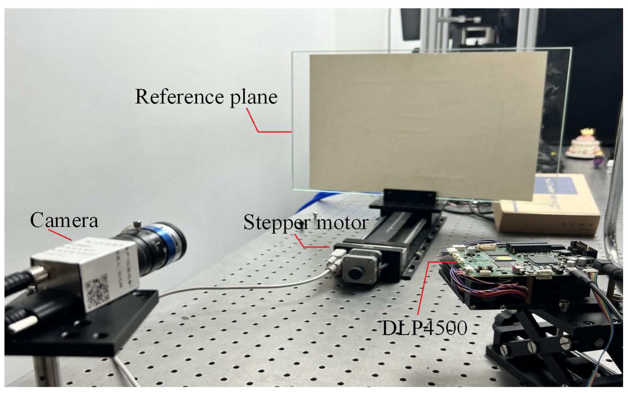
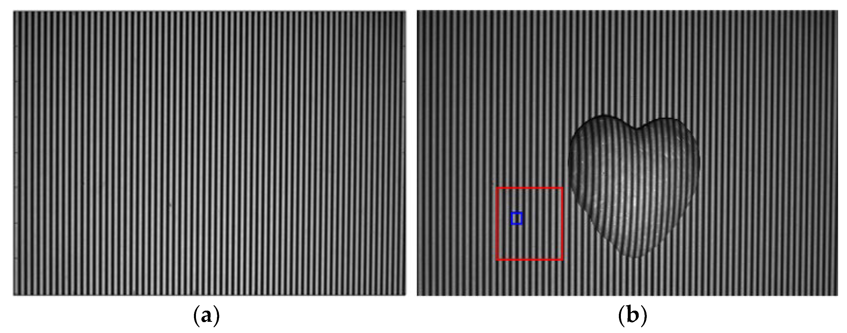
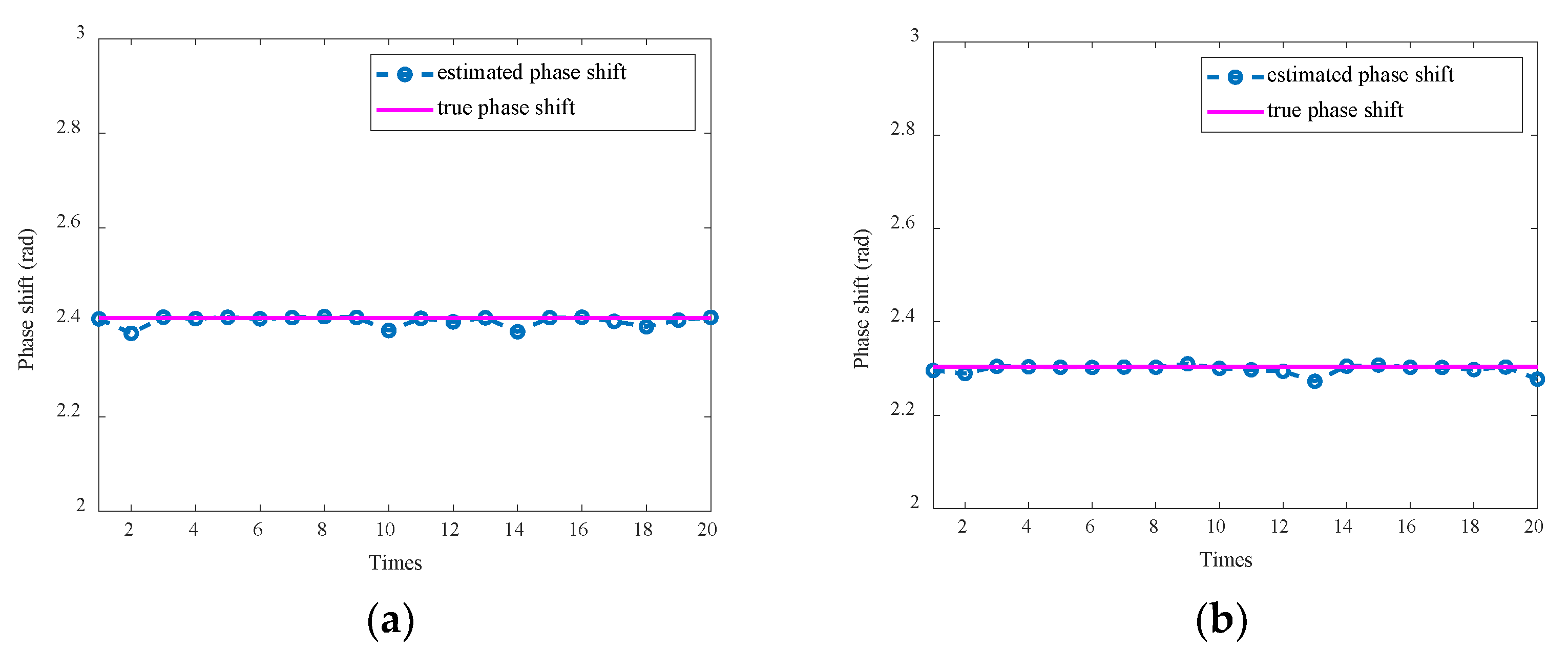
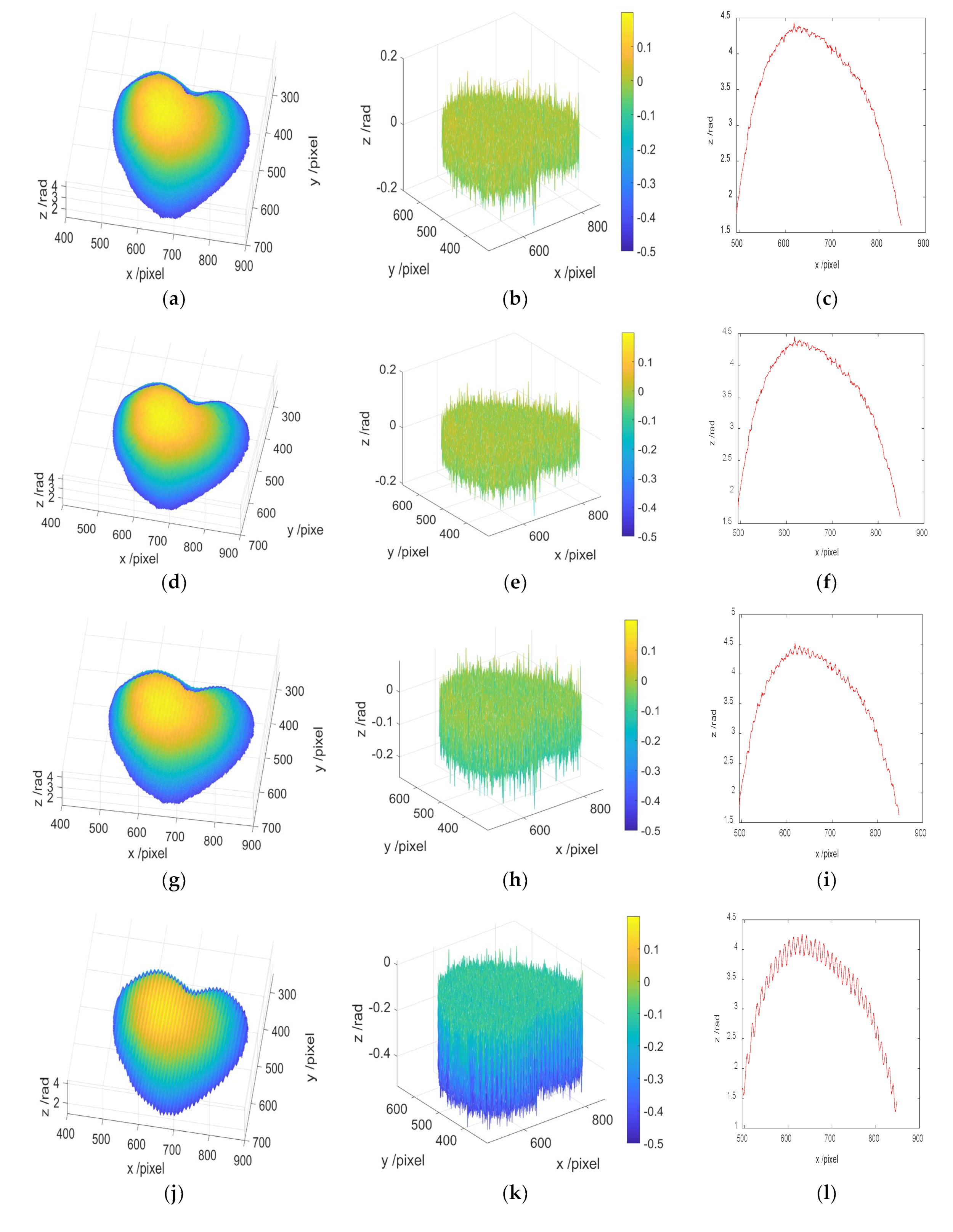
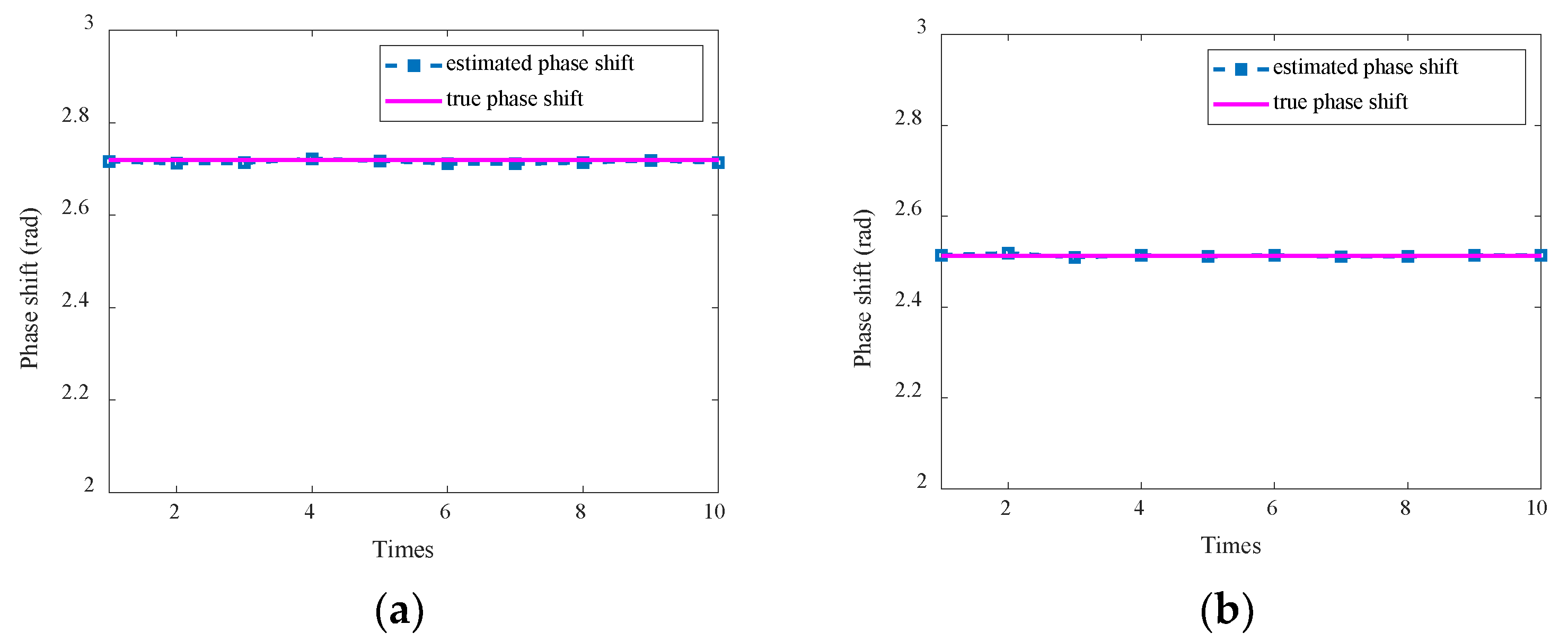
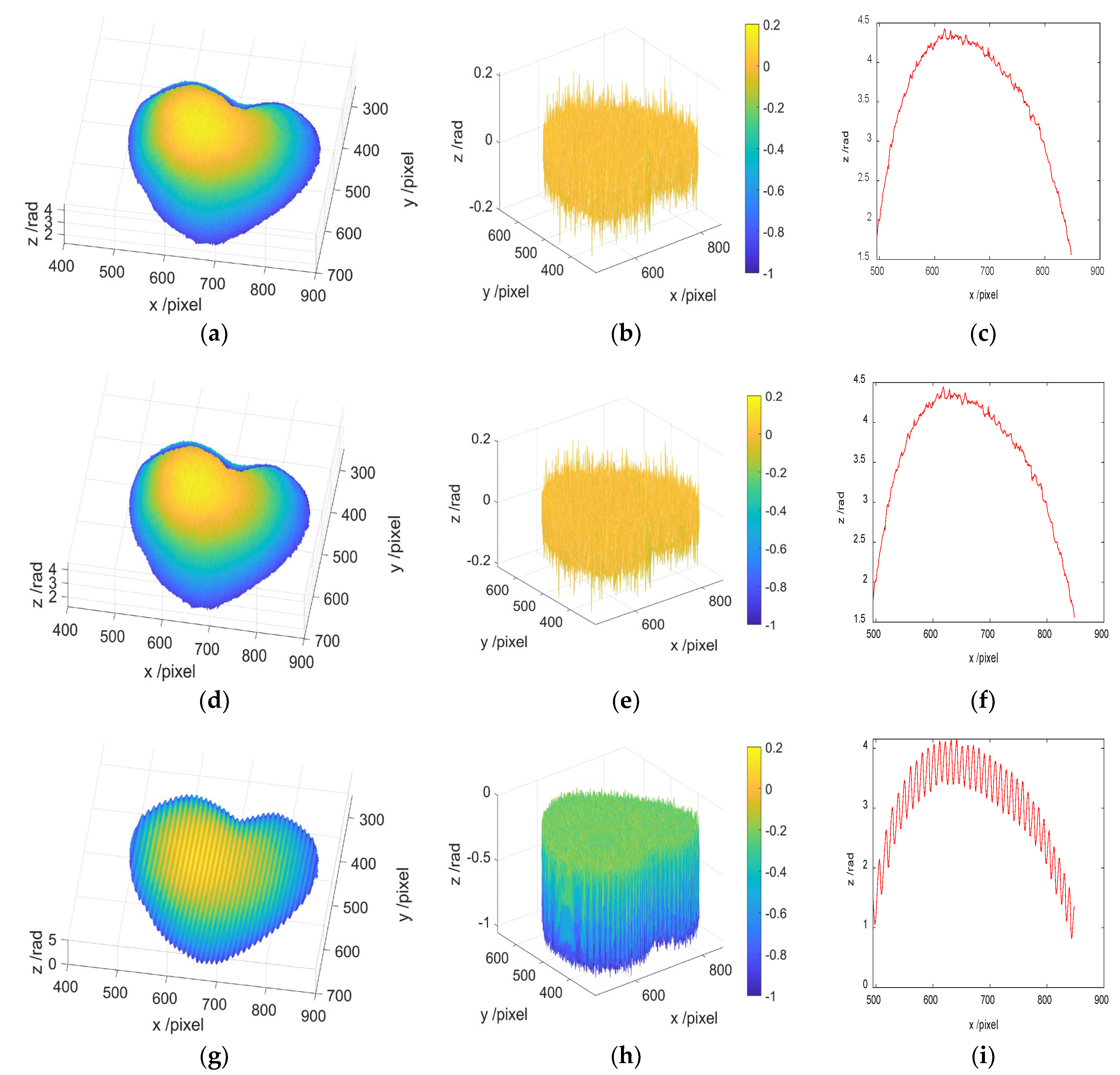
3.1. Experiment on Static Object with Preset Phase Shift Errors

To verify the effectiveness and reliability of the proposed method, the fringes with fixed phase shift and preset additional phase shift errors generated on the computer were projected onto the object, and the fringes were captured by the camera. The proposed method is used to estimate the actual phase shifts in the three-step phase-shifting algorithm, then compare the estimation values to the true phase shift values we preset. A 3-D hardware measuring setup was built to testify the experiment, as shown in Figure 1.

Two cases at different phase shift errors of the fringe patterns are set to perform in the experiment. Smaller and larger extra phase shift errors were considered in the projected fringe patterns in Case I and Case II, respectively. The fixed and manually setup additional phase shift errors of two adjacent frames in the three-step phase-shifting algorithm are, respectively, defined in

Table 1. Parameters used in two cases.

	Phase Shift (rad)	δ1 (rad)	δ2 (rad)	ε1 (rad)	ε2 (rad)	ε3 (rad)	ε2 − ε1 (rad)	ε3 − ε2 (rad)
Case I	2π/3	π/10	π/6	0	2π/3 + π/10	4π/3 + π/6	23π/30 ≈ 2.4086	11π/15 ≈ 2.3038
Case II	2π/3	π/5	π/3	0	2π/3 + π/5	4π/3 + π/3	13π/15 ≈ 2.7189	4π/5 ≈ 2.5133

. In addition, the captured fringe patterns are shown in Figure 2a,b, with the size of 1200 × 1920 pixels being a grayscale with a value of 256 grays. The red and blue boxes represent the selected mask and window, respectively. The selected mask can be on or off the object, which must have the property of linear phase, with the window size of 31 pixels around a selected pixel approximated as the quadratic phase. The actual phase shifts estimated by the proposed algorithm are extracted to substitute into Equation (21), and the wrapped phase can be obtained to reconstruct the full-field phase.

The estimated phase shifts computed at 20-pixel locations in the window are shown in Figure 3 under Case I. It can be observed from Figure 3a,b that all pixels in the window resulted in accurate phase estimates, with the proposed algorithm having consistent accurate phase shift estimation in different pixels within small phase shift errors.

The proposed algorithm is compared with the AIA and traditional three-step phase-shifting algorithm. The estimated phase shifts of two adjacent frames (${\widehat{\epsilon }}_2-{\widehat{\epsilon }}_1$ and ${\widehat{\epsilon }}_3-{\widehat{\epsilon }}_2$) under Case I are 2.4060 rad and 2.2975 rad, respectively, using the proposed algorithm, and the corresponding estimation errors of these phase shifts are 0.0026 rad and 0.0063 rad compared to the truth values shown in Table 1. The results of the AIA greatly depend on the predefined accuracy ϵ [17]. When ϵ = 10⁻⁴ is set, the extracted phase shifts by the AIA are 2.4079 rad and 2.3097 rad, respectively, and the corresponding phase shift errors are 0.0007 rad and 0.0059 rad compared to the truth values. However, the accuracy of the AIA decreases as the preset accuracy decreases, and the higher the preset accuracy, the more iterations and the longer the time. When ϵ = 10⁻¹ is set, the acquired phase shifts using the AIA are 2.4221 rad and 2.3280 rad, respectively, with the estimation accuracy remarkably declining in this preset accuracy. The proposed algorithm shows good estimation ability under a situation of small phase shifts, and the estimated phase shift accuracy using the proposed algorithm achieves good accuracy and efficiency.

The recovered phases, the error distributions, and section line on the 500th row of these retrieved results of the measured object are shown in Figure 4. Taking the twelve-step phase shift as the ground truth, the error distributions are demonstrated in Figure 4b,e,h,k. The restored full-field phases are smoother compared with the standard three-step phase-shifting algorithm. The estimation accuracy can be guaranteed under small phase shift error states, with the error caused by the inaccurate phase shift better eliminated.

For Case II, the estimated phase shifts of two adjacent frames (${\widehat{\epsilon }}_2-{\widehat{\epsilon }}_1$ and ${\widehat{\epsilon }}_3-{\widehat{\epsilon }}_2$) are 2.7168 rad and 2.5118 rad, respectively, and the corresponding estimation errors of these phase shifts are 0.0021 rad and 0.0015 rad, with the averaged estimated phase shift accuracy reached 99.93% compared to the true phase shifts shown in Table 1. It can be concluded that the phase shifts are well estimated exploiting the proposed algorithm under small and large phase shifts, which turns out to be a robust method in evaluating the phase shift. The iteratively obtained phase shifts by the AIA (ϵ = 10⁻⁴) are 2.7231 rad and 2.5254 rad, respectively, and the corresponding phase shift errors are 0.0042 rad and 0.0121 rad compared to the preset value. The reconstructed accuracy of the AIA is slightly lower than that of the proposed algorithm.

The phase shift estimation testing at different times in a mask window is shown in Figure 5a,b. There were 10 measurements used for observation and 20 pixels selected in the window for estimation each time, with the actual phase shift values evaluated from the 20 pixel locations. The estimation of each time provides reliable phase shift values, while the consistency of 10 measurements shows that the algorithm is considered to have good robustness, reliability, and stability.

The retrieved phases, error distributions, and section line on the 500th row of the measured object compared with the twelve-step phase shift are respectively shown in Figure 6. The phase obtained by the proposed algorithm is better reconstructed than that obtained by traditional three-step phase-shifting algorithm, and is superior to the AIA in the case of larger additional phase shift errors. The reconstructed accuracy can be guaranteed even at large phase shift error states, and the phase errors are better removed. The reconstructed efficiency is enhanced by employing the EKF-based estimation method in the PMP system. It can be noted that the proposed algorithm can deal with the estimation of captured fringes with both large and small phase shifts, and achieve good estimation performance, and eliminate the phase errors caused by the inaccurate phase shift.

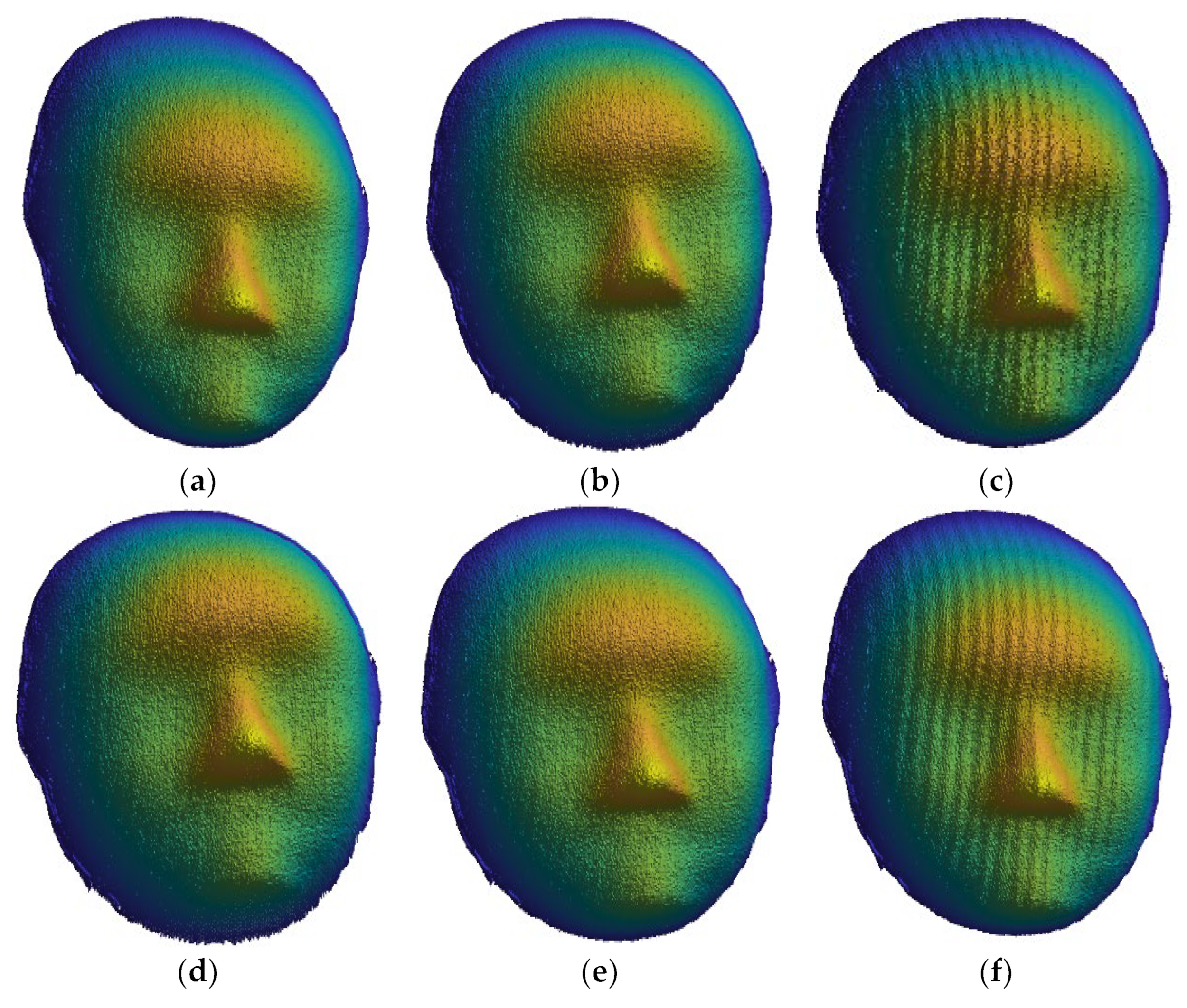
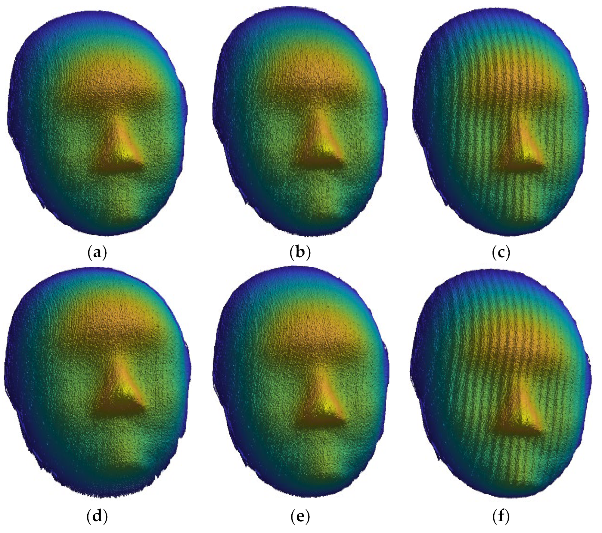
3.2. Experiment on Dynamic Scene with Uncertain Phase Shift Errors

To verify the performance of our method in the dynamic scene, a structure light projection system composed of a DLP projector (LightCrafter 4500) and a camera (Bauma VCXU-31M, 800 × 1200 pixels, maximum sampling speed 300 fps) was built. The rigid object was moving uniformly and non-uniformly along the z-direction towards the camera. The motion of a measured object placed on a flat plate is controlled by a motorized linear translation platform. The moving speed of the translation was 0.25 mm/step, one fringe pattern was projected for each step, and the captured fringe patterns were utilized to reconstruct the object shape. The AIA (ϵ = 10⁻⁴) is employed to provide the reference phase.

Patterns taken at equal intervals are used for uniform motion. The estimated phase shift and designed phase shifts under the uniform motion of the measured object are shown in

Table 2. Estimated phase shifts under different algorithms in uniform motion.

	Uniform Motion				Designed Phase Shifts between Two Frames
	26th Frame		30th Frame
	Proposed	AIA	Proposed	AIA
Phase shift ${\widehat{\epsilon }}_2-{\widehat{\epsilon }}_1$	2.0420	2.0392	2.0424	2.0398	2π/3 ≈ 2.0944
Phase shift ${\widehat{\epsilon }}_3-{\widehat{\epsilon }}_2$	2.0422	2.0388	2.0353	2.0463	2π/3 ≈ 2.0944

. The reconstructed results of the rigid object uniform motions at #26 and #30 are shown in Figure 7. It can be seen from Figure 7c,f that the phase errors induced by the uniform motion distinctly exist in the traditional three-step phase-shifting algorithm, and the proposed method can effectively eliminate the motion ripple and accurately restore the object phase, as shown in Figure 7a,d, and achieve similar reconstructed results to the AIA.

Unequal intervals are employed to carry out the non-uniform motion, with #22 representing the object moving fast and then slow. The values 22, 24, and 25 (i.e., stand for the step numbers of the flat plate in the guide) are selected as the patterns of three-step phase shift, and #30 represents the object moving slow and then fast, 30, 31, and 33 patterns are selected to realize the three-step phase shift. The estimated phase shifts and designed phase shifts under non-uniform motion of the object are shown in

Table 3. Estimated phase shifts under different algorithms in non-uniform motion.

	Non-Uniform Motion				Designed Phase Shifts between Two Frames
	22th Frame		30th Frame
	Proposed	AIA	Proposed	AIA
Phase shift ${\widehat{\epsilon }}_2-{\widehat{\epsilon }}_1$	1.9872	1.9880	2.0414	2.0391	2π/3 ≈ 2.0944
Phase shift ${\widehat{\epsilon }}_3-{\widehat{\epsilon }}_2$	2.0494	2.0479	1.9796	1.9943	2π/3 ≈ 2.0944

. It can be observed from Figure 8 that the proposed method can efficiently remove the phase errors of the object with non-uniform motion caused by the additional phase shift. The phase retrieved results of the object in non-uniform motion have the same effect as those of the object in uniform motion using the proposed method.

The difference in actual phase shift values between two adjacent frames is relatively small under uniform motion. Since the change of phase shift values between frames is no longer a constant in the non-uniform motion, the difference of actual phase shift values between two adjacent frames is relatively large under non-uniform motion. It can be concluded that the fixed designed phase shift of 2/3π rad has varied in the case of the object motion, the unavoidable extra phase shifts result in phase errors, and the actual phase shifts can be evaluated directly by utilizing the proposed EKF estimation method to reduce the motion ripple.

The running time of the proposed algorithm is illustrated in

Table 4. Computational time of the proposed method with different window size.

Stage	Time Cost (s)
	Window Size 31	Window Size 35
Phase shift estimation (region-wise)	0.746	0.911
Wrapping phase (full-field)	6.456	6.562
Unwrapping phase (full-field)	2.073	2.128
Total	9.275	9.601

. The whole processing is run on a computer with Intel Core i7-1165G7 at 2.8 GHz. It can be seen that the operation time increases as the window size increases, due to the fact that the bigger the window size, the more pixels you have to deal with. Since the AIA is an iterative method, the time consumed in phase shift estimation using AIA is 11.636 s (10 iterations), which is higher computational complexity than that of the proposed algorithm. The proposed algorithm is superior to the AIA in speed and efficiency.

4. Discussion

The estimation method based on EKF for uncertain phase shifts in a 3-D shape measurement technique has high speed, high accuracy, and robustness. The proposed algorithm was conducted in the mask window and remarkably reduced the computational time of traditional pixel-wise algorithms and iterative algorithms. Pixels in the selected window were used to evaluate the phase shift, while pixels outside the window did not participate in the estimation, which greatly improved the efficiency of the overall reconstruction. The proposed region-wise estimation method is fast and very suitable for real-time processing in practical applications.

The proposed algorithm can maintain good robustness and highly accurate performance. The iterative algorithm is highly sensitive to the initial or preset parameters and the performance will degrade or fail when the preset values change. Therefore, in this paper, the elimination of the background and fringe modulation from the selected region fringe patterns aims to reduce the estimation parameters and the estimation errors introduced by the background, modulation, and other factors, which greatly improves the robustness and accuracy of the phase shift estimation.

The proposed algorithm is slightly dependent on the selected pixel locations in the mask window. Although the estimated phase steps are a slightly different at different pixels, the evaluated phase shift and the reconstructed results are mostly not sensitive to the selection of pixel locations. However, the proposed algorithm can only be applied in the reconstruction of a mechanical projector device and translational motion due to region-wise estimation, and is not applicable for rotation motion and deformation measurement.

5. Conclusions

In this paper, the region-wise estimation method based on EKF for the uncertain phase shift is proposed to reduce the phase error induced by the imprecise phase shift. The approximation parameters of the quadratic phase function of the adjacent frame in the mask window are employed to evaluate the actual phase shift with the background intensity and fringe modulation removed, and the continuous phase of the object is restored by the spatial unwrapping process from the wrapped phase. This work provides an alternative way to eliminate phase shift errors. Experimental results demonstrate that the proposed method is available and practical for the inaccurate phase shift, and can be used to solve the phase shift error caused by the object motion and mechanical projector.

References

1. Chen, F.; Brown, G.M.; Song, M.M. Overview of three-dimensional shape measurement using optical methods. Opt. Eng. 2000, 39, 10–22. [Google Scholar]
2. Takeda, M.; Mutoh, K. Fourier-transform profilometry for the automatic-measurement of 3-d object shapes. Appl. Opt. 1983, 22, 3977–3982. [Google Scholar] [CrossRef]
3. Zuo, C.; Feng, S.; Huang, L.; Tao, T.; Yin, W.; Chen, Q. Phase shifting algorithms for fringe projection profilometry: A review. Opt. Lasers Eng. 2018, 109, 23–59. [Google Scholar] [CrossRef]
4. Kulkarni, R.; Rastogi, P. Single and Multicomponent Digital Optical Signal Analysis; Estimation of Phase and Its Derivatives; IOP Publishing: Bristol, UK, 2017. [Google Scholar]
5. Zhang, S. High-speed 3D shape measurement with structured light methods: A review. Opt. Lasers Eng. 2018, 106, 119–131. [Google Scholar] [CrossRef]
6. Cheng, Y.-Y.C.; Wyant, J.C. Two-wavelength phase shifting interferometry. Appl. Opt. 1984, 23, 4539–4543. [Google Scholar] [CrossRef]
7. Lu, L.; Suresh, V.; Zheng, Y.; Wang, Y.; Xi, J.; Li, B. Motion induced error reduction methods for phase shifting profilometry: A review. Opt. Lasers Eng. 2021, 141, 106573. [Google Scholar] [CrossRef]
8. Li, B.; Liu, Z.; Zhang, S. Motion-induced error reduction by combining Fourier transform profilometry with phase-shifting profilometry. Opt. Express 2016, 24, 23289–23303. [Google Scholar] [CrossRef]
9. Lu, L.; Jia, Z.; Luan, Y.; Xi, J. Reconstruction of isolated moving objects with high 3D frame rate based on phase shifting profilometry. Opt. Commun. 2019, 438, 61–66. [Google Scholar] [CrossRef]
10. Schwider, J. Phase shifting interferometry: Reference phase error reduction. Appl. Opt. 1989, 28, 3889–3892. [Google Scholar] [CrossRef]
11. Hyun, J.-S.; Chiu, G.T.-C.; Zhang, S. High-speed and high-accuracy 3D surface using a mechanical projector. Opt. Express 2018, 26, 1474–1487. [Google Scholar] [CrossRef]
12. Liu, Y.; Zhang, Q.; Liu, Y.; Yu, X.; Hou, Y.; Chen, W. High-speed 3D shape measurement using a rotary mechanical projector. Opt. Express 2021, 29, 7885–7903. [Google Scholar] [CrossRef]
13. Guo, Y.; Da, F.; Yu, Y. High-quality defocusing phase-shifting profilometry on dynamic objects. Opt. Eng. 2018, 57, 105105. [Google Scholar] [CrossRef]
14. Wu, K.; Li, M.; Lu, L.; Xi, J. Reconstruction of Isolated Moving Objects by Motion-Induced Phase Shift Based on PSP. Appl. Sci. 2021, 12, 252. [Google Scholar] [CrossRef]
15. Cong, P.; Xiong, Z.; Zhang, Y.; Zhao, S.; Wu, F. Accurate dynamic 3d sensing with fourier-assisted phase shifting. IEEE J. Select. Top Sig. Process. 2014, 9, 396–408. [Google Scholar] [CrossRef]
16. Guo, W.; Wu, Z.; Li, Y.; Liu, Y.; Zhang, Q. Real-time 3D shape measurement with dual-frequency composite grating and motion-induced error reduction. Opt. Express 2020, 28, 26882–26897. [Google Scholar] [CrossRef]
17. Wang, Z.; Han, B. Advanced iterative algorithm for phase extraction of randomly phase-shifted interferograms. Opt. Lett. 2004, 29, 1671–1673. [Google Scholar] [CrossRef]
18. Lu, L.; Jiangtao, X.; Yanguang, Y.; Qinghua, G. Improving the accuracy performance of phase-shifting profilometry. Opt. Express 2020, 28, 26882–26897. [Google Scholar]
19. Guo, W.; Wu, Z.; Zhang, Q.; Wang, Y. Real-time motion-induced error compensation for 4-step phase-shifting profilometry. Opt. Express 2021, 29, 23822–23834. [Google Scholar] [CrossRef]
20. Wang, Y.; Liu, Z.; Jiang, C.; Zhang, S. Motion induced phase error reduction using a Hilbert transform. Opt. Express 2018, 26, 34224–34235. [Google Scholar] [CrossRef]
21. Feng, S.; Zuo, C.; Tao, T.; Hu, Y.; Zhang, M.; Chen, Q.; Gu, G. Robust dynamic 3-D measurements with motion-compensated phase-shifting profilometry. Opt. Lasers Eng. 2018, 103, 127–138. [Google Scholar] [CrossRef]
22. Su, W.; Tan, J.; He, Z. A Deep Learning-Based Approach for Motion-Induced Error Reduction in Fringe Projection Profilometry. In Proceedings of the SPIE, Eighth Symposium on Novel Photoelectronic Detection Technology and Applications, Kunming, China, 7–9 December 2021; Volume 12169. [Google Scholar]
23. Yu, H.; Chen, X.; Zhang, Z.; Zuo, C.; Zhang, Y.; Zheng, D.; Han, J. Dynamic 3-D measurement based on fringe-to-fringe transformation using deep learning. Opt. Express 2020, 28, 9405–9418. [Google Scholar] [CrossRef] [PubMed]
24. Li, Y.; Guo, W.; Shen, J.; Wu, Z.; Zhang, Q. Motion-Induced Phase Error Compensation Using Three-Stream Neural Networks. Appl. Sci. 2022, 12, 8114. [Google Scholar] [CrossRef]
25. Han, L.; Li, Z.; Zhong, K.; Cheng, X.; Luo, H.; Liu, G.; Shang, J.; Wang, C.; Shi, Y. Vibration detection and motion compensation for multi-frequency phase-shifting-based 3D sensors. Sensors 2019, 19, 1368. [Google Scholar] [CrossRef] [PubMed]
26. Liu, Z.; ZIBLEY, P.C.; Zhang, S. Motion-induced error compensation for phase shifting profilometry. Opt. Express 2018, 26, 12632–1263762. [Google Scholar] [CrossRef]
27. Wu, Z.; Guo, W.; Zhang, Q. Two-frequency phase-shifting method vs. Gray-coded-based method in dynamic fringe projection profilometry: A comparative review. Opt. Lasers Eng. 2022, 153, 106995. [Google Scholar] [CrossRef]
28. Choi, H.; Park, J.; Yang, Y.-M. A Novel Quick-Response Eigenface Analysis Scheme for Brain and Computer Interfaces. Sensors 2022, 22, 5860. [Google Scholar] [CrossRef]
29. Lai, X.; Zhu, G.; Chambers, J. A fuzzy adaptive extended Kalman filter exploiting the Student’s t distribution for mobile robot tracking. Meas. Sci. Technol. 2021, 32, 105017. [Google Scholar] [CrossRef]
30. Simon, D. Optimal State Estimation: Kalman, H Infinity, and Nonlinear Approaches; John Wiley and Sons: Hoboken, NJ, USA, 2006. [Google Scholar]
Figure 1. Experimental hardware measuring system setup.
Photonics 10 00207 g001
Figure 2. First frame of three-step phase-shifting fringe pattern on the surface of (a) the reference plane and (b) the measured object in Case I and Case II.
Photonics 10 00207 g002
Figure 3. Estimated phase shifts of (a) ε ^ 2 ε ^ 1 and (b) ε ^ 3 ε ^ 2 under Case I.
Photonics 10 00207 g003
Figure 4. Experimental results of the measured object under Case I. (a) Reconstructed phase, (b) error distribution, (c) section line on the 500th row by the proposed algorithm; (d) reconstructed phase, (e) error distribution, (f) section line on the 500th row by the AIA (ϵ = 10−4); (g) reconstructed phase, (h) error distribution, (i) section line on the 500th row by the AIA (ϵ = 10−1); (j) reconstructed phase, (k) error distribution, (l) section line on the 500th row by the traditional three-step phase-shifting algorithm.
Photonics 10 00207 g004
Figure 5. Estimated phase shifts of (a) ε ^ 2 ε ^ 1 and (b) ε ^ 3 ε ^ 2 under Case II.
Photonics 10 00207 g005
Figure 6. Experimental results of the measured object under Case II. (a) Reconstructed phase, (b) error distribution, (c) section line on the 500th row by the proposed algorithm; (d) reconstructed phase, (e) error distribution, (f) section line on the 500th row by the AIA (ϵ = 10−4); (g) reconstructed phase, (h) error distribution, (i) section line on the 500th row by the traditional three-step phase-shifting algorithm.
Photonics 10 00207 g006
Figure 7. Experiment results of an object with uniform motion. (a) Reconstructed result of 26 frame: the proposed algorithm; (b) Reconstructed result of 26 frame: the AIA (ϵ = 10−4); (c) Reconstructed result of 26 frame: the traditional three-step phase-shifting algorithm; (d) Reconstructed result of 30 frame: the proposed algorithm; (e) Reconstructed result of 30 frame: the AIA (ϵ = 10−4); (f) Reconstructed result of 30 frame: the traditional three-step phase-shifting algorithm.
Photonics 10 00207 g007
Figure 8. Experiment results of an object with non-uniform motion. (a) Reconstructed result of 22 frame: the proposed algorithm; (b) Reconstructed result of 22 frame: the AIA (ϵ = 10−4); (c) Reconstructed result of 22 frame: the traditional three-step phase-shifting algorithm; (d) Reconstructed result of 30 frame: the proposed algorithm; (e) Reconstructed result of 30 frame: the AIA (ϵ = 10−4); (f) Reconstructed result of 30 frame: the traditional three-step phase-shifting algorithm.
Photonics 10 00207 g008