Movable Optical Frequency Ruler with Optical Activity

Abstract

Optical frequency rulers (OFR) are suggested for use as optical wavelength or frequency references for spectra manipulation or unknown wavelength measurement. In the past, complicated mechanisms that are not easy to utilize were used to make OFR, such as a double-slits with a high-speed fluid or an external circuit to control the liquid crystal birefringence. This work introduces a simple structure to produce an OFR, which should be easier to implement. It utilizes quartz block optical activity and two polarizers. Because of the strong wavelength dependence of the rotatory power, each wavelength component in the spectrum experiences a different amount of polarization angle rotation. Some components whose angles are perpendicular to that of the analyzer are filtered out and naturally form the OFR’s ticks. The numerical results show that those spectral ticks can be moved to higher or lower wavelengths by rotating the analyzer’s angle. This scheme provides another possibility for creating movable OFR with the merit of easy usage.

1. Introduction

The study of polychromatic wave diffraction began in the mid 1980′s [1,2] and many important results were found, such as the singular optics in polychromatic light [3,4]; the spatial and spectral correspondence relationship [5]; and some applications including spectra manipulation with the photorefractive effect [6], spectral switches [7,8], and Talbot spectra [9] were proposed. It was also found that when a polychromatic light passes through a double slit, the interfered or diffracted spectrum detected in the far-field changes substantially. It contains many peaks and valleys (dark lines), and it follows the interference law [10]. Those lines are wavelengths satisfying destructive interference and they vanish in the output spectrum. One of the authors, Han, suggested that those disappearing wavelengths are components that could be used as optical wavelength (or frequency) references, as long as their positions are known exactly. It was named an “optical frequency ruler” because those dark lines work like a ruler’s ticks. In the past, similar reference lines were usually produced by the Fabry–Perot etalon or optical comb techniques with a resonant cavity [11,12]. Two more optical frequency ruler schemes were proposed without cavities, utilizing a moving fluid [13] and liquid crystal birefringence, [14,15] respectively. However, in the former, the required high fluid speed is difficult to reach. In the latter, an external circuit is needed to control the liquid crystal orientation. In this work, we present another method to produce an optical frequency ruler phenomenon, without using those mechanisms. By employing the optical activity of a solid material and two polarizers, this phenomenon naturally shows up and can be controlled by simply rotating one of the polarizer’s angles.

The structure of this work is as follows. Section 1 is the introduction. The theory, configuration, and numerical results are included in Section 2. Section 3 is the conclusions and discussion.

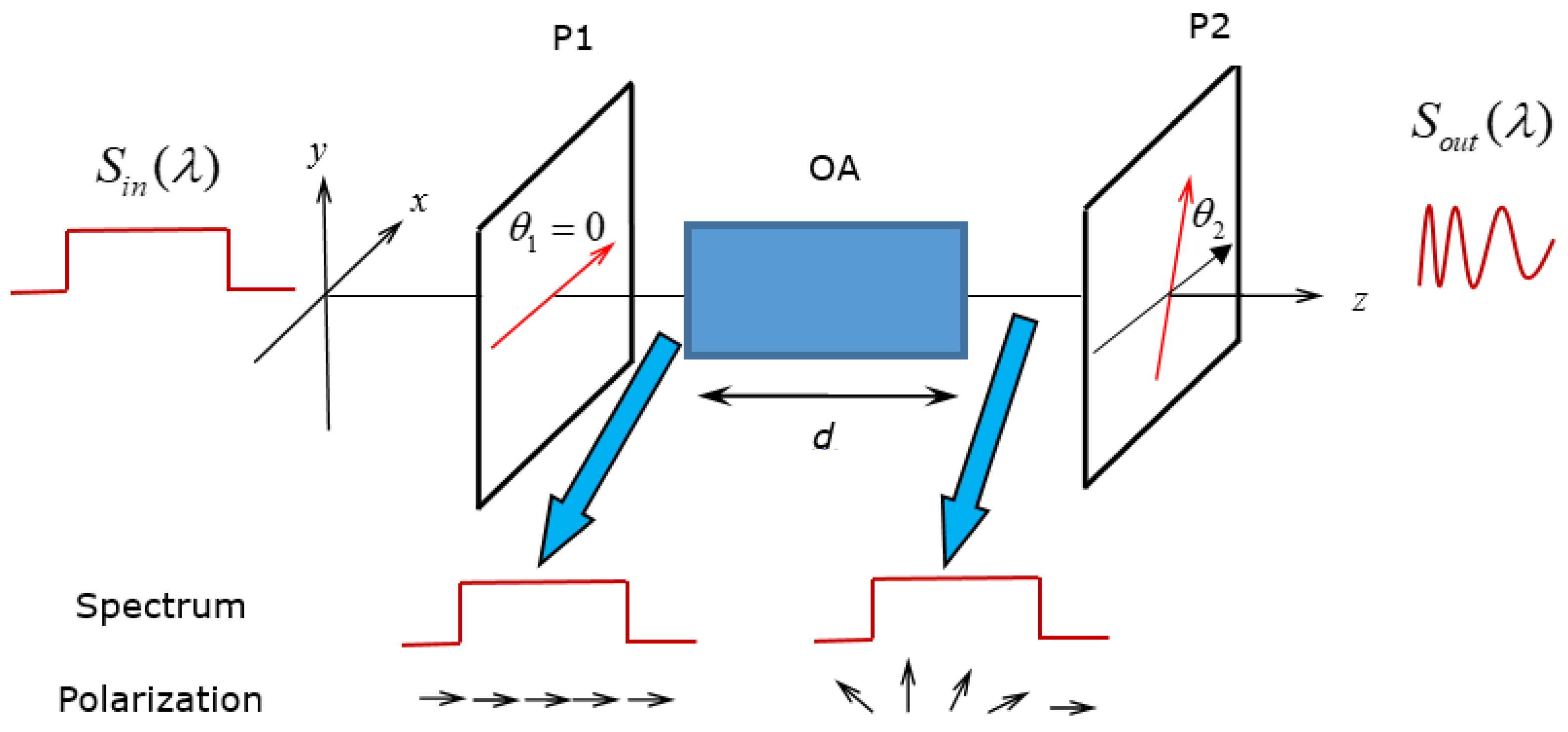
2. Theory and Numerical Results

Optical activity exists in some materials which act as natural polarization rotators. The two normal modes are right- and left-circularly polarized waves. Usually, the refraction index of an optically active medium is described as $n_{+}$ and $n_{-}$ for the right and left circular polarization waves, respectively. The rotatory power $\rho$ (rotation angle per unit length) is [16]

$$\rho =\frac{\pi }{\lambda }\left(n_{+}-n_{-}\right)$$

(1)

where $\lambda$ is the wavelength in vacuum. Thus, a linearly polarized wave travels in the material with thickness d, the angle of polarization rotation $\varphi$ is

$$\varphi =\rho \cdot d=\frac{\pi d}{\lambda }\left(n_{+}-n_{-}\right) .$$

(2)

If $n_{+}< n_{-}$, $\rho$ is positive; such materials are said to be dextrorotary, whereas those for which $n_{+}> n_{-}$ are termed levorotary.

As we show below, this polarization rotating ability can be used as an intensity modulator for a monochromatic wave and an optical frequency ruler for a polychromatic wave.

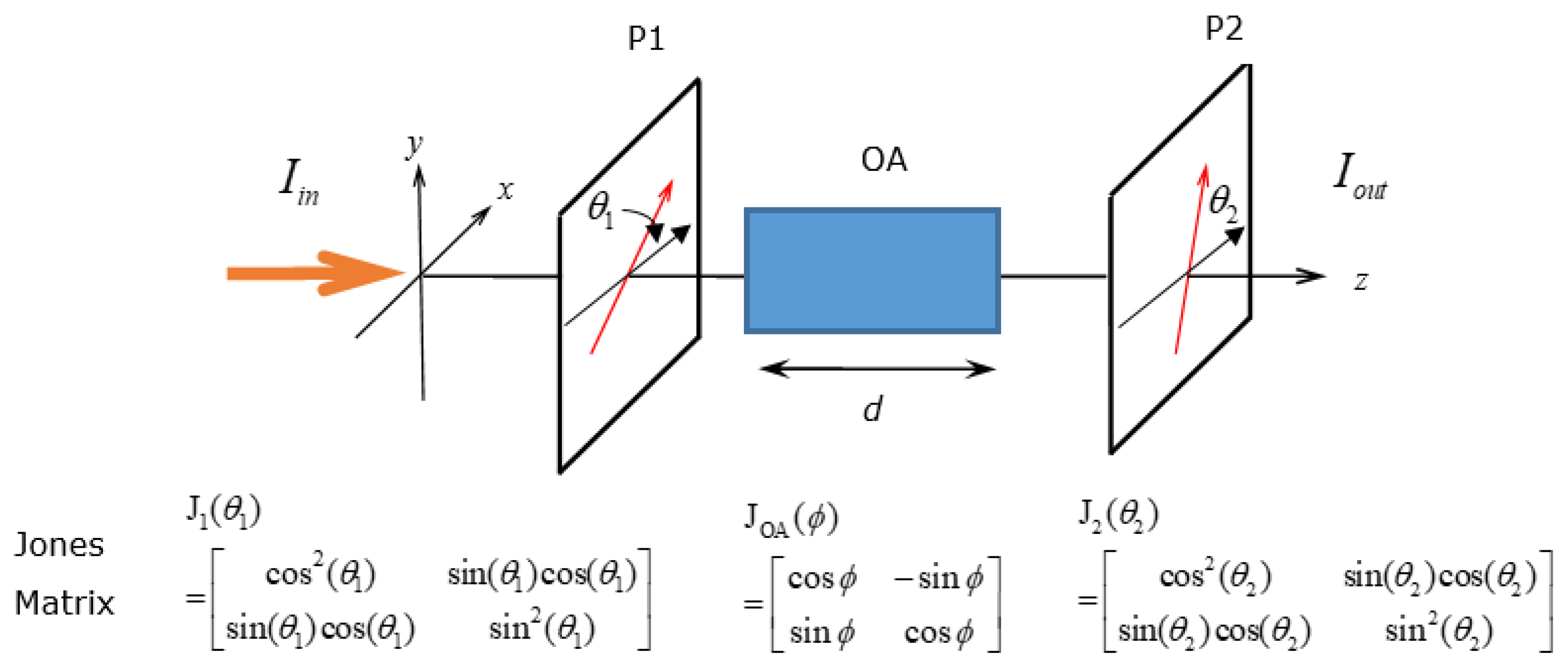
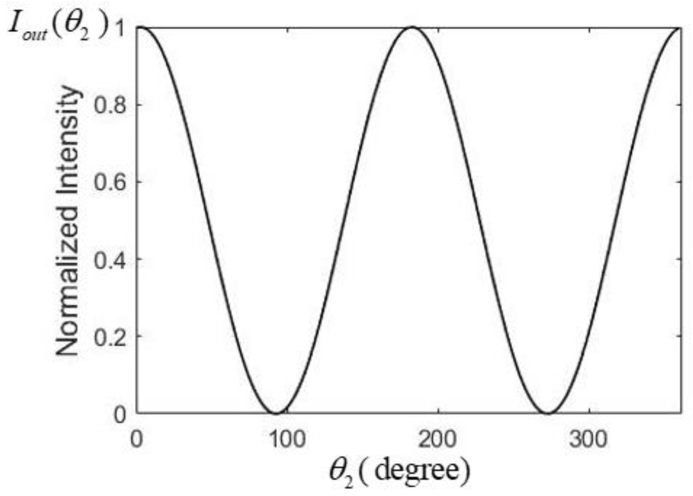
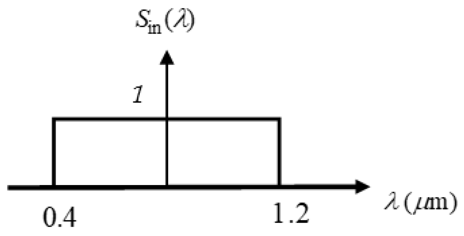
2.1. Monochromatic Wave Situation

Consider the configuration shown in Figure 1. There is an optically active material placed between two polarizers P1 and P2 with polarization angles ${\theta }_1$ and ${\theta }_2$ (with respect to x axis) respectively. As indicated below the figure, the polarization states can be described as Jones vectors and Jones matrixes [17]. The three Jones matrixes are named J₁, J_OA, and J₂, respectively for P1, optically active material, and P2. For an incident wave field with Jones vector ${\stackrel{\rightharpoonup }{E}}_{in}$, the output field ${\stackrel{\rightharpoonup }{E}}_{out}$ is described by

$${\stackrel{\rightharpoonup }{E}}_{out}={\mathrm{J}}_2\cdot {\mathrm{J}}_{\mathrm{OA}}\cdot {\mathrm{J}}_1{\stackrel{\rightharpoonup }{E}}_{in}$$

(3)

Without losing generality and for simplicity, we set ${\stackrel{\rightharpoonup }{E}}_{in}$ being linearly polarized along the x axis with the components $E_x$ and ${\theta }_1$ being 0. Substituting these two conditions into Equation (3), ${\stackrel{\rightharpoonup }{E}}_{out}$ is

$${\stackrel{\rightharpoonup }{E}}_{out}({\theta }_1=0)=\left[\begin{array}{c}\cos ({\theta }_2)\cdot \cos ({\theta }_2-\varphi )\\ \sin ({\theta }_2)\cdot \cos ({\theta }_2-\varphi )\end{array}\right]E_x$$

(4)

Thus, the final output intensity $I_{out}={\stackrel{\rightharpoonup }{E}}_{out}\cdot {\stackrel{\rightharpoonup }{E}}_{out}$ is

$$I_{out}({\theta }_2\hspace{0.17em},\varphi ,\lambda )=\left\{{\left[\cos ({\theta }_2)\cdot \cos ({\theta }_2-\varphi )\right]}^2+{\left[\sin ({\theta }_2)\cdot \cos ({\theta }_2-\varphi )\right]}^2\right\}{I}_{in}$$

(5)

where $I_{in}={\stackrel{\rightharpoonup }{E}}_{in}\cdot {\stackrel{\rightharpoonup }{E}}_{in}=E_x{}^2$ is the incident intensity. Here we intentionally include three letters in the parenthesis of $I_{out}({\theta }_2,\varphi ,\lambda )$ in this order and explain it using the following. The first letter ${\theta }_2$ is a variable indicating the polarization angle of P2; while other two letters $\varphi (=\rho \cdot d)$ and $\lambda$ are parameters which are set by the material (and its thickness) and the operating wavelength selected. Note that the rotatory power $\rho$ itself is wavelength dependent. Quartz (fused silica) is used as an example. The rotatory power is $\rho$ = 7.315 degree/mm at $\lambda$ = 1.0 μm [18]. Figure 2 shows the normalized output intensity $I_{out}({\theta }_2\hspace{0.17em})$ for d = 25 mm ($\varphi =\rho \cdot d$ = 183°) at that wavelength. Here we neglect the Fresnel loss, which can be fairly accounted for by applying a suitable anti-reflection coating on both sides of the quartz block.

The output intensity can be controlled by rotating the polarization angle of P2. Certainly, similar intensity control can be achieved using two polarizers without optically active materials. Usually, this scheme is performed to measure the concentration of some chiral molecular solutions, such as amino acids and sugars. For example, by measuring the rotary power (or equivalently the polarization rotation angle $\varphi$), the optical activity can be obtained. The concentration of the sugar solution is then calculated, which is the principle of saccharimeters. Here a solid quartz material is used just for illustration convenience. Some useful equations in monochromatic form are acquired for later use. This will become obvious for polychromatic spectrum control, as discussed in Section 2.2.

It is interesting to point out another possibility to create intensity modulation. Since the rotatory power $\varphi (=\rho \cdot d)$ depends on the distance traveling in the quartz, the distance can be altered by rotating the quartz block. As shown in Figure 3, assuming the block rotates along the x axis and its normal vector $\hat{\mathrm{N}}$ makes an angle $\eta$ with the z axis. The incident light (the horizontal red line) is incident to the angle $\eta$ upon the quartz’s left interface. Using Snell’s law, the refraction angle ${\eta }^{\prime }{=\sin }^{-1}\left[{\mathrm{n}}^{-1} \sin (\eta )\right]$ is found, where $\mathrm{n}$ is the quartz’s refraction index ($\mathrm{n}=1.462$ at $\lambda$ = 0.5 μm). Thus, the traveling distance inside the block is $d^{\prime }=d/\cos {\eta }^{\prime }$. Figure 4 shows the $I_{out}(\eta )$ for ${\theta }_1=0°,{\theta }_2=90°$, and d = 25 mm at $\lambda$ = 0.5 μm. Note that $\rho$ = 30.84 degree/mm at $\lambda$ = 0.5 μm, which is about four times the value at $\lambda$ = 1.0 μm. Figure 4 shows the normalized output intensity for the $\eta$ interval of [0°, 60°]. Comparing Figure 4 with Figure 2, we find that the two curves exhibit different behavior.

2.2. Polychromatic Wave Situation

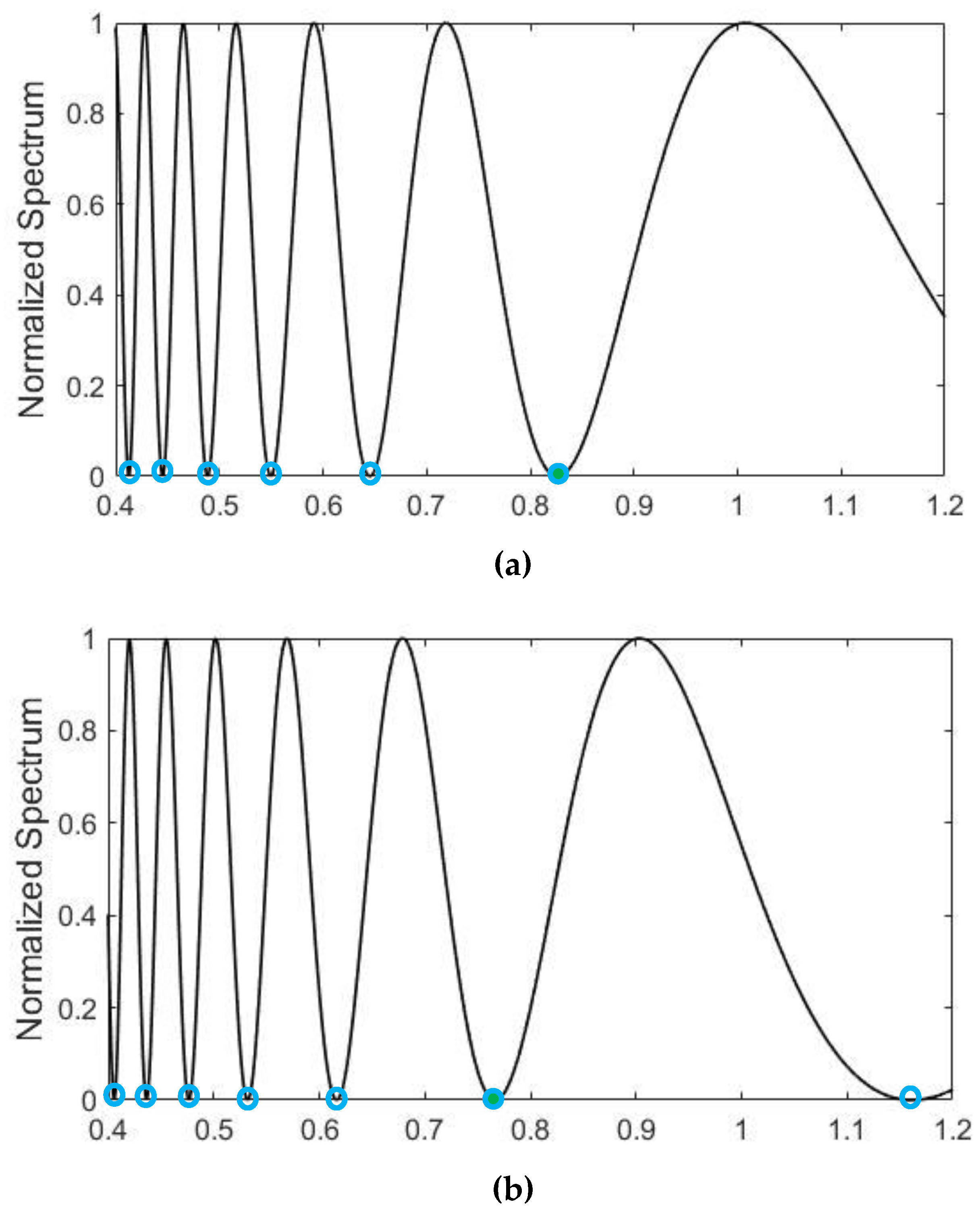
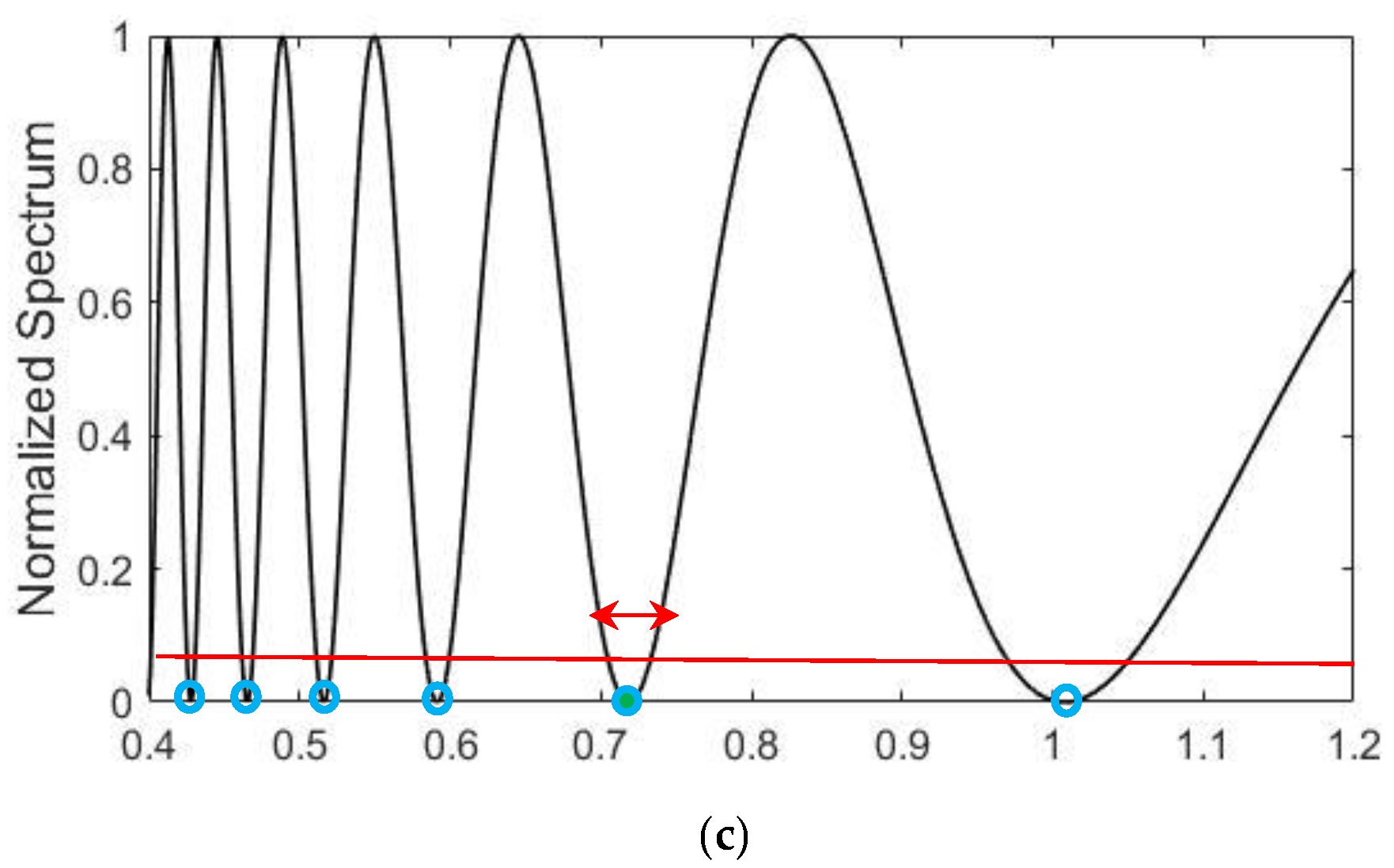
After studying the intensity modulation for a monochromatic wave case, we turn our attention to a polychromatic one. We already know that the refraction index depends on the wavelength (so called the dispersion), but when it comes to the optical activity, the strong rotary power wavelength dependence $\rho$ is dominant. Basically, $\rho$ is approximately inversely proportional to the square of $\lambda$. This property can be traced back to material equations [16] and we have $\rho \left(\lambda \right)\approx 2{\pi }^2\xi /n\left(\lambda \right){\lambda }^2$, where $\xi$ is a pseudo scalar. Note that $\rho \left(\lambda \right)$ also depends on $n\left(\lambda \right)$. In order to give a full description and correct numerical calculations, the following two formulas are used for $\rho \left(\lambda \right)$ and $n\left(\lambda \right)$, which are verified empirically and adapted from the literature [18,19]. Figure 5 shows the behavior of $\rho \left(\lambda \right)$ and $n\left(\lambda \right)$ for quartz in the wavelength range from 0.5 to 1.0 μm. The much larger value change extent for $\rho \left(\lambda \right)$ than that of $n\left(\lambda \right)$ is obvious.

$$\rho (\lambda )=\frac{7.19{\lambda }^2}{{\left({\lambda }^2-0{.09263}^2\right)}^2}$$

(6)

$$n(\lambda )={\left[1 + \frac{0.6962{\lambda }^2}{{\lambda }^2-0{.06840}^2} + \frac{0.4079{\lambda }^2}{{\lambda }^2-0{.1164}^2} + \frac{0.8975{\lambda }^2}{{\lambda }^2-9{.8962}^2}\right]}^{1/2}.$$

Consider an incident polychromatic spectrum $S_{\mathrm{in}}(\lambda )$ with a flat-top distribution ranging from $0.4 \mathsf{\mu }\mathrm{m}$ to $1.2 \mathsf{\mu }\mathrm{m}$, as shown in Figure 6. Here we use $S_{\mathrm{in}}(\lambda )$ to differentiate from ${\stackrel{\rightharpoonup }{E}}_{in}$ because the latter is for the monochromatic situation and the former is for the polychromatic one. The normalization procedure is practiced in Figure 6 because the input intensity can be changed easily. Note that the absorption coefficient of quartz is very low in this spectral range, thus the material absorption can be ignored. Now, because each wavelength component experiences various rotatory power $\rho \left(\lambda \right)$, the final rotation angle $\varphi (\lambda ) = \rho \left(\lambda \right)\cdot d$ is also different, as shown schematically in Figure 7. Using the superposition principle and with the help of Equation (5), the output spectrum at each wavelength $S_{\mathrm{out}}(\lambda , {\theta }_2, \varphi )$ is

$$S_{\mathrm{out}}(\lambda \hspace{0.17em},\varphi (\lambda ),{\theta }_2)=\left\{{\left[\cos ({\theta }_2)\cdot \cos ({\theta }_2-\varphi (\lambda ))\right]}^2+{\left[\sin ({\theta }_2)\cdot \cos ({\theta }_2-\varphi (\lambda ))\right]}^2\right\}{S}_{in}(\lambda )$$

(7)

.

When comparing it with Equation (5) note that now the first letter $\lambda$ in the parenthesis of $S_{\mathrm{out}}(\lambda , \varphi , {\theta }_2)$ is a variable while other two letters $\varphi (\lambda \left)\right(=\rho \left(\lambda \right)\cdot d)$ and ${\theta }_2$ are parameters, which are set by the material (and its thickness) and the polarization angle of P2. Figure 8a–c shows the $S_{\mathrm{out}}\left(\lambda \right)$ for ${\theta }_2=0°, 45°, \mathrm{and} 90°$, respectively, with ${\theta }_1=0°$, and d = 25 mm in the wavelength interval of $S_{\mathrm{in}}(\lambda )$.

We can see from all figures there are many peaks and valleys and some wavelengths indicated by blue circles (or dots) vanish. It is interesting to see if these vanishing wavelengths can be found analytically. After simplifying Equation (7), it is found that the following condition must be satisfied: ${\theta }_2-\varphi (\lambda )=[\mathrm{m}+(1/2)]\pi$, m = 0, 1, 2, 3. However, since $\varphi (\lambda )=\rho \left(\lambda \right)\cdot d$ and Equation (6), after the expansion, it is a quartic polynomial function, which does not have an analytical formula or solution. As explained in Figure 7, these wavelength components are those with a polarization direction vertical to P2 polarizer and are filtered out. These vanishing wavelengths (or dark lines) in the continuous spectrum can be used as wavelength references because their positions are well defined. As mentioned in the introduction, one of the authors Han named this effect an optical frequency ruler since those lines are like the ticks of a ruler, which can help determine an unknown optical frequency or wavelength. However, as seen from Figure 8a, the spacing between the ticks is not regular due to the nonlinear wavelength dependence of the rotary power. The spacing is becomes bigger for larger wavelengths. Also note that the modulated spectrum $S_{\mathrm{out}}(\lambda ,\varphi ,{\theta }_2)$ and the frequency ruler can be controlled by the polarization angle of P2. Comparing Figure 8a (${\theta }_2=0°$) with Figure 8b (${\theta }_2=45°$) and Figure 8c (${\theta }_2=90°$), the rotation of P2 causes the output spectrum to move to the left. To see this clearer, we used a solid blue dot at $\lambda =0.82$ μm in Figure 8a. It moves to $\lambda =0.77$ and $\lambda =0.71$ μm in Figure 8b,c, respectively. Thus, this ruler’s ticks are movable by controlling the P2 polarization angle. This property is advantageous to determining an unknown wavelength. When it falls between two ticks, we can identify it by moving one of the adjacent ticks on it through rotating ${\theta }_2$.

3. Results

In this work we presented a scheme using optical activity to manipulate an incident spectrum. Its configuration consists of two polarizers and one optically active material, a solid quartz sample being used here. First, the monochromatic case is studied. By setting a specific wavelength and knowing the rotatory power at that wavelength, the rotation angle of the polarization can be derived with the Jones matrix. We suggested two ways to control the output intensity, by rotating a second polarizer angle and by rotating the quartz block. The intensity modulation behaves differently for these two methods.

The polychromatic situation can be obtained by superposing various wavelength components. As the results show, for a flat top incident spectrum the modulated output spectrum is directly related to the modulated monochromatic intensity. However, the strong rotary power wavelength dependence and the material dispersion should be carefully considered. Verified empirical relations for these two factors are used in this work. The interpretation of the modulated intensity and the spectrum are different. In the former, the variable is the P2 polarization angle, and in the latter it is the wavelength. Finally, with the formula and numerical examples, we illustrated successfully the optical frequency ruler phenomenon. Those vanishing wavelengths act as the ruler’s ticks which can be used as references for measuring an unknown wavelength. Moreover, we showed that those ticks can be moved by rotating the P2 polarization angle, a movable optical frequency ruler as the title suggested. The advantages of this scheme are its compact configuration and ease of implementation, compared with those using resonant cavities or those needing external circuits to control the liquid crystal’s birefringence. This study contributes one more easy way to offer an optical frequency ruler effect, which may find applications in spectroscopy or spectra manipulations.

4. Discussion

As presented in the last section, this work proposes an OFR scheme with optical activity for an unknown wavelength determination. It is worth presenting the measurement configuration and discussing its accuracy. As shown in the Figure 9 below, a Y-coupler is used to couple the unknown wavelength source and the optical frequency ruler (OFR) source, say, with the spectral distribution as in Figure 8b or Figure 8c. After coming out of the fiber end, a lens is use to collimate the light beam and a dispersive element (prism or grating) is used to disperse the spectrum. A white paper can be placed at the observation plane, and the spread spectrum blow-up on the paper is plotted schematically below. For simplicity, we only plot the visible light band, from 0.4 to 0.8 μm, that is, from purple to red. Now we turn our attention to that blow-up. We plot the colored continuous spectrum in the middle and the unknown source is shown as a long bright orange line. The upper part is the spectrum similar to Figure 8b, with black–white grey tones to indicate spectral variations (i.e., those peaks and valleys in the spectrum). We also use some black lines at the locations of valleys’ minimum to indicate the ticks of OFR. As seen in Figure 8b, the tick closest to 0.8 μm (red end) is at 0.77 μm, which corresponds to the right most of dark line, as indicated by a blue arrow on the top of blow-up of Figure 9. In order to measure the unknown bright orange wavelength more precisely, we can rotate the polarizer P2, to ${\theta }_2=90°$, until that tick coincides with the unknown wavelength, then we know the wavelength at 0.71 μm, as shown in Figure 8c.

It seems that the accuracy depends on how exactly the tick (dark line) can be coincided with the unknown wavelength. It is reasonable to assume that the unknown one can be safely placed in the wavelength width for the dark line intensity varying from 0 to 10% of the peak, as the red line interval in Figure 8c shows. In this case, the accuracy is around ±10 nm. Note that this interval width varies with the wavelength because of the nonlinearity of the spectrum distribution; it decreases with the decreasing of the wavelength. Thus, the accuracy is better for determining a smaller unknown wavelength. If the broader range is wanted, a linear array detector can be placed at the observation plane to record the positions of spectral distribution and the measurement process is the same. For example, a silicon-based CCD has spectral response from 0.4 to 1.1 μm. Thus, the benefit of this scheme lies in that a spectrometer is not required for the wavelength measurement by using this movable OFR method.

References

1. Wolf, E. Invariance of the spectrum of light on propagation. Phys. Rev. Lett. 1986, 56, 1370–1372. [Google Scholar] [CrossRef] [PubMed]
2. Wolf, E. Red shifts and blue shifts of spectral lines emitted by two correlated sources. Phys. Rev. Lett. 1987, 58, 2646–2648. [Google Scholar] [CrossRef] [PubMed]
3. Visser, T.D.; Wolf, E. Spectral anomalies near phase singularities in partially coherent focused wavefields. J. Opt. A Pure Appl. Opt. 2003, 5, 371–373. [Google Scholar] [CrossRef]
4. Soskin, M.S.; Vasnetov, M.V. Singular optics. In Progress in Optics; Wolf, E., Ed.; Elsevier: Amsterdam, The Netherlands, 2001; Volume 42, pp. 219–276. [Google Scholar]
5. Han, P. Spatial–Spectral Correspondence Relationship for Mono—Poly chromatic Light Diffraction. In Progress in Optics; Visser, T.D., Ed.; Elsevier: Amsterdam, The Netherlands, 2018; Volume 63, pp. 33–87. [Google Scholar]
6. Hsu, H.C.; Han, P. Spectra manipulation with the photorefractive effect via the spatial–spectral correspondence relationship. J. Opt. Soc. Am. A 2020, 37, 219–224. [Google Scholar] [CrossRef] [PubMed]
7. Ding, P.; Pu, J.; Weng, J.; Han, P. Spectral anomalies by superposition of polychromatic Gaussian beam and Gaussian vortex beam. Opt. Express 2014, 22, 213037. [Google Scholar] [CrossRef] [PubMed]
8. Foley, J.T.; Wolf, E. Phenomenon of spectral switches as a new effect in singular optics with polychromatic light. J. Opt. Soc. Am. A 2002, 19, 2510–2516. [Google Scholar] [CrossRef] [PubMed]
9. Han, P. Spectra restoration of a transmissive periodic structure in near-field diffraction (Talbot spectra). J. Opt. Soc. Am. A 2015, 32, 1076–1083. [Google Scholar] [CrossRef] [PubMed]
10. Born, M.; Wolf, E. Principles of Optics, 7th ed.; Cambridge University: Cambridge, UK, 1999; p. 587. [Google Scholar]
11. Bartels, A.; Heinecke, D.; Diddams, S.A. 10-GHz self-referenced optical frequency comb. Science 2009, 326, 681. [Google Scholar] [CrossRef] [PubMed]
12. Kuhn, K.J. Laser Engineering; Prentice-Hall Inc.: Hoboken, NJ, USA, 1998; Chapter 3. [Google Scholar]
13. Han, P. Optical frequency ruler with moving fluid. Chin. Opt. Lett. 2013, 11, 122601. [Google Scholar] [CrossRef]
14. Kanseri, B.; Gyaprasad, A.K.R. Broadband spectral shaping using nematic liquid crystal. Results Phys. 2019, 12, 531–534. [Google Scholar] [CrossRef]
15. Ding, P.F.; Hsu, H.C.; Han, P. Spectral manipulation and tunable optical frequency ruler using liquid crystal’s birefringence. OPTIK 2019, 179, 115–121. [Google Scholar] [CrossRef]
16. Teich, M.; Saleh, B. Fundamentals of Photonics, 2nd ed.; Wiley: New York, NY, USA, 2007; p. 228. [Google Scholar]
17. Iizuka, K. Elements of Photonics; Wiley: New York, NY, USA, 2002; Volume 1, p. 421. [Google Scholar]
18. Chandrasekhar, S. The optical rotatory power of quartz and its variation with temperature. Proc. Indian Acad. Sci. A 1952, 35, 103–113. [Google Scholar] [CrossRef]
19. Malitson, I.H. Interspecimen comparison of the refractive index of fused silica. J. Opt. Soc. Am. 1965, 55, 1205–1208. [Google Scholar] [CrossRef]
Figure 1. Configuration for illustrating using optically active material as an intensity modulator.
Photonics 10 00206 g001
Figure 2. The normalized output intensity for d = 25 mm at λ = 1.0 μm.
Photonics 10 00206 g002
Figure 3. The schematic for illustrating light trajectory when the quartz block rotates.
Photonics 10 00206 g003
Figure 4. The normalized output intensity for d = 25 mm at λ = 0.5 μm.
Photonics 10 00206 g004
Figure 5. (a) The behavior of ρ ( λ ) for quartz. (b) The behavior of n ( λ ) for quartz.
Photonics 10 00206 g005
Figure 6. The incident flat-top polychromatic spectrum S in ( λ ) .
Photonics 10 00206 g006
Figure 7. The configuration for illustrating the principle of an optical frequency ruler using optically active material.
Photonics 10 00206 g007
Figure 8. The output spectrum S out ( λ ) for three P2 polarization angles. (a) θ 2 = 0 ° . (b) θ 2 = 45 ° . (c) θ 2 = 90 ° . The red line and arrow are used in the discussions.
Photonics 10 00206 g008aPhotonics 10 00206 g008b
Figure 9. Scheme for determining an unknown wavelength using OFR.
Photonics 10 00206 g009
Disclaimer/Publisher’s Note: The statements, opinions and data contained in all publications are solely those of the individual author(s) and contributor(s) and not of MDPI and/or the editor(s). MDPI and/or the editor(s) disclaim responsibility for any injury to people or property resulting from any ideas, methods, instructions or products referred to in the content.