Wiggling-Related Error Correction Method for Indirect ToF Imaging Systems


Abstract
:1. Introduction
- To reduce the wiggling error, we propose a wiggling error cancelation method. This method adds a delay measurement without changing the hardware of ToF imaging systems, which is easy to implement in most indirect ToF imaging systems.
- To reduce the wiggling random error, we propose a wiggling random error reduction method based on an adaptive Kalman filter (AKF) for indirect ToF imaging systems. The method, which has good adaptive performance, utilizes the data of raw intensity measurements to evaluate the system state in real-time and calculates a more accurate phase.
- We establish a mathematical model of the wiggling-related error, which clearly shows the characteristics of the wiggling-related error. Combining (1) and (2), we propose a wiggling-related error correction method. The method is verified to have good performance and robustness in improving the range accuracy of indirect ToF imaging systems.
2. Principle
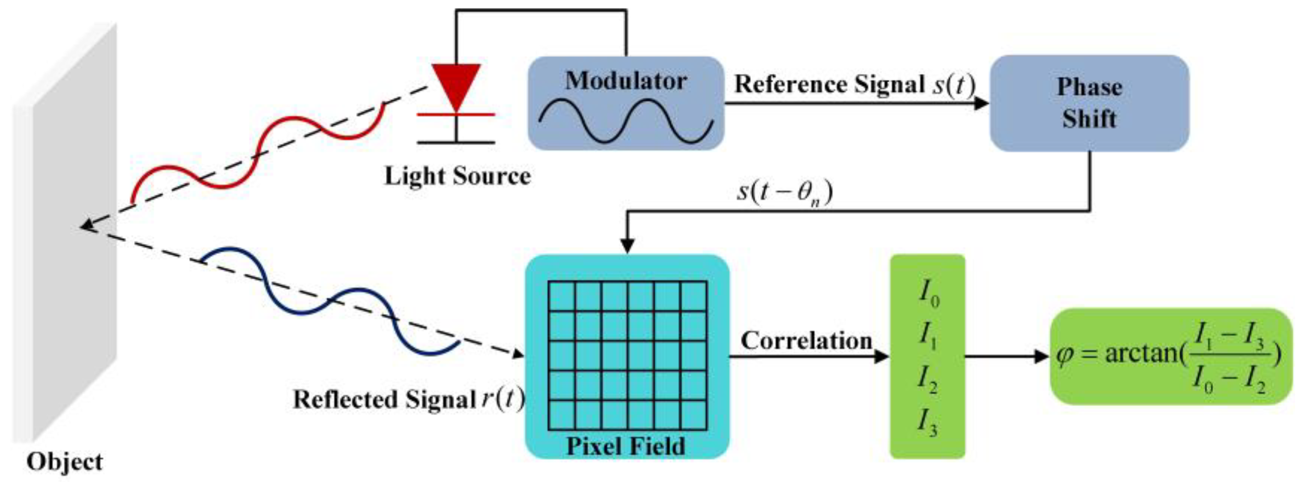
2.1. Principle of ToF Imaging Systems
2.2. Analysis of the Wiggling-Related Error
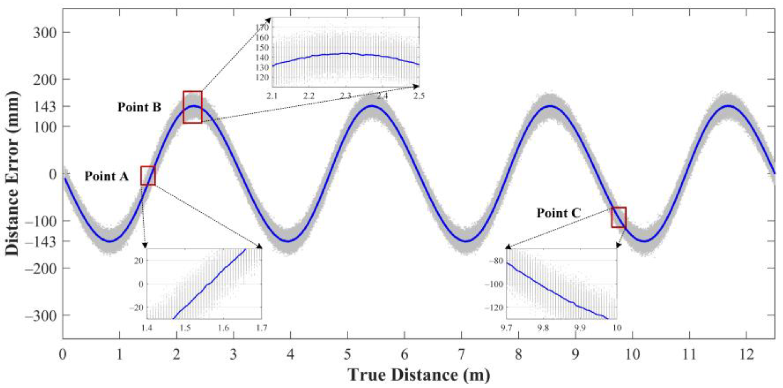
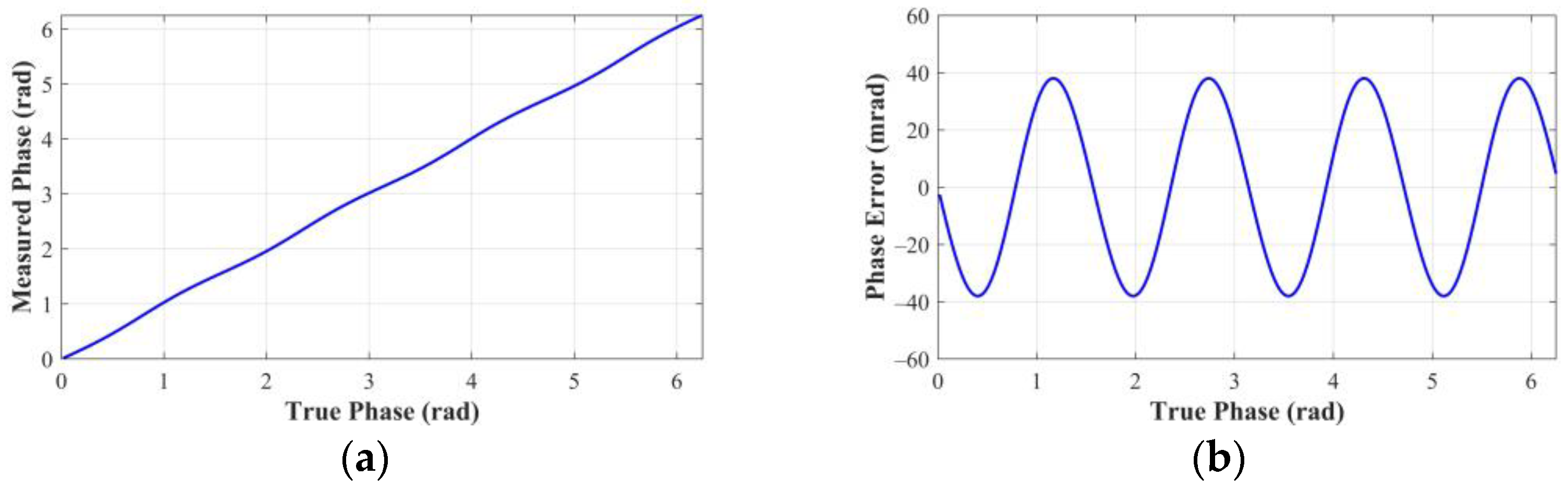
2.2.1. Wiggling Error
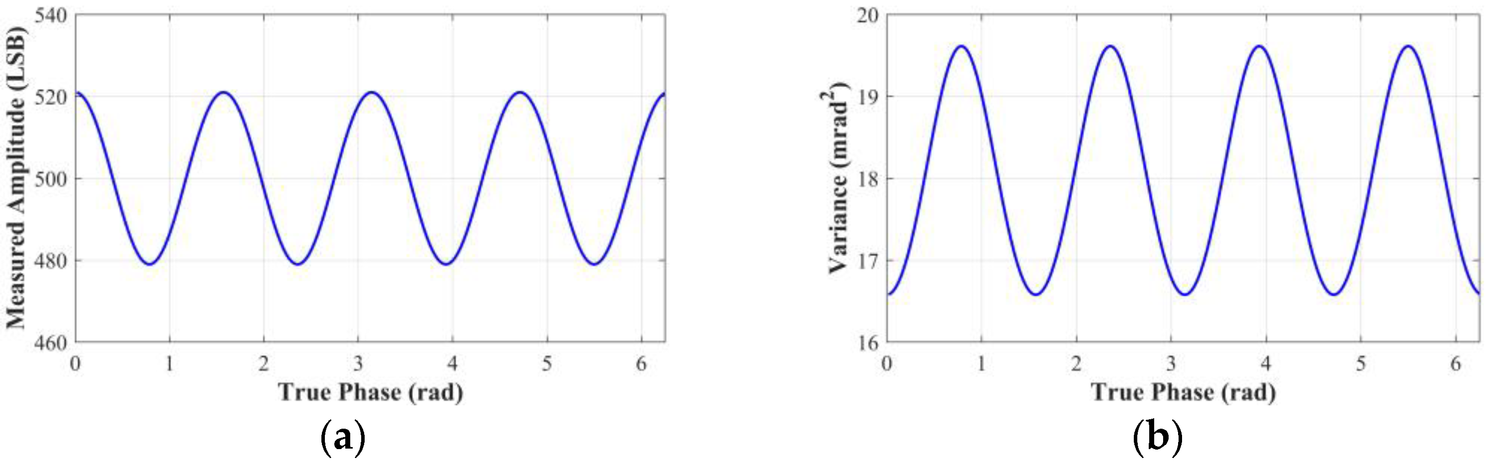
2.2.2. Wiggling Random Error
3. Methods
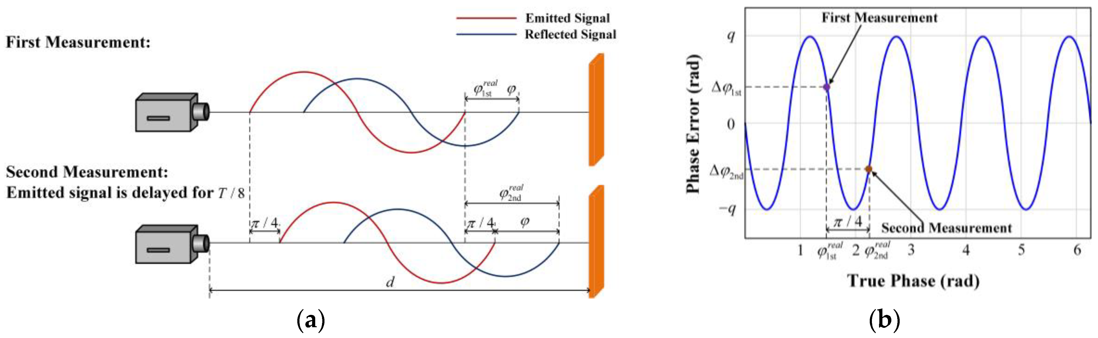
3.1. Wiggling Error Cancelation Method
- In the first measurement, calculate the measured phase without other operations;
- In the second measurement, delay the emitted signal for T/8 and calculate the measured phase ;
- Combine and to calculate the measured phased after the wiggling error cancelation:
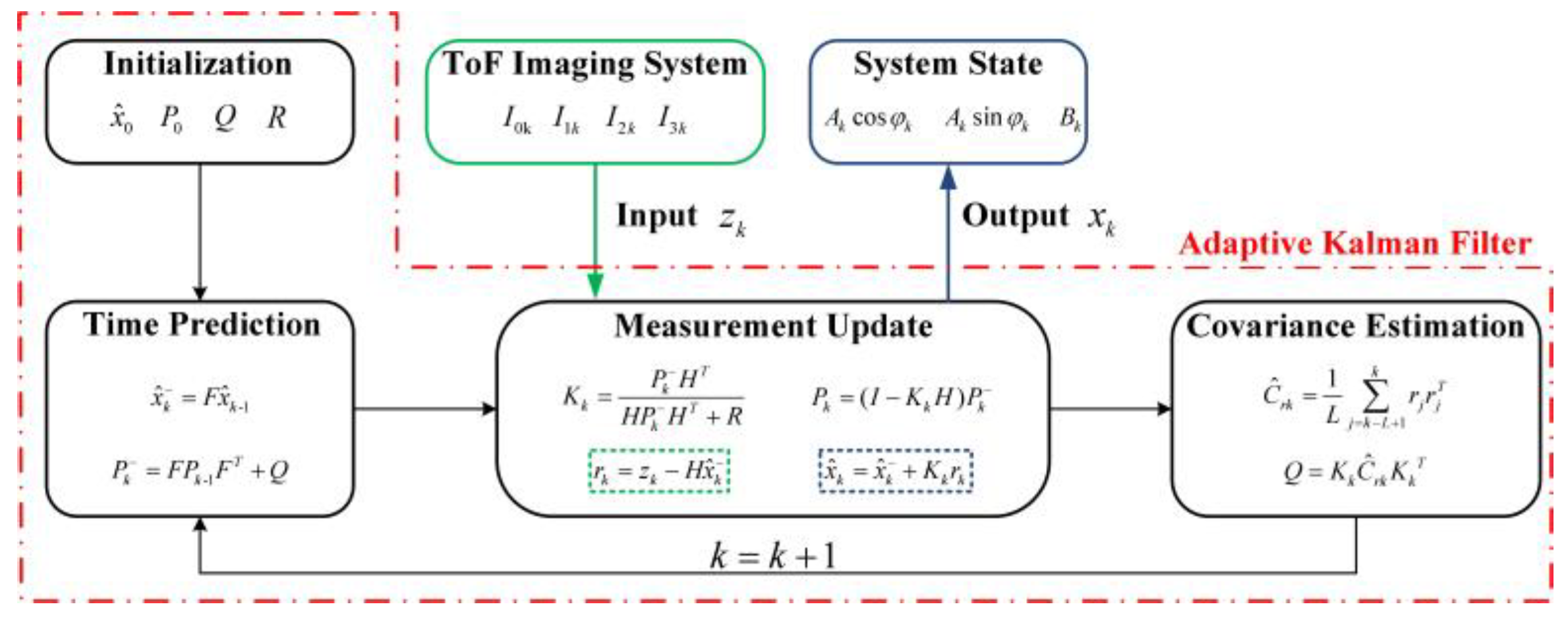
3.2. Wiggling Random Error Reduction Method
- Initialization: Initialize the state estimate , the error covariance matrix , the covariance matrix , and the covariance matrix ;
- Time Prediction: Calculate the predicted state estimate and the predicted error covariance matrix :
- Measurement Update: Calculate the Kalman gain , the updated error covariance matrix , the innovation sequence , and the updated state estimate :where is a 3 × 3 identity matrix;
- Covariance Estimation: Calculate the estimated covariance of the innovation sequence , and update the covariance matrix :where represents the length of the sliding window in the AKF.
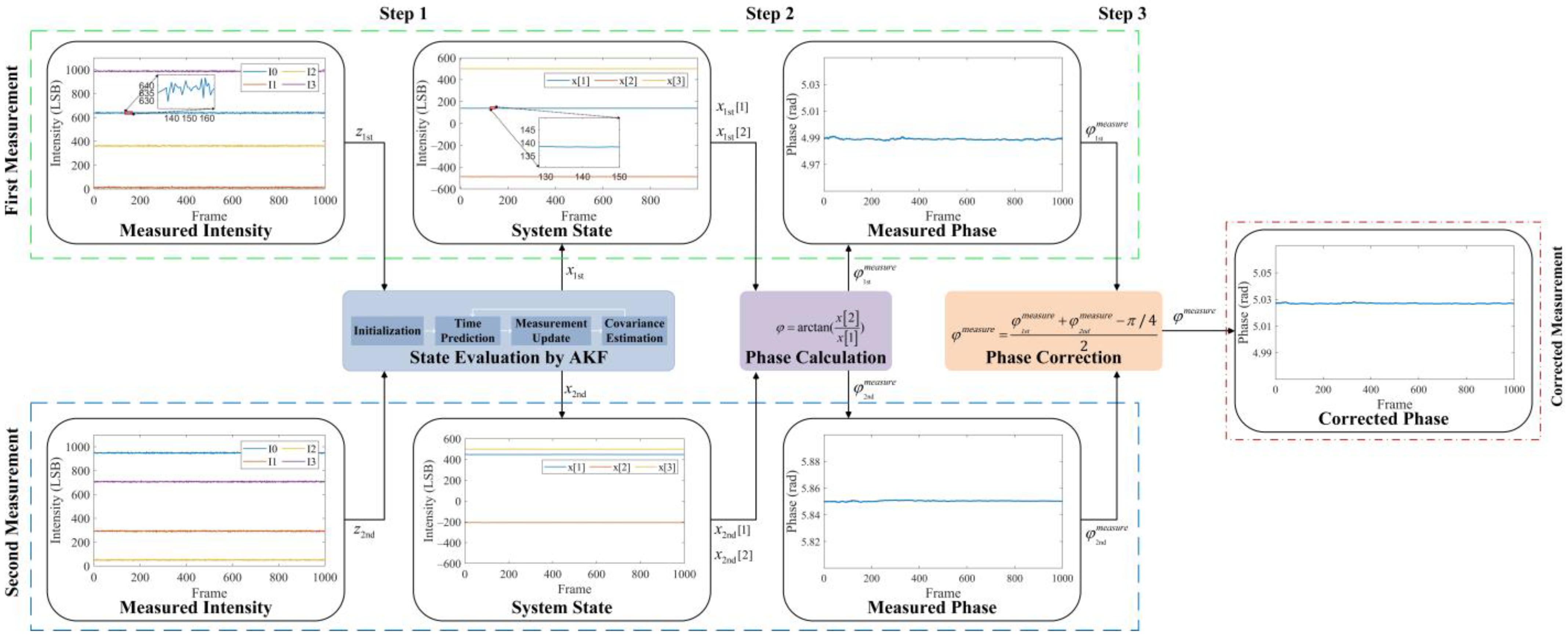
3.3. Wiggling-Related Error Correction Method
- State Evaluation: Input and into the AKF and obtain the system state vectors and ;
- Phase Calculation: Calculate the measured phases and for the two measurements. In this step, the wiggling random errors of two measurements are reduced;
- Phase Correction: Calculate the corrected phase . In this step, the wiggling error is reduced.
4. Results and Discussions
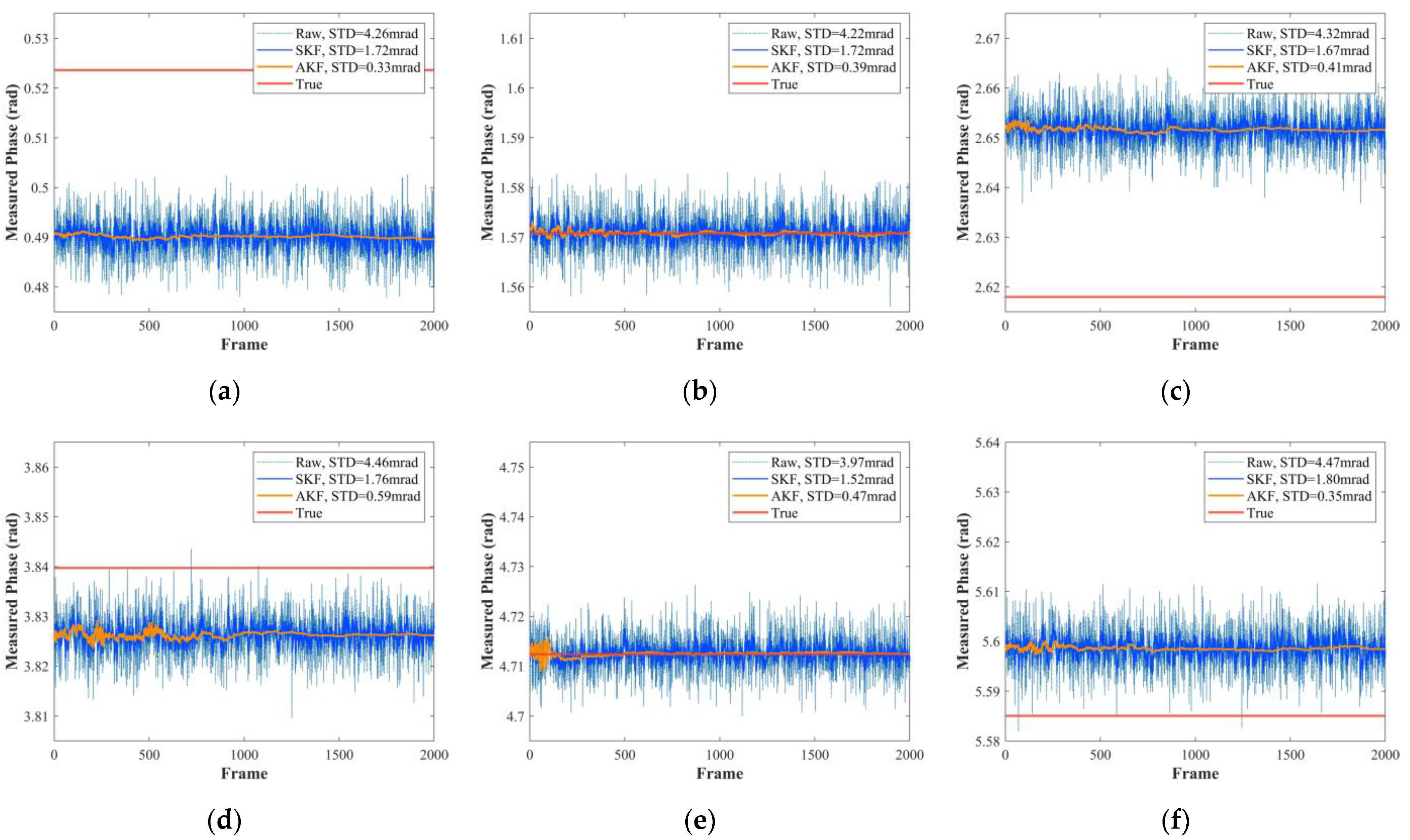
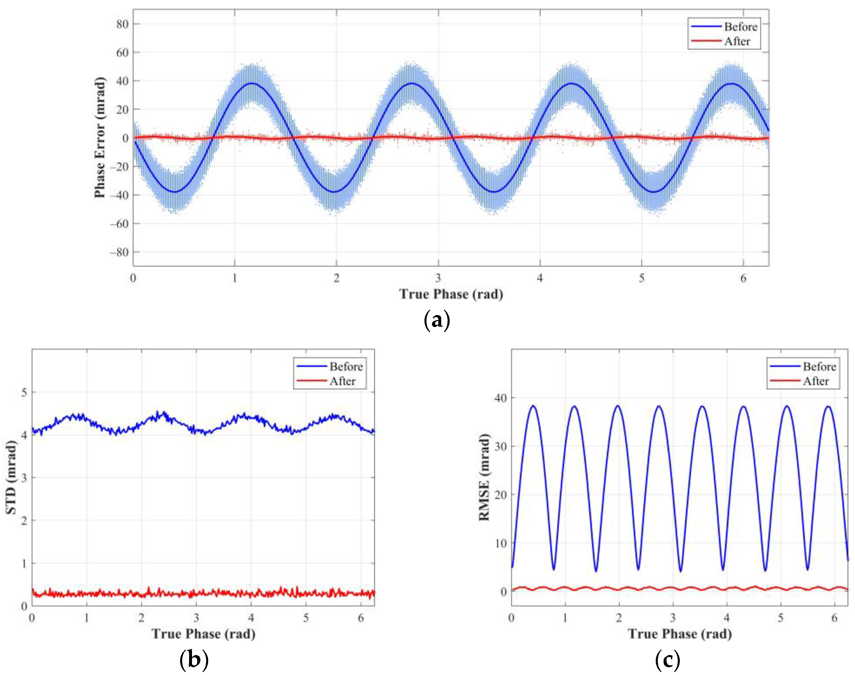
4.1. Simulation
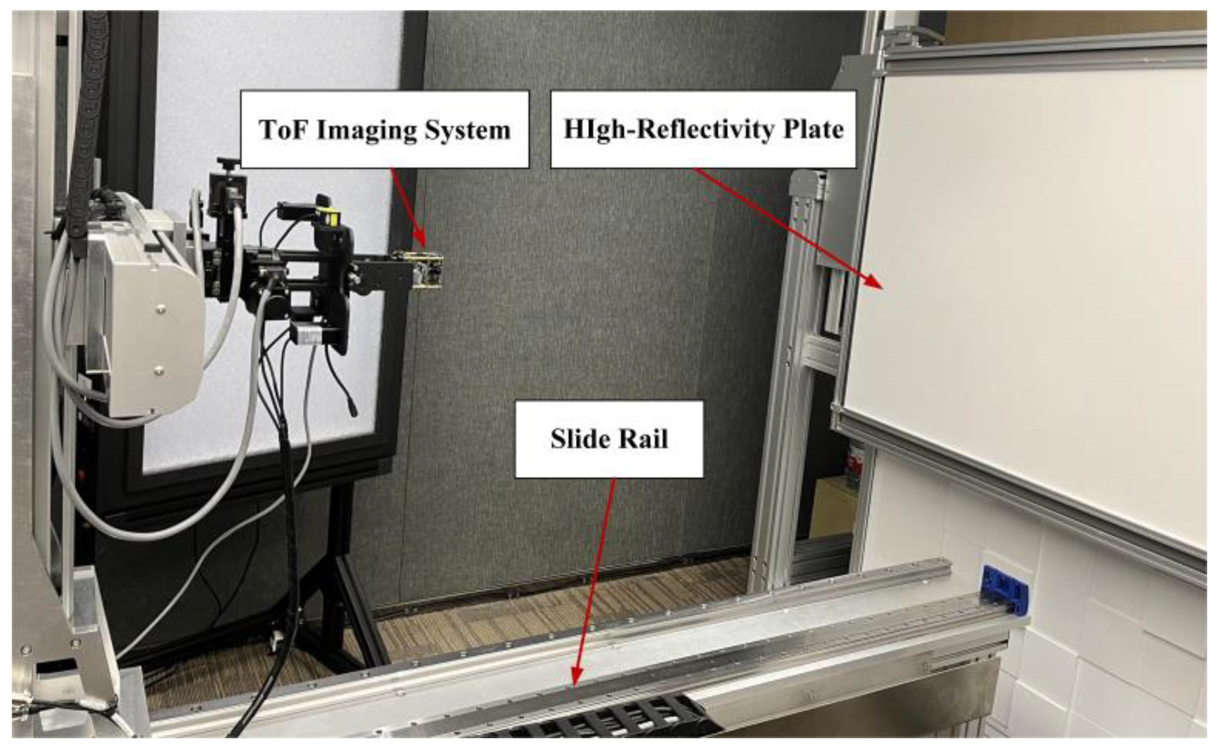
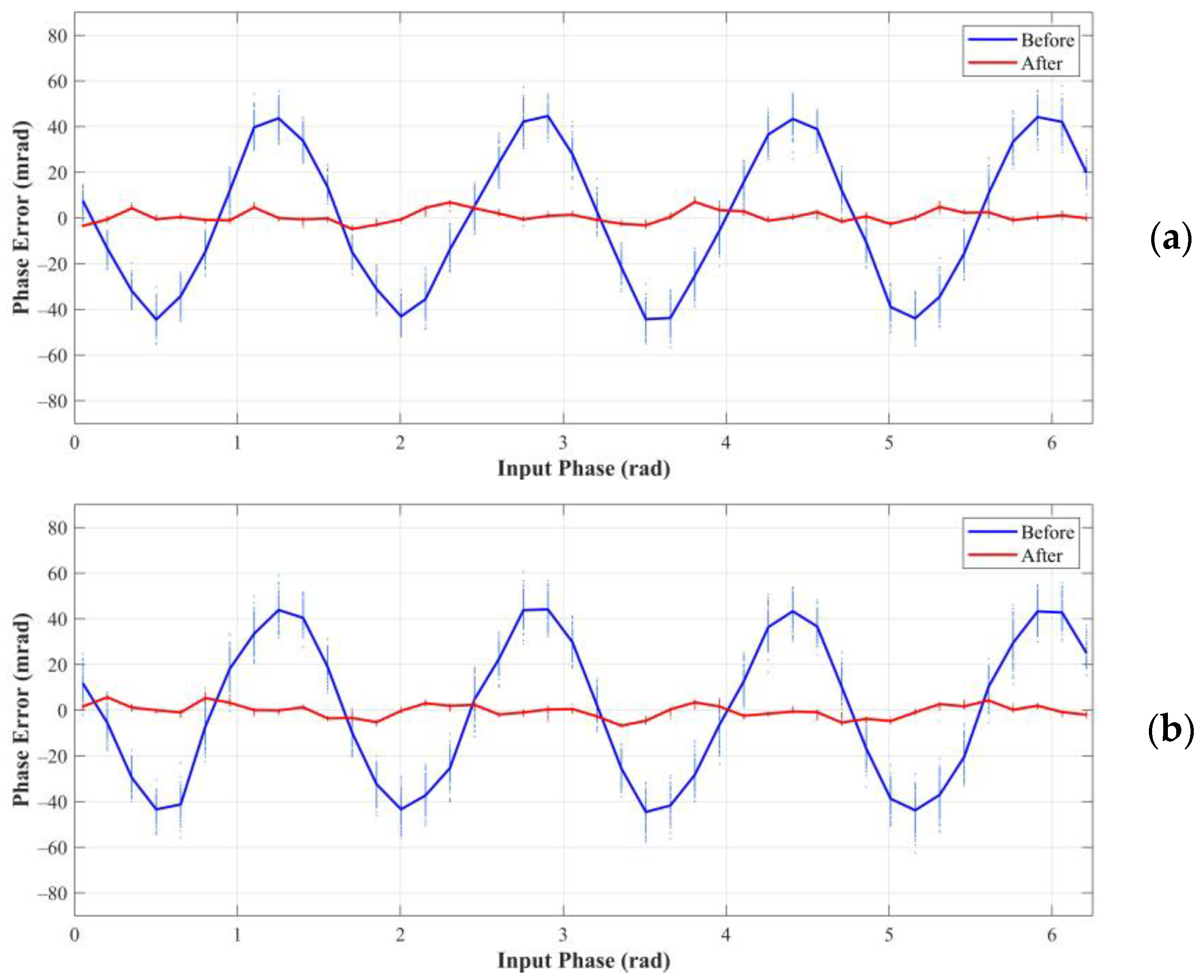
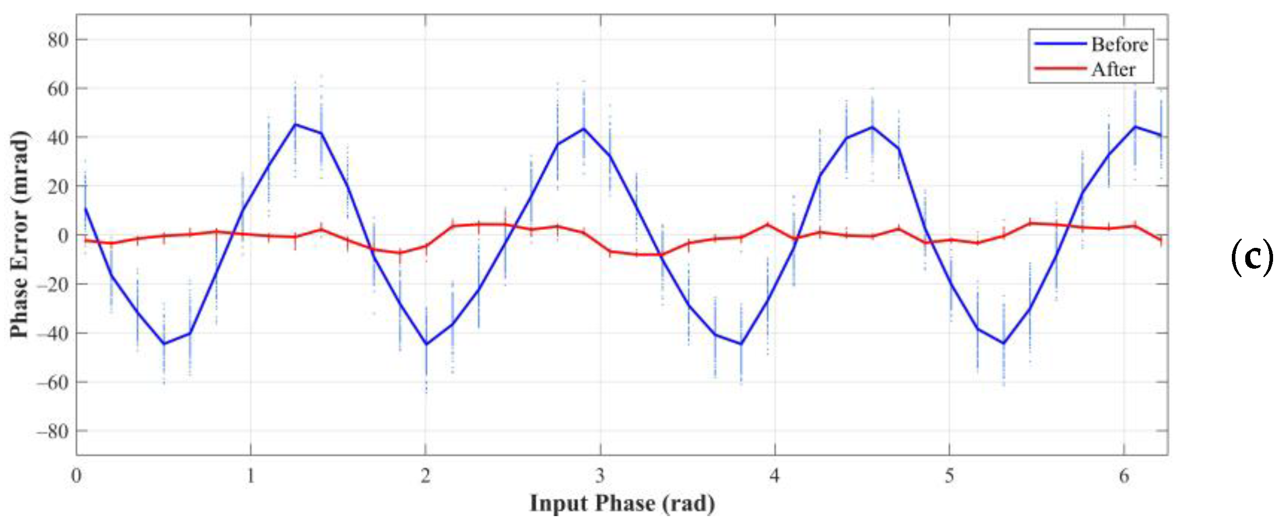
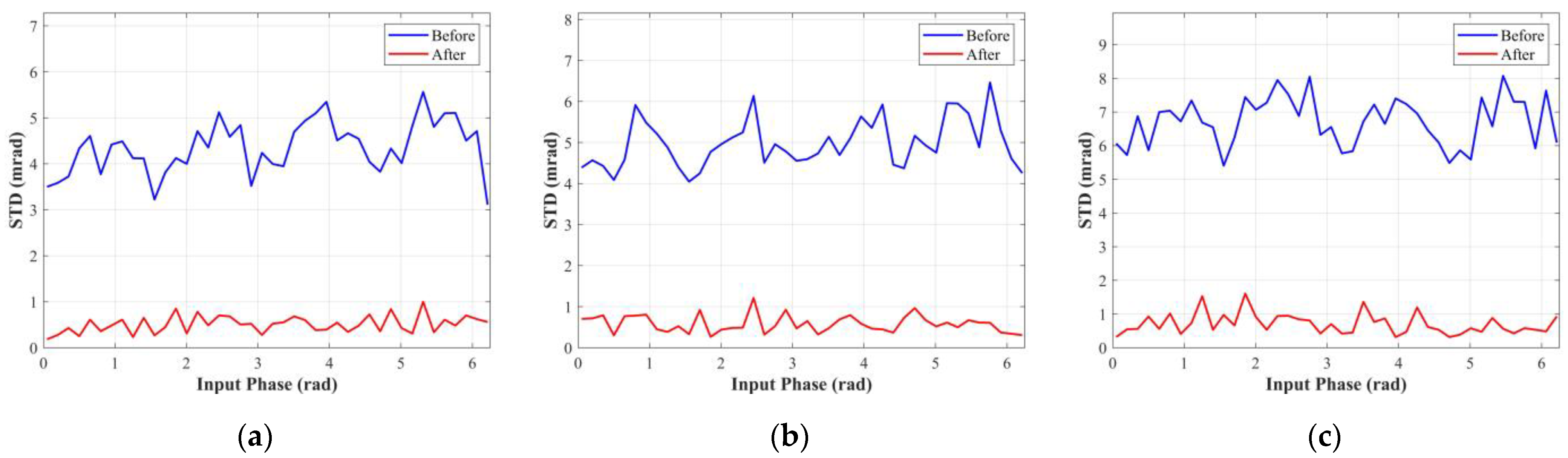
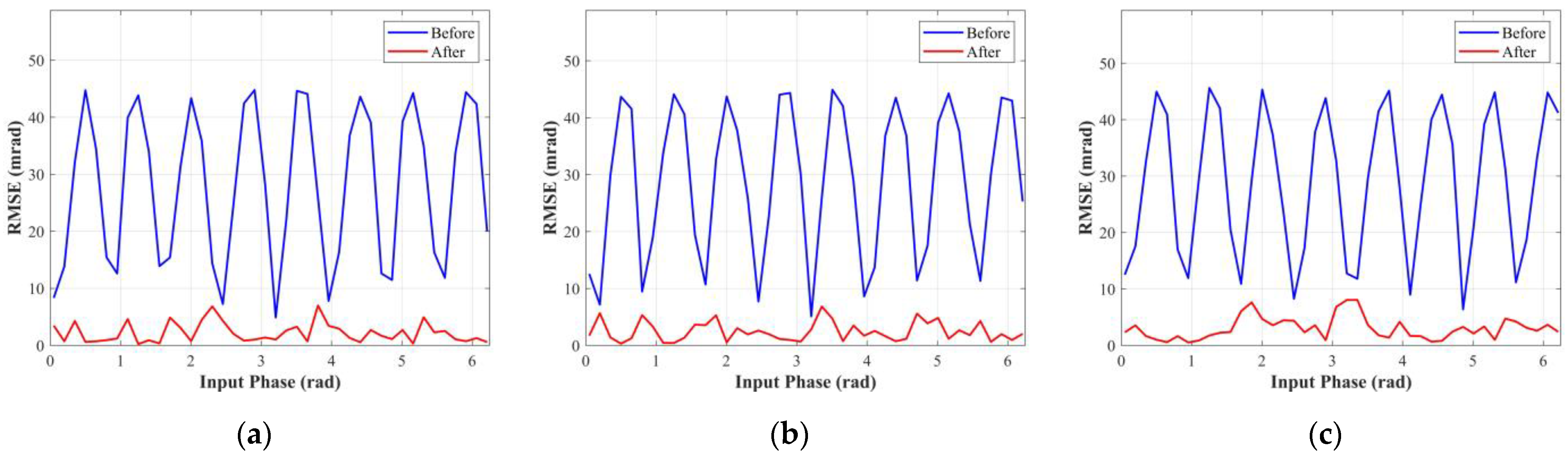
4.2. Experiment
5. Conclusions
Author Contributions
Funding
Institutional Review Board Statement
Informed Consent Statement
Data Availability Statement
Conflicts of Interest
References
- Westheimer, G. Three-dimensional displays and stereo vision. Proc. R. Soc. B-Biol. Sci. 2011, 278, 2241–2248. [Google Scholar] [CrossRef] [PubMed]
- Gong, B.X.; Wang, G.Y. Underwater Image Recovery Using Structured Light. IEEE Access 2019, 7, 77183–77189. [Google Scholar] [CrossRef]
- Foix, S.; Alenya, G.; Torras, C. Lock-in Time-of-Flight (ToF) Cameras: A Survey. IEEE Sens. J. 2011, 11, 1917–1926. [Google Scholar] [CrossRef]
- Francis, S.L.; Anavatti, S.G.; Garratt, M.; Shim, H. A ToF-camera as a 3D Vision Sensor for Autonomous Mobile Robotics. Int. J. Adv. Robot. Syst. 2015, 12, 156. [Google Scholar] [CrossRef]
- Robla, S.; Llata, J.R.; Torre-Ferrero, C.; Sarabia, E.G.; Becerra, V.; Perez-Oria, J. Visual sensor fusion for active security in robotic industrial environments. EURASIP J. Adv. Signal Process. 2014, 1, 88. [Google Scholar] [CrossRef]
- Tong, J.; Zhou, J.; Liu, L.G.; Pan, Z.G.; Yan, H. Scanning 3D Full Human Bodies Using Kinects. IEEE Trans. Vis. Comput. Graph. 2012, 18, 643–650. [Google Scholar] [CrossRef] [PubMed]
- Vazquez-Arellano, M.; Reiser, D.; Paraforos, D.S.; Garrido-Izard, M.; Burce, M.E.; Griepentrog, H.W. 3-D reconstruction of maize plants using a time-of-flight camera. Comput. Electron. Agric. 2018, 145, 235–247. [Google Scholar] [CrossRef]
- Molina, J.; Pajuelo, J.A.; Martínez, J.M. Real-time Motion-based Hand Gestures Recognition from Time-of-Flight Video. J. Signal Process. Syst. Signal Image Video Technol. 2017, 86, 17–25. [Google Scholar] [CrossRef]
- Hu, C.Z.; Zhang, B.; Xin, Y.Z.; Li, D.; Guo, Z.Q.; Xue, Z.M.; Ke, Z.G.; Geng, L. Compact Numerical Modeling of Indirect Time-of-Flight CMOS Image Sensors. IEEE Trans. Electron. Devices 2022, 69, 6897–6903. [Google Scholar] [CrossRef]
- Keel, M.S.; Jin, Y.G.; Kim, Y.; Kim, D.; Kim, Y.; Bae, M.; Chung, B.; Son, S.; Kim, H.; An, T.; et al. A VGA Indirect Time-of-Flight CMOS Image Sensor With 4-Tap 7-μm Global-Shutter Pixel and Fixed-Pattern Phase Noise Self-Compensation. IEEE J. Solid-State Circuit 2020, 55, 889–897. [Google Scholar] [CrossRef]
- Chiabrando, F.; Chiabrando, R.; Piatti, D.; Rinaudo, F. Sensors for 3D Imaging: Metric Evaluation and Calibration of a CCD/CMOS Time-of-Flight Camera. Sensors 2009, 9, 10080–10096. [Google Scholar] [CrossRef]
- Rapp, H. Experimental and Theoretical Investigation of Correlating ToF-Camera Systems. Ph.D. Thesis, University of Heidelberg, Heidelberg, Germany, 2007. [Google Scholar]
- Lindner, M.; Schiller, I.; Schiller, I.; Koch, R. Time-of-Flight sensor calibration for accurate range sensing. Comput. Vis. Image Underst. 2010, 114, 1318–1328. [Google Scholar] [CrossRef]
- Illade-Quinteiro, J.; Brea, V.M.; Lopez, P.; Cabello, D.; Domenech-Asensi, G. Distance Measurement Error in Time-of-Flight Sensors Due to Shot Noise. Sensors 2015, 15, 4624–4642. [Google Scholar] [CrossRef]
- Streeter, L.; Dorrington, A.A. Simple harmonic error cancellation in time of flight range imaging. Opt. Lett. 2015, 40, 5391–5394. [Google Scholar] [CrossRef]
- He, Y.; Chen, S.Y. Recent Advances in 3D Data Acquisition and Processing by Time-of-Flight Camera. IEEE Access 2019, 7, 12495–12510. [Google Scholar] [CrossRef]
- Mersmann, S.; Seitel, A.; Erz, M.; Jaehne, B.; Nickel, F.; Mieth, M.; Mehrabi, A.; Maier-Hein, L. Calibration of time-of-flight cameras for accurate intraoperative surface reconstruction. Med. Phys. 2013, 40, 082701. [Google Scholar] [CrossRef] [PubMed]
- Hussmann, S.; Knoll, F.; Edeler, T. Modulation Method Including Noise Model for Minimizing the Wiggling Error of TOF Cameras. IEEE Trans. Instrum. Meas. 2014, 63, 1127–1136. [Google Scholar] [CrossRef]
- Payne, A.D.; Dorrington, A.A.; Cree, M.J.; Carnegie, D.A. Improved measurement linearity and precision for AMCW time-of-flight range imaging cameras. Appl. Optics 2010, 49, 4392–4403. [Google Scholar] [CrossRef]
- Payne, A.D.; Dorrington, A.A.; Cree, M.J. Illumination waveform optimization for time-of-flight range imaging cameras. In Proceedings of the SPIE, Videometrics, Range Imaging, and Applications XI, Munich, Germany, 25–26 May 2011. [Google Scholar]
- Xuan, V.N.; Weihs, W.; Loffeld, O. Illumination, phase step optimization and improvements in simultaneous multiple frequency measurement for Time-of-Flight sensors. In Proceedings of the 2015 International Conference on 3D Imaging (IC3D 2015), Liege, Belgium, 14–15 December 2015. [Google Scholar]
- Lindner, M.; Kolb, A.; Ringbeck, T. New insights into the calibration of ToF-sensors. In Proceedings of the 2008 IEEE Computer Society Conference on Computer Vision and Pattern Recognition Workshops, Anchorage, AK, USA, 23–28 June 2008. [Google Scholar]
- Drayton, B.M.; Carnegie, D.A.; Dorrington, A.A. Phase Algorithms for Reducing Axial Motion and Linearity Error in Indirect Time of Flight Cameras. IEEE Sens. J. 2013, 13, 3386–3396. [Google Scholar] [CrossRef]
- Feigin, M.; Whyte, R.; Bhandari, A.; Dorington, A.; Raskar, R. Modeling “wiggling” as a multi-path interference problem in AMCW ToF imaging. Opt. Express 2015, 23, 19213–19225. [Google Scholar] [CrossRef]
- Lange, R. 3D Time-of-Flight Distance Measurement with Custom Solid-State Image Sensors in CMOS/CCD-Technology. Ph.D. Thesis, University of Siegen, Siegen, Germany, 2000. [Google Scholar]
- Frank, M.; Plaue, M.; Rapp, H.; Koethe, U.; Jaehne, B.; Hamprecht, F. Theoretical and experimental error analysis of continuous-wave time-of-flight range cameras. Opt. Eng. 2009, 48, 013602. [Google Scholar] [CrossRef]
- Zuo, C.; Feng, S.J.; Huang, L.; Tao, T.Y.; Yin, W.; Chen, Q.; Luan, X. Phase shifting algorithms for fringe projection profilometry: A review. Opt. Lasers Eng. 2018, 109, 23–59. [Google Scholar] [CrossRef]
- Surrel, Y. Design of algorithms for phase measurements by the use of phase stepping. Appl. Opt. 1996, 35, 51–60. [Google Scholar] [CrossRef]
- Pan, B.; Qian, K.M.; Huang, L.; Asundi, A. Phase error analysis and compensation for nonsinusoidal waveforms in phase-shifting digital fringe projection profilometry. Opt. Lett. 2009, 34, 416–418. [Google Scholar] [CrossRef]
- Schonlieb, A.; Almer, M.; Lugitsch, D.; Steger, C.; Holweg, G.; Druml, N. Coded Modulation Simulation Framework for Time-of-Flight Cameras. In Proceedings of the 2019 22nd Euromicro Conference on Digital System Design (DSD), Kallithea, Greece, 28–30 August 2019. [Google Scholar]
- Ortiz, S.; Sathiaseelan, M.A.; Cha, A. Time-of-flight camera characterization with functional modeling for synthetic scene generation. Opt. Express 2021, 29, 37661–37682. [Google Scholar] [CrossRef] [PubMed]
- Luan, X. Experimental Investigation of Photonic Mixer Device and Development of TOF 3D Ranging Systems Based on PMD Technology. Ph.D. Thesis, University of Siegen, Siegen, Germany, 2001. [Google Scholar]
- Belhedi, A.; Bartoli, A.; Bourgeois, S.; Gay-Bellile, V.; Hamrouni, K.; Sayd, P. Noise modelling in time-of-flight sensors with application to depth noise removal and uncertainty estimation in three-dimensional measurement. IET Comput. Vis. 2015, 9, 967–977. [Google Scholar] [CrossRef]
- Streeter, L. Time-of-Flight Range Image Measurement in the Presence of Transverse Motion Using the Kalman Filter. IEEE Trans. Instrum. Meas. 2018, 67, 1573–1578. [Google Scholar] [CrossRef]
- Li, M.H.; Kang, R.J.; Branson, D.T.; Dai, J.S. Model-Free Control for Continuum Robots Based on an Adaptive Kalman Filter. IEEE-ASME Trans. Mechatron. 2018, 23, 286–297. [Google Scholar] [CrossRef]
- Mohamed, A.H.; Schwarz, K.P. Adaptive Kalman Filtering for INS/GPS. J. Geodesy 1999, 73, 193–203. [Google Scholar] [CrossRef]
- Fursattel, P.; Placht, S.; Balda, M.; Schaller, C.; Hofmann, H.; Maier, A.; Riess, C. A Comparative Error Analysis of Current Time-of-Flight Sensors. IEEE Trans. Comput. Imaging 2016, 2, 27–41. [Google Scholar] [CrossRef]
- Schmidt, M. Analysis, Modeling and Dynamic Optimization of 3D Time-of-Flight Imaging Systems. Ph.D. Thesis, University of Heidelberg, Heidelberg, Germany, 2011. [Google Scholar]
- Wang, X.Q.; Song, P.; Zhang, W.Y.; Bai, Y.J.; Zheng, Z.L. A systematic non-uniformity correction method for correlation-based ToF imaging. Opt. Express 2022, 30, 1907–1924. [Google Scholar] [CrossRef] [PubMed]


| Parameters | Symbol | Value |
|---|---|---|
| The amplitude of the fundamental harmonic | 500 LSB | |
| The amplitude of the third-order harmonic | 20 LSB | |
| The amplitude of the fifth-order harmonic | 1 LSB | |
| The offset of the correlation function | 500 LSB | |
| The variance of the intensity measurement | 9 LSB2 | |
| The initial state estimate | ||
| The initial error covariance matrix | ||
| The initial covariance matrix of the process noise | ||
| The initial covariance matrix of the measurement noise | ||
| The length of the sliding window | 20 |
| Parameter | 600 μs | 400 μs | 200 μs | |||
|---|---|---|---|---|---|---|
| Before | After | Before | After | Before | After | |
| PPV (mrad) | 89.15 | 11.85 | 88.70 | 12.44 | 89.90 | 12.75 |
| (mrad) | 4.35 | 0.51 | 4.98 | 0.58 | 6.72 | 0.71 |
| (mrad) | 28.03 | 2.20 | 28.85 | 2.44 | 28.95 | 3.04 |
| Method | Harmonics Cancellation | PPV of the Phase Error (mrad) | Reduction Ratio | Implementation | |
|---|---|---|---|---|---|
| Before | After | ||||
| Streeter et al. [15] | 3rd | 70.00 | 20.00 | 71.4% | Change intensity measurement process |
| Hussmann et al. [18] | 2nd–5th | 83.78 | 11.73 | 86.0% | Add an illumination module |
| Payne et al. [20] | 3rd and 5th | 99.53 | 19.35 | 80.6% | Add an additional FPGA |
| The proposed method | 3rd and 5th | 114.50 | 14.64 | 87.2% | Add a delay measurement |
Disclaimer/Publisher’s Note: The statements, opinions and data contained in all publications are solely those of the individual author(s) and contributor(s) and not of MDPI and/or the editor(s). MDPI and/or the editor(s) disclaim responsibility for any injury to people or property resulting from any ideas, methods, instructions or products referred to in the content. |
© 2023 by the authors. Licensee MDPI, Basel, Switzerland. This article is an open access article distributed under the terms and conditions of the Creative Commons Attribution (CC BY) license (https://creativecommons.org/licenses/by/4.0/).
Share and Cite
Zheng, Z.; Song, P.; Wang, X.; Zhang, W.; Bai, Y. Wiggling-Related Error Correction Method for Indirect ToF Imaging Systems. Photonics 2023, 10, 170. https://doi.org/10.3390/photonics10020170
Zheng Z, Song P, Wang X, Zhang W, Bai Y. Wiggling-Related Error Correction Method for Indirect ToF Imaging Systems. Photonics. 2023; 10(2):170. https://doi.org/10.3390/photonics10020170
Chicago/Turabian StyleZheng, Zhaolin, Ping Song, Xuanquan Wang, Wuyang Zhang, and Yunjian Bai. 2023. "Wiggling-Related Error Correction Method for Indirect ToF Imaging Systems" Photonics 10, no. 2: 170. https://doi.org/10.3390/photonics10020170