TPDNet: Texture-Guided Phase-to-DEPTH Networks to Repair Shadow-Induced Errors for Fringe Projection Profilometry

Abstract

This paper proposes a phase-to-depth deep learning model to repair shadow-induced errors for fringe projection profilometry (FPP). The model comprises two hourglass branches that extract information from texture images and phase maps and fuses the information from the two branches by concatenation and weights. The input of the proposed model contains texture images, masks, and unwrapped phase maps, and the ground truth is the depth map from CAD models. A loss function was chosen to consider image details and structural similarity. The training data contain 1200 samples in the verified virtual FPP system. After training, we conduct experiments on the virtual and real-world scanning data, and the results support the model’s effectiveness. The mean absolute error and the root mean squared error are $1.0279$ mm and $1.1898$ mm on the validation dataset. In addition, we analyze the influence of ambient light intensity on the model’s performance. Low ambient light limits the model’s performance as the model cannot extract valid information from the completely dark shadow regions in texture images. The contribution of each branch network is also investigated. Features from the texture-dominant branch are leveraged as guidance to remedy shadow-induced errors. Information from the phase-dominant branch network makes accurate predictions for the whole object. Our model provides a good reference for repairing shadow-induced errors in the FPP system.

1. Introduction

Fringe projection profilometry (FPP) has been widely applied in many fields, such as entertainment, remote environment reconstruction, manufacturing, medicine, and biology, due to its high accuracy and high-speed [1,2]. A typical FPP system comprises a projector for fringe pattern projection and a camera for image acquisition. The projector projects fringe pattern images onto the object surface, and the camera captures the fringe pattern images encoded by the object surface from a different perspective. Due to the triangulation of the projector, the camera, and the object, the light emitted from the projector is blocked by the adjacent surface of the object, leaving shadows in the captured images. As shown in Figure 1, shadows exist in the acquired fringe images, causing errors in the same areas of the wrapped phase map and unwrapped phase map. As the phase information of shadow-covered areas is lost, 3D reconstructed geometry in shadow areas cannot be obtained based on phase maps, which reduces the accuracy of FPP methods.

The simplest idea to remove shadow-induced errors is to avoid shadow generation in fringe pattern images. As shadow errors are due to triangulation of the camera, the projector, and the object, some researchers proposed uniaxial techniques [3,4,5] to make the projector and the camera share the same optical axis and have the same region of projection and imaging. In uniaxial techniques, the retrieved 3D geometry is based on the relationship between depth and phase (or intensity or level of defocus), and beam splitters are commonly used. The projector and camera’s optical axis and the beam splitter must be fixed at a specific angle to ensure a coaxial configuration, which increases system complexity and limits its application. Another method to reduce shadow errors is to use multiple devices. In the work of Skydan et al. [6], three video projectors were set up at different angles and exclusively projected three different colored lighting patterns. Shadow areas that were not illuminated by one projector would be covered by another projector with different colored lighting patterns. And this method combined information from these two colored lighting patterns to reduce shadows. However, potential errors were brought as extra masks had to be produced to separate the valid areas and shadows. Meanwhile, the system complexity and cost increase with the number of projectors. Weinmann et al. [7] proposed a super-resolution structured light system with multiple cameras and projectors to cover the full shape of objects with super-resolution. Though the proposed system could obtain full 3D reconstruction with high accuracy, complicated post-processing was needed. For the above methods, the hardware cost is higher than a typical FPP system with one projector and one camera, and extra post-processing or pre-processing cannot be avoided.

In addition to avoiding the generation of shadow artifacts in fringe pattern images, researchers have also attempted to eliminate shadow-induced errors during the phase retrieval stage. Various frameworks and methods have been employed to identify and eliminate invalid data points in the phase maps, including those presented in prior works [8,9,10]. Although these methods do not introduce additional errors, they can create voids in the final 3D reconstruction results. To address this issue, Zhang [11] utilized phase monotonicity to detect and remove erroneous unwrapped points in low-illuminated regions of an object’s surface, and filled the resulting voids in the phase map. Similarly, Chen et al. [12] employed the standard deviation of the least-squares fitting to detect and remove invalid phase points, followed by recalculating the phase values using two-dimensional linear interpolation. However, interpolation or similar techniques are not particularly accurate in estimating lost phase information, particularly in objects with abrupt surface profile changes. In contrast to interpolation methods, Sun et al. [13] proposed a discriminative approach, which classified shadows into valid and invalid shadow areas, and then utilized different smoothing methods to reduce shadow-induced errors. Although this method was effective against large-scale shadows, its performance was hindered by incorrect shadow classification, and its efficacy decreased when the unwrapped phase map was obtained using the spatial phase unwrapping technique.

Over the past few years, tremendous research has been developed in computer vision based on deep learning, and a series of remarkable achievements have been made, which also attracted researchers’ interests in applying deep learning to three main steps of optical metrology, including pre-processing, phase analysis, and post-processing [14]. For example, Yan et al. [15] proposed a deep convolutional neural network to reduce the noise of the fringe pattern images, which obtained high-quality fringe pattern images at the pre-processing stage. In addition, deep learning is also leveraged to solve the tasks of phase analysis, including phase demodulation [16,17,18], phase unwrapping [19,20], phase map denoising [21,22], and so on. Meanwhile, Li et al. [23] used a network to make an accurate phase-to-height mapping. Except for networks targeted at one or two stages of image processing in optical metrology, end-to-end neural networks were developed to directly convert fringe pattern images to depth maps or even 3D shapes [24,25,26].

Repairing shadow-induced holes in phase maps can be regarded as a type of image completion problem, which has been the subject of much research [27]. But to our knowledge, few neural networks have been developed to repair the shadow-induced errors in the FPP system, likely due to the difficulty of generating sufficient training data. However, FPP systems can be virtualized through 3D graphics to rapidly generate training data [26], laying the foundation for repairing shadow-induced errors based on deep learning. Utilizing a virtual system built with the graphic software Blender [28], Wang et al. [29] proposed a deep learning method to detect and repair shadow-induced errors. Their method can be conducted by only one fringe image, which makes it flexible to many FPP systems. But the effectiveness of their model is influenced by the reliability of shadow detection. Thus, methods that can avoid shadow detection and segmentation are worth trying.

To complement these methods, we propose a phase-to-depth deep learning model to repair shadow-induced errors. The proposed model contains two hourglass branch networks: a texture-dominant branch network and a phase-dominant branch network. The two combined branch networks extract information from texture images and phase maps, predict depth maps, and repair errors caused by shadows. The proposed model fuses information from texture images and phase maps in the following locations:

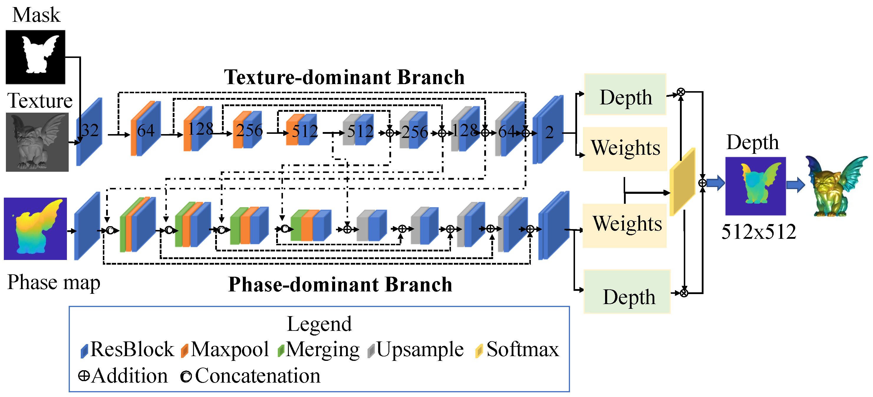
• Each layer in the encoder stage of the phase-dominant branch is fused with a layer from the decoder stage of the other branch via concatenation and addition
• At the end of the decoder stage, depth maps from two branches are fused by multiplying the respective weights.

To generate enough training data, we build and evaluate the virtual system of a real-world FPP system based on computer graphics. After training the proposed model on the virtual scanning data, the mean absolute error (MAE) and root mean squared error (RMSE) are $1.0279$ mm and $1.1898$ mm, respectively. Experimental results on the real-world scanning data support the model’s effectiveness. In addition, we analyzed the influence of ambient light on prediction and found that low ambient light decreases the performance of our model as valid information in texture images decreases. And properly increasing the ambient light will improve the performance of our model. We also tested the functions of the texture-dominant branch and phase-dominant branch. The results show that information from texture images contributes to remedying the holes in 3D geometry caused by shadows, and the phase-dominant branch network makes accurate predictions for the major object geometries. Our code will be available in https://github.com/JiaqiongLi/TPDNet.

2. Principles

This section will introduce the theoretical foundations of a real-world FPP system and the corresponding virtual FPP system for generating training data.

2.1. FPP Model

We adopted the three-step phase-shifting algorithm [30] to analyze fringe images, and fringe images can be described as

$$\begin{array}{c}\hfill I_k(x,y)=I^{\prime }(x,y)+I^{″}(x,y)cos\left[\varphi (x,y)+{\delta }_k\right],\end{array}$$

(1)

$$\begin{array}{c}\hfill {\delta }_k=\frac{2k\pi }{N};N=3,k=1,2,3,\end{array}$$

(2)

where $I_k(x,y)$ denotes the image intensity at pixel $(x,y)$ for the kth fringe image, and $I^{\prime }(x,y)$ and $I^{″}(x,y)$ presents the average intensity and the intensity modulation, respectively. In our work, we treat the gray images with average intensity as texture images and input them into the proposed model. Phase $\varphi (x,y)$ can be calculated by,

$$\varphi (x,y)={tan}^{-1}\left[\frac{\sqrt{3}(I_1-I_3)}{2I_2-I_1-I_3}\right].$$

(3)

Given the discontinuity of the arctangent function, phase $\varphi (x,y)$ ranges in $[-\pi /2,\pi /2)$, which is called the wrapped phase. The absolute phase (unwrapped phase) can be obtained by

$$\Phi (x,y)=\varphi (x,y)+2\pi k(x,y).$$

(4)

Here, $\Phi (x,y)$ denotes the unwrapped absolute phase without phase jumps, and $k(x,y)$ is the fringe order. To remove the discontinuity in wrapped phase maps, we encoded the fringe order $k(x,y)$ by projecting additional binary images using a gray-coding technique [31]. The unwrapped phase maps are also part of the input for the proposed model.

2.2. Virtual FPP Model

As deep learning is a data-driven method and generating a large training dataset in a real-world FPP system is quite expensive, we replace the real-world FPP system with its virtual system for an easier generation of training data. Based on computer graphics and the open-source 3D software Blender [28], we utilized the same virtual FPP system proposed by Zheng et al. [26]. We fixed the virtual camera at the origin point to simplify the system and adopted a spotlight to mimic a real projector. The power of the spotlight is set to 30 W, and the spot size was ${180}^{\circ }$. The resolutions of the virtual camera and the virtual projector are $514\times 544$ and $912\times 1140$, respectively. The focal length of the virtual camera was $12.03$ mm, and (Shift X, Shift Y) was $(0.018,-0.021)$.

Table 1. Parameters of the virtual FPP system.

Parameters	Virtual Camera	Virtual Projector (Spot Light)
Extrinsic matrix Location	$(0,0,0)$	(0.0227 m, 0.0885 m, −0.1692 m)
Rotation	$(0^{\circ },0^{\circ },{180}^{\circ })$	$(-14.{07}^{\circ },0.{46}^{\circ },1.{44}^{\circ })$
Scale	$(1.0,1.0,1.0)$	$(0.2,0.2,1.0)$

presents other parameters of the virtual camera and the virtual projector. Ambient light intensity and exposure were set to ensure that no underexposure or overexposure is present on the model in any captured fringe images. (The effects of ambient light intensity on the model’s performance are discussed in Section 5.1).

To verify the established virtual FPP system, we compared the scanning results of the real-world FPP system and its corresponding virtual system. Utilizing the iterative closest point (ICP) algorithm and K-nearest neighbor (KNN) search [32] to make point-to-point registration of the two scanning results, the average and root-mean-square of the 3D Euclidean differences are $0.083$ mm and $0.088$ mm. Based on the similarity of the scanning results from the virtual FPP system and the real-world FPP system, the captured images from the virtual FPP system can be utilized as training data.

3. Proposed Model

In this work, we propose an hourglass deep learning model to remove shadow-induced errors and produce depth map predictions with texture images and phase maps, and combine the structural similarity index and a Laplacian pyramid loss as the loss function to optimize the training process.

3.1. Network Architecture

Inspired by the work of Hu et al. [33], we propose a model with a texture-dominant branch and a phase-dominant branch to produce depth map predictions and then fuse depth predictions from two branches by multiplying their weight maps. The network architecture is illustrated in Figure 2.

The texture-dominant branch is similar to a typical Unet [34], which is a symmetric encoder-decoder network with skip connections to produce depth map predictions and offer guidance to the phase-dominant branch. The difference is that we used the ResBlock [35] rather than the normal 2D-convolution layer as the backbone. The downsample layer contains a maxpool layer and a ResBlock layer. The upsample layer is similar to the downsample layer, which replaces the maxpool layer with a ConvTranspose2d layer. Finally, the two-channel output layer in the texture-dominant branch is split into a depth map and a weight map, which will be utilized for depth map fusion.

The phase-dominant branch also has a symmetric encoder-decoder network with skip connections, which is similar to the texture-dominant branch. The only difference is that the phase-dominant branch fuses the feature from the texture-dominant branch at the encoder stage by concatenation and a merging layer. The merging layer is composed of two 2D-convolution layers followed by a batch normalization layer and a ReLU activation. Thus, the lost phase information in the phase map can be recovered through features from the texture-dominant branch.

The depth maps from the two branches are fused using the method proposed by Gansbeke et al. [36]. Both branches produce a weight map, and the weight maps are rescaled in the range of $\left(0,1\right)$ through a softmax layer. The weight map of each branch multiplies its corresponding depth map to get the weighted depth map. And then, the weighted depth maps are added together to get the final output. Higher values in weight maps mean the corresponding depth map contributes more to the final prediction. Ideally, the model would place a higher weight on the phase-dominant branch in areas where this data is available (in areas illuminated by the projector), and the texture-dominant branch where those data are unavailable, i.e., in shadow areas. This behavior would enable the model to fill the holes caused by shadows and make accurate predictions for non-shadow regions simultaneously. The effectiveness of fusion is supported by the results in Section 4.3, and we discuss the effects of the two branches in Section 5.2.

3.2. Loss Function

One of the most commonly used loss functions in computer vision is the mean absolute error ($l_1$ loss) or the mean square error ($l_2$ loss). However, the limitations of $l_2$ loss and $l_1$ loss are obvious. $l_2$ loss assumes that noise is independent of the local characteristics of the image, and the residuals between predictions and true values follow a Gaussian distribution [37]. And $l_1$ loss assumes that the residuals follow the Laplace distribution. These assumptions are not valid in the current situation, as shadow-induced errors are related to local information of phase maps. Furthermore, both $l_1$ loss and $l_2$ loss are the metrics for evaluating average errors, which blur the edges of prediction images. Considering these limitations, our loss function contains two parts: the structural similarity index (SSIM) and the Laplacian pyramid loss. SSIM was first introduced by Wang et al. [38], which is a metric to compare the differences between two images from luminance, contrast, and structure, and it can be described as

$$SSIM(x,y)={\displaystyle \frac{(2{\mu }_x{\mu }_y+C_1)(2{\sigma }_{xy}+C_2)}{({\mu }_x^2+{\mu }_y^2+C_1)({\sigma }_x^2+{\sigma }_y^2+C_2)}}.$$

(5)

In Equation (5), ${\mu }_x$ and ${\mu }_y$ defines the mean intensity of image x and image y, ${\sigma }_x$ and ${\sigma }_y$ are the standard deviations, ${\sigma }_{xy}$ is the corresponding covariance, and $C_1$ and $C_2$ are two constants. SSIM ranges from 0 to 1. When a predicted image is more similar to the ground truth, SSIM value will be closer to 1. Thus, SSIM loss can be written as

$$L_{SSIM}=1-SSIM(P,GT),$$

(6)

where P is the prediction image and $GT$ is the ground truth. As SSIM loss focuses on the overall similarity based on the human visual system, we still need an extra metric to evaluate the details at the edges. The Laplacian pyramid ($La{p}_1$) loss [39] can describe finer details, and it is mathematically expressed as

$$La{p}_1(x,y)=\sum _{j=0}^2{2}^{2j}{\parallel L^j\left(x\right)-L^j\left(y\right)\parallel }_1,$$

(7)

where $L^j\left(x\right)$ defines the j-th level of the Laplacian pyramid representation of image x. We combine SSIM loss and Laplacian pyramid loss to evaluate prediction from the overall structural similarity and details at the edges. The loss function for the predicted depth map is

$$L={\lambda }_1{L}_{SSIM}+{\lambda }_{2}La{p}_1,$$

(8)

where ${\lambda }_1$ and ${\lambda }_2$ are hyper-parameters, given as 100 and 10 empirically in the following experiments. When training the model, depth maps from the two branches and the final predicted depth map are all considered. Thus, the training loss is

$$L_{training}=k_1{L}_{out}+k_2{L}_T+k_3{L}_P,$$

(9)

where $L_{out}$ is the loss between the ground truth and the output depth map, $L_T$ is the loss between the ground truth and the depth map from the texture-dominant branch, and $L_P$ is the loss between the ground truth and the depth map from the phase-dominant branch. Here, $k_1$, $k_2$, and $k_3$ are constants, empirically given as 1, 0.1, and 0.1.

4. Experiments

In this section, we first introduce the process to generate the training data in the verified virtual FPP system, followed by the training setup for the proposed model. Then, we implement experiments on virtual scanning data and real-world scanning data to validate the effectiveness of our model.

4.1. Dataset Preparation

Before scanning objects in the virtual FPP system, we collected 48 CAD models from public CAD model resources, including Thingi10K [40] and Free3D [41], mostly animals and statues. Based on the bounding box of an object and the focal length and resolution of the virtual camera, we calculate the coordinates of the object’s centroid and dimensions. Then the object is imported into the virtual system and positioned to fit the virtual camera’s field of view. To augment the dataset, we rotate each CAD model around the y-axis five times with ${72}^{\circ }$ each time and then do the same thing around the z-axis. Thus, we scan each CAD model from 25 different perspectives, producing 1200 3D scenes. For each 3D scene, three phase-shifting fringe patterns and six gray code images are projected on the object and captured by the virtual camera as shown in Figure 3a–i. In addition, we directly export a depth map from the virtual system as illustrated in Figure 3n, which represents the distance between the plane ($Z=0$) and the object’s surface. (Note that depth map is different from the height map of the object.) As nine images and one depth map are required for each 3D scene, $9\times 1200+1200=$ 12,000 images need to be rendered in total, which is computationally expensive for a personal computer. Therefore, we utilize a workstation with an Intel Xeon processor and eight Quadro RTX 5000 graphics cards to render images in parallel.

After obtaining the fringe images and gray code images, we obtain the corresponding texture images, wrapped phase maps, and unwrapped phase maps, based on the method mentioned in Section 2.1, which are presented in Figure 3j–l. In the wrapped phase map, the shadow caused by occlusion from the surrounding protrusion surface makes part of the phase information invalid and brings plenty of noise. By setting the light intensity threshold and modulation, we filter out noise and invalid phase points and leave holes in the unwrapped phase map. Surfaces where the fringe patterns were occluded are still visible in the texture image, so we combine the texture image and unwrapped phase map as input data and the depth map as the ground truth to train the model. By setting a suitable depth threshold, we generate the mask (Figure 3m) to remove unnecessary pixels in the texture image. Note that the related shadow areas are kept in texture images as masks are obtained by the depth threshold, not the light intensity threshold. Additionally, all the input images are cropped to $512\times 512$ before being imported into the proposed model.

4.2. Training

This subsection describes the setup for the model training process. We train the model on a workstation with an Intel Xeon processor, 128 GB RAM, and a Quadro RTX 5000 graphics card using the PyTorch library [42]. The training data (1200 data samples) from the virtual FPP system are split into 90% and 10% as a training dataset and validation dataset, respectively. The batch size is six, and the maximum epoch is 1200. We use the SGD optimizer [43] with $lr=0.0003, momentum=0.9$ and $weightdecay=0.0001$. We reduce the learning rate using the scheduler class ReduceLROnPlateau in PyTorch, and the related hyper-parameters are $mode=min, factor=0.9, patience=2, threshold=0.01, min\_lr=1\times {10}^{-6}$.

4.3. Results with Data from the Virtual System

We train and evaluate our model after setting up hyper-parameters. The mean absolute error (MAE) and root mean squared error (RMSE) are $1.0279$ mm and $1.1898$ mm for the validation dataset with 120 data samples. The results of one object are shown in Figure 4. Shadow-induced errors cause part of the phase information to be lost, and related 3D geometry cannot be retrieved directly from the phase map as presented in Figure 4d. Specifically, the whole left wing of the object is lost, and there is an abrupt depth change between the lost wing and its surroundings. The predicted depth map and retrieved 3D geometries are presented in Figure 4h,f, where the model repairs the lost part of the object. Besides, the predicted result contains the details presented in the ground truth. The rear wing of this gargoyle model represents a worst-case scenario, where the fringes have been occluded and there is an abrupt change in the depth map between this feature and the rest of the 3D model. These combined factors increase the overall RMSE for this object above the average for the validation set, at $2.6485$ mm.

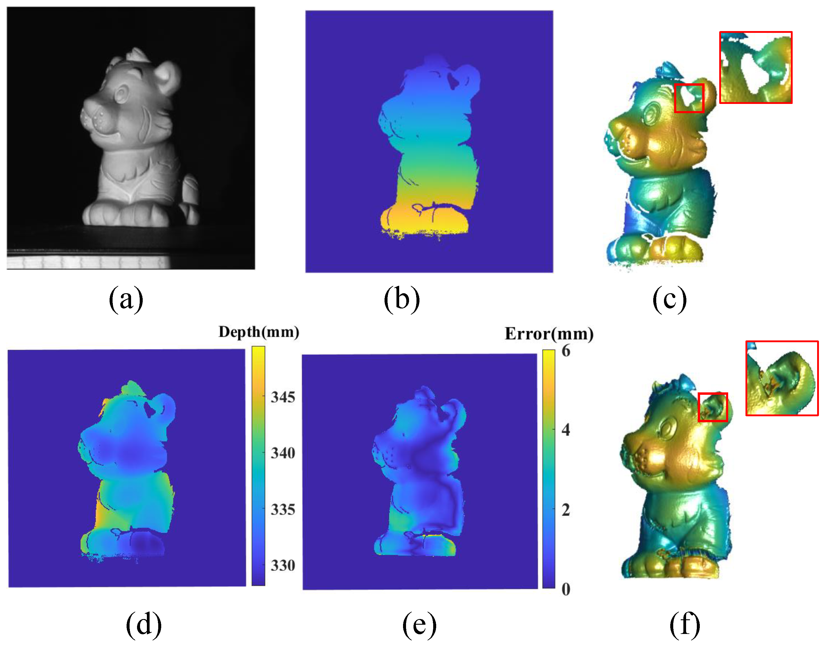
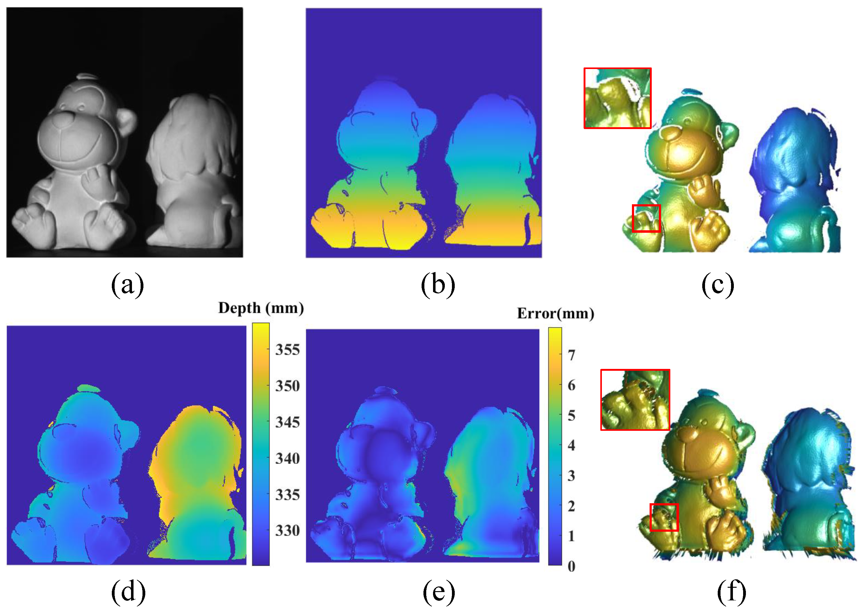
4.4. Results with Data from the Real-World System

We deployed the pre-trained model to the real-world scanning data to test the model’s effectiveness, i.e., that the model can remedy the shadow-induced errors and make good predictions for the non-shadow regions. We first scanned a single object which did not appear in the training data. The texture image and unwrapped phase map were generated as illustrated in Figure 5a,b. We manually labeled the texture image to get the mask. Importing the texture image, mask, and phase map into the pre-trained model, we obtained the predicted depth map as well as the 3D geometry as presented in Figure 5f. For the non-shadow covered region, we calculated the absolute error map as shown in Figure 5e by comparing the absolute difference between the predicted depth map and the depth map from FPP, and RMSE for the non-shadow covered region was $1.5031$ mm. All holes on the predicted 3D geometry were filled except for a minor discontinuity that occurred in the highlighted region. We assume that the low light intensity in the texture image’s shadow areas causes the model to not extract enough valid information to fill the holes, and a detailed investigation in this regard is conducted in Section 5.1.

Similarly, we scanned the two separate objects, as shown in Figure 6a. The two-object scene was not included in the training data. We also recovered the 3D geometry for the two objects, as presented in Figure 6f. The RMSE of these two objects in the non-shadow region was $2.3579$ mm, which kept the same level of accuracy as the prediction for a single object. Therefore, results from real-world experiments validate the effectiveness of our model.

5. Discussion

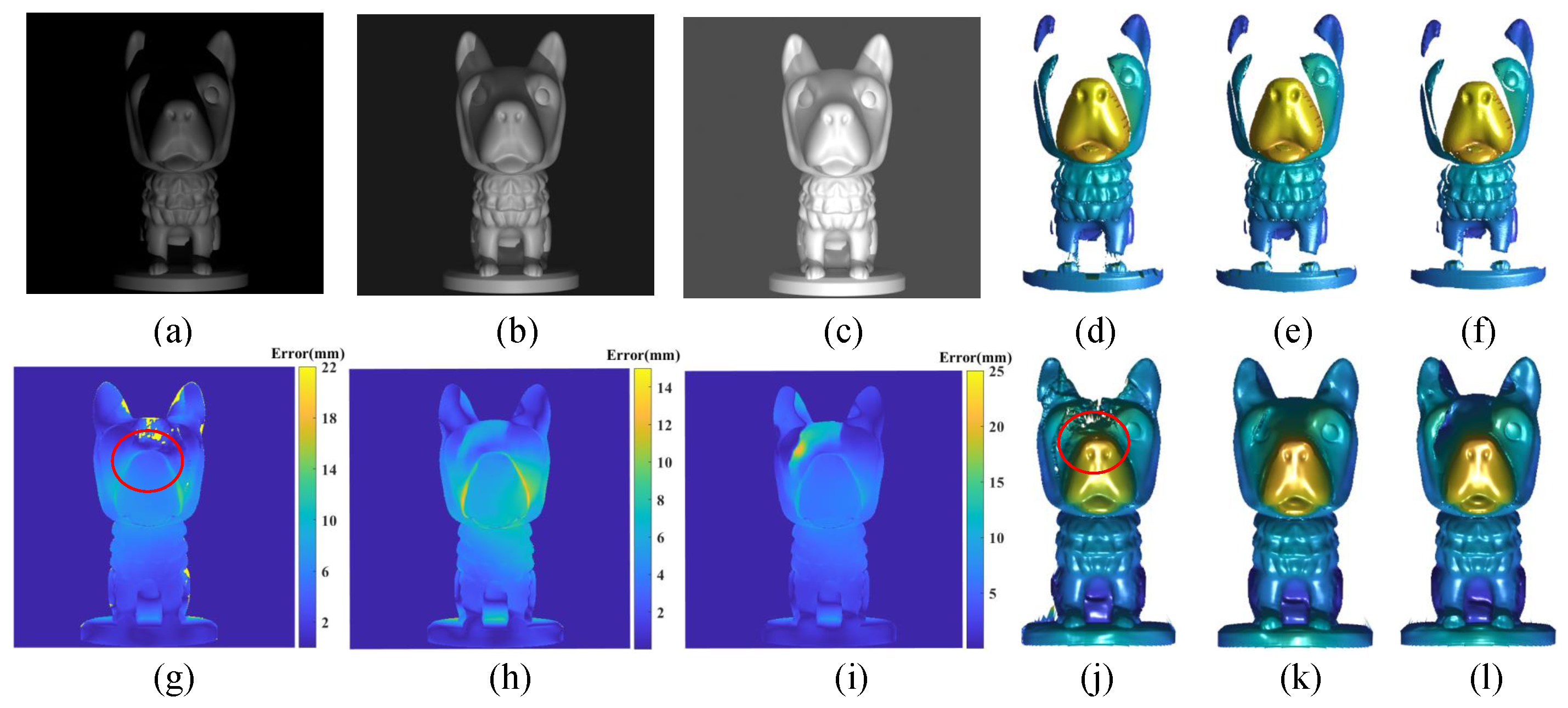
5.1. Influence of Environment Light on Prediction

When we tested the model with data from the real-world FPP system, we found the filled surface was not smooth, and we assumed the low ambient light makes the shadow area of the texture image completely dark so that the contribution from the texture-dominant branch is limited. To test this idea, we deployed the same pre-trained model to the data captured at the same virtual FPP system with different ambient light intensities. We set the ambient light intensity of the virtual FPP system at three different levels: without ambient light, the same ambient light strength utilized to generate the training data, and the strong ambient light that nearly saturates the texture image. The texture images at the three different ambient light intensities are shown in Figure 7a–c. As shown in Figure 7a, the shadow area is dark, and little valid information exists, as almost all lights are blocked. From Figure 7a to Figure 7c, the shadow area becomes lighter, and global image intensity increases with the increase of environment light. However, despite this variation, the phase maps remain identical, and the 3D reconstructed geometries by using the FPP method are presented in Figure 7d–f. Masks are generated based on the depth threshold, which is not influenced by the light intensity, so the mask and the phase map are unchanged among the input data, and the ambient light strength change impacts only the texture image. The 3D reconstructed geometries from the predicted phase maps are illustrated in Figure 7j–l. Compared to the 3D geometry in Figure 7d, our model remedies the holes in the foot area but leaves the holes in the face area of the object, and the filled surface is not smooth. When the ambient light increases and the texture image can provide more information about the shadow area to our model, the holes in the face area are filled, and the filled surface is smoother. The RMSEs of the predicted depth maps for the three cases are $12.5076$ mm, $4.7793$ mm, and $5.2146$ mm, respectively, which also supports that appropriately increasing ambient light strength can improve the model’s performance. The RMSE of the predicted depth map in strong ambient light is higher than in normal ambient light, indicating that high ambient light intensity also limits the model’s performance.

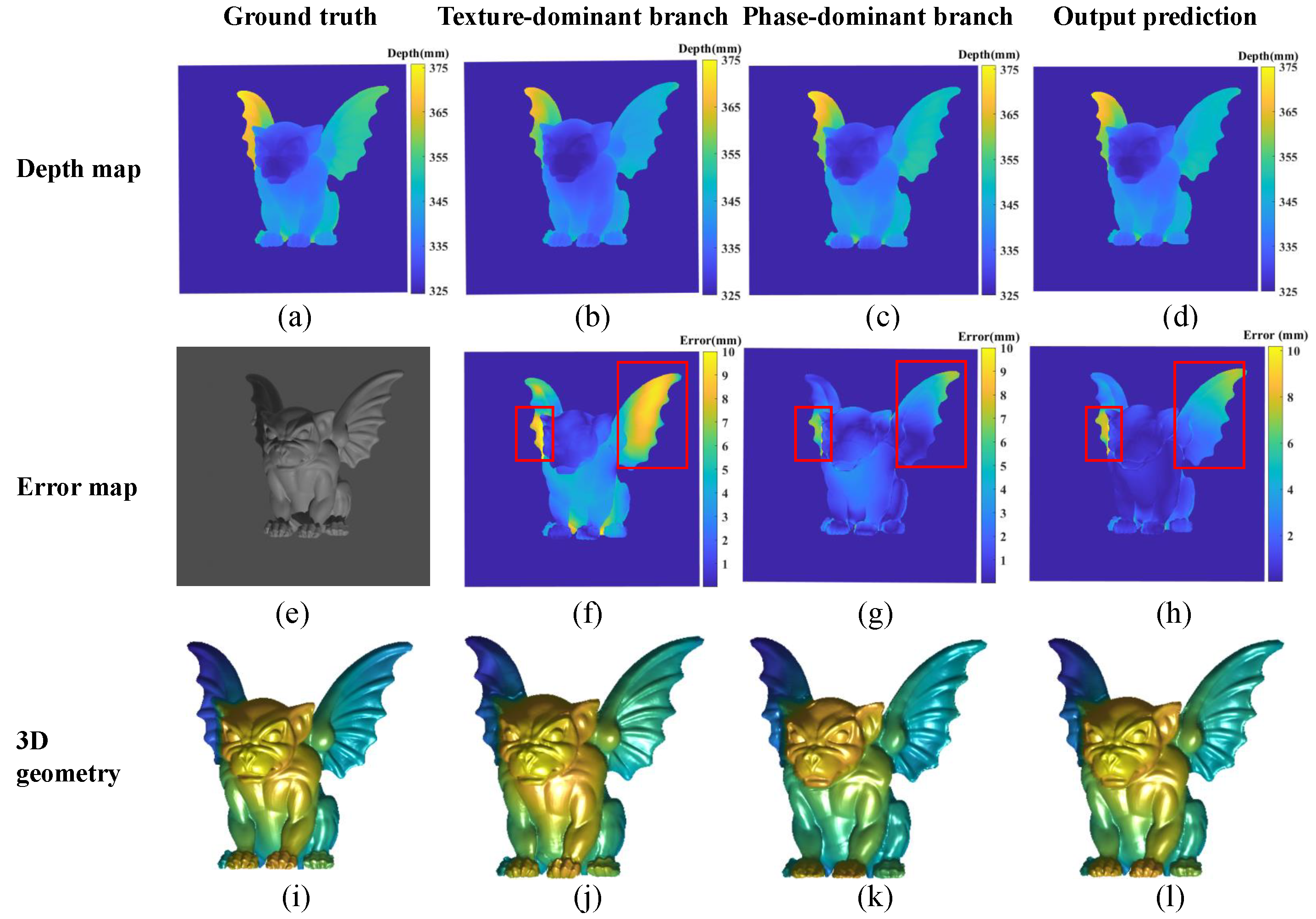
5.2. Function Comparison of the Two Branch Networks

As presented in experiments, our model can convert phase maps to depth maps and reduce shadow-induced errors by combining the texture-dominant branch network and the phase-dominant branch network. We are curious about how each branch network contributes to the output predictions. Thus, we compared the results from each branch as illustrated in Figure 8. Figure 8f,g depict the absolute error of the results from the texture-dominant branch and phase-dominant branch, respectively. The texture-dominant branch network can produce detailed predictions for the whole object, even for the shadow-covered area. The RMSE of the texture-dominant branch is $4.7078$ mm, with most of the discrepancies concentrated on the gargoyle’s wings. Compared to the texture-dominant branch network, the RMSE of the depth map from the phase-dominant branch network is much lower at $2.4269$ mm, and the absolute error on the wings of the object in Figure 8g is more lower than in Figure 8f. Thus, the phase-dominant branch network can make more accurate predictions. Based on the investigation in Section 5.1, the texture-dominant branch network can extract features in shadow-covered areas to remedy the shadow-induced errors in predictions. As we use two weight maps to combine the two depth maps and generate the final output prediction, the RMSE of the final output is $RMSE$: 2.6485 mm, which is higher than the result from the phase-dominant branch network and much lower than the result from the texture-dominant branch network. Therefore, the texture-dominant branch network can extract features from the texture images to repair shadow-induced errors, but makes a lower-quality prediction of the object. The phase-dominant branch can produce relatively accurate predictions, and it needs features from the texture-dominant branch network to make predictions for the shadow-covered area.

6. Conclusions

Shadow-induced errors in phase maps can lead to inaccurate 3D reconstruction in measurements taken using fringe projection profilometry (FPP), thereby invalidating the results. Various approaches have been proposed to address this issue, including incorporating extra devices or making the camera and projector uniaxial to prevent shadow generation, removing shadow-induced errors directly from phase maps and leaving gaps in 3D reconstruction, and smoothing errors using interpolation or similar techniques. However, in this study, we propose a deep learning model that can convert phase maps to depth maps and rectify shadow-induced errors. We validate the efficacy of our model using both virtual scanning data and real-world experiments. Our contributions are as follows:

• Texture images are leveraged as guidance for shadow-induced error removal, and information from phase maps and texture images are combined at two stages.
• A specified loss function that combines image edge details and structural similarity is designed to better train the model.

However, our proposed model has certain limitations. For instance, the model’s performance is influenced by the intensity of ambient light, and may not be able to extract valid information from texture images under low or high ambient light conditions. Moreover, the accuracy of our model is lower than that of FPP in non-shadow regions, indicating that it does not directly use information from the phase branch. On the other hand, our model has the advantage of making predictions for the entire object rather than just the shadow-covered regions, without requiring any additional preprocessing such as shadow detection or image semantic segmentation.

Future research directions could focus on developing end-to-end deep learning models that can obtain depth maps from captured images and rectify shadow-induced errors, as well as combining FPP and deep learning methods to rectify shadow-induced errors without compromising accuracy in non-shadow regions. To improve the generalization ability of the model, researchers can utilize data from diverse virtual systems [44] or consider the camera-projector system’s parameters when designing the network. Our proposed model provides a useful reference for researchers working on related tasks in the FPP system.

References

1. Zuo, C.; Feng, S.; Huang, L.; Tao, T.; Yin, W.; Chen, Q. Phase shifting algorithms for fringe projection profilometry: A review. Opt. Lasers Eng. 2018, 109, 23–59. [Google Scholar] [CrossRef]
2. Xu, J.; Zhang, S. Status, challenges, and future perspectives of fringe projection profilometry. Opt. Lasers Eng. 2020, 135, 106193. [Google Scholar] [CrossRef]
3. Jing, H.; Su, X.; You, Z. Uniaxial three-dimensional shape measurement with multioperation modes for different modulation algorithms. Opt. Eng. 2017, 56, 034115. [Google Scholar] [CrossRef]
4. Zheng, Y.; Li, B. Uniaxial High-Speed Microscale Three-Dimensional Surface Topographical Measurements Using Fringe Projection. J. Micro Nano-Manuf. 2020, 8, 041007. [Google Scholar] [CrossRef]
5. Meng, W.; Quanyao, H.; Yongkai, Y.; Yang, Y.; Qijian, T.; Xiang, P.; Xiaoli, L. Large DOF microscopic fringe projection profilometry with a coaxial light-field structure. Opt. Express 2022, 30, 8015–8026. [Google Scholar] [CrossRef] [PubMed]
6. Skydan, O.A.; Lalor, M.J.; Burton, D.R. Using coloured structured light in 3-D surface measurement. Opt. Lasers Eng. 2005, 43, 801–814. [Google Scholar] [CrossRef]
7. Weinmann, M.; Schwartz, C.; Ruiters, R.; Klein, R. A multi-camera, multi-projector super-resolution framework for structured light. In Proceedings of the 2011 International Conference on 3D Imaging, Modeling, Processing, Visualization and Transmission, Hangzhou, China, 16–19 May 2011; pp. 397–404. [Google Scholar]
8. Huang, L.; Asundi, A.K. Phase invalidity identification framework with the temporal phase unwrapping method. Meas. Sci. Technol. 2011, 22, 035304. [Google Scholar] [CrossRef]
9. Lu, L.; Xi, J.; Yu, Y.; Guo, Q.; Yin, Y.; Song, L. Shadow removal method for phase-shifting profilometry. Appl. Opt. 2015, 54, 6059–6064. [Google Scholar] [CrossRef] [Green Version]
10. Shi, B.; Ma, Z.; Liu, J.; Ni, X.; Xiao, W.; Liu, H. Shadow Extraction Method Based on Multi-Information Fusion and Discrete Wavelet Transform. IEEE Trans. Instrum. Meas. 2022, 71, 1–15. [Google Scholar] [CrossRef]
11. Zhang, S. Phase unwrapping error reduction framework for a multiple-wavelength phase-shifting algorithm. Opt. Eng. 2009, 48, 105601. [Google Scholar] [CrossRef]
12. Chen, F.; Su, X.; Xiang, L. Analysis and identification of phase error in phase measuring profilometry. Opt. Express 2010, 18, 11300–11307. [Google Scholar] [CrossRef] [PubMed]
13. Sun, Z.; Jin, Y.; Duan, M.; Kan, Y.; Zhu, C.; Chen, E. Discriminative repair approach to remove shadow-induced error for typical digital fringe projection. Opt. Express 2020, 28, 26076–26090. [Google Scholar] [CrossRef] [PubMed]
14. Zuo, C.; Qian, J.; Feng, S.; Yin, W.; Li, Y.; Fan, P.; Han, J.; Qian, K.; Chen, Q. Deep learning in optical metrology: A review. Light. Sci. Appl. 2022, 11, 1–54. [Google Scholar]
15. Yan, K.; Yu, Y.; Huang, C.; Sui, L.; Qian, K.; Asundi, A. Fringe pattern denoising based on deep learning. Opt. Commun. 2019, 437, 148–152. [Google Scholar] [CrossRef]
16. Yang, T.; Zhang, Z.; Li, H.; Li, X.; Zhou, X. Single-shot phase extraction for fringe projection profilometry using deep convolutional generative adversarial network. Meas. Sci. Technol. 2020, 32, 015007. [Google Scholar] [CrossRef]
17. Li, Y.; Qian, J.; Feng, S.; Chen, Q.; Zuo, C. Single-shot spatial frequency multiplex fringe pattern for phase unwrapping using deep learning. In Proceedings of the Optics Frontier Online 2020: Optics Imaging and Display, Shanghai, China, 19–20 June 2020; Volume 11571, pp. 314–319. [Google Scholar]
18. Zhang, Q.; Lu, S.; Li, J.; Li, W.; Li, D.; Lu, X.; Zhong, L.; Tian, J. Deep phase shifter for quantitative phase imaging. arXiv 2020, arXiv:2003.03027. [Google Scholar]
19. Wang, K.; Li, Y.; Kemao, Q.; Di, J.; Zhao, J. One-step robust deep learning phase unwrapping. Opt. Express 2019, 27, 15100–15115. [Google Scholar] [CrossRef] [PubMed]
20. Spoorthi, G.; Gorthi, S.; Gorthi, R.K.S.S. PhaseNet: A deep convolutional neural network for two-dimensional phase unwrapping. IEEE Signal Process. Lett. 2018, 26, 54–58. [Google Scholar] [CrossRef]
21. Yan, K.; Yu, Y.; Sun, T.; Asundi, A.; Kemao, Q. Wrapped phase denoising using convolutional neural networks. Opt. Lasers Eng. 2020, 128, 105999. [Google Scholar] [CrossRef]
22. Montresor, S.; Tahon, M.; Laurent, A.; Picart, P. Computational de-noising based on deep learning for phase data in digital holographic interferometry. APL Photonics 2020, 5, 030802. [Google Scholar] [CrossRef] [Green Version]
23. Li, Z.w.; Shi, Y.s.; Wang, C.j.; Qin, D.h.; Huang, K. Complex object 3D measurement based on phase-shifting and a neural network. Opt. Commun. 2009, 282, 2699–2706. [Google Scholar] [CrossRef]
24. Van der Jeught, S.; Dirckx, J.J. Deep neural networks for single shot structured light profilometry. Opt. Express 2019, 27, 17091–17101. [Google Scholar] [CrossRef] [PubMed]
25. Nguyen, H.; Wang, Y.; Wang, Z. Single-shot 3D shape reconstruction using structured light and deep convolutional neural networks. Sensors 2020, 20, 3718. [Google Scholar] [CrossRef] [PubMed]
26. Zheng, Y.; Wang, S.; Li, Q.; Li, B. Fringe projection profilometry by conducting deep learning from its digital twin. Opt. Express 2020, 28, 36568–36583. [Google Scholar] [CrossRef]
27. Elharrouss, O.; Almaadeed, N.; Al-Maadeed, S.; Akbari, Y. Image inpainting: A review. Neural Process. Lett. 2020, 51, 2007–2028. [Google Scholar] [CrossRef] [Green Version]
28. Team, B.D. Blender—A 3D Modelling and Rendering Package; Blender Foundation, Stichting Blender Foundation: Amsterdam, The Netherlands, 2018. [Google Scholar]
29. Wang, C.; Pang, Q. The elimination of errors caused by shadow in fringe projection profilometry based on deep learning. Opt. Lasers Eng. 2022, 159, 107203. [Google Scholar] [CrossRef]
30. Malacara, D. Optical Shop Testing; John Wiley & Sons: Hoboken, NJ, USA, 2007; Volume 59. [Google Scholar]
31. Wang, Y.; Zhang, S.; Oliver, J.H. 3D shape measurement technique for multiple rapidly moving objects. Opt. Express 2011, 19, 8539–8545. [Google Scholar] [CrossRef] [Green Version]
32. Zheng, Y.; Zhang, X.; Wang, S.; Li, Q.; Qin, H.; Li, B. Similarity evaluation of topography measurement results by different optical metrology technologies for additive manufactured parts. Opt. Lasers Eng. 2020, 126, 105920. [Google Scholar] [CrossRef] [Green Version]
33. Hu, M.; Wang, S.; Li, B.; Ning, S.; Fan, L.; Gong, X. Penet: Towards precise and efficient image guided depth completion. In Proceedings of the 2021 IEEE International Conference on Robotics and Automation (ICRA), Xi’an, China, 30 May–5 June 2021; pp. 13656–13662. [Google Scholar]
34. Ronneberger, O.; Fischer, P.; Brox, T. U-net: Convolutional networks for biomedical image segmentation. In Proceedings of the International Conference on Medical Image Computing and Computer-Assisted Intervention, Munich, Germany, 5–9 October 2015; pp. 234–241. [Google Scholar]
35. He, K.; Zhang, X.; Ren, S.; Sun, J. Deep residual learning for image recognition. In Proceedings of the IEEE Conference on Computer Vision and Pattern Recognition, Las Vegas, NV, USA, 27–30 June 2016; pp. 770–778. [Google Scholar]
36. Van Gansbeke, W.; Neven, D.; De Brabandere, B.; Van Gool, L. Sparse and noisy lidar completion with rgb guidance and uncertainty. In Proceedings of the 2019 16th International Conference on Machine Vision Applications (MVA), Tokyo, Japan, 27–31 May 2019; pp. 1–6. [Google Scholar]
37. Zhao, H.; Gallo, O.; Frosio, I.; Kautz, J. Loss functions for image restoration with neural networks. IEEE Trans. Comput. Imaging 2016, 3, 47–57. [Google Scholar] [CrossRef]
38. Wang, Z.; Bovik, A.C.; Sheikh, H.R.; Simoncelli, E.P. Image quality assessment: From error visibility to structural similarity. IEEE Trans. Image Process. 2004, 13, 600–612. [Google Scholar] [CrossRef] [Green Version]
39. Bojanowski, P.; Joulin, A.; Lopez-Paz, D.; Szlam, A. Optimizing the latent space of generative networks. arXiv 2017, arXiv:1707.05776. [Google Scholar]
40. Zhou, Q.; Jacobson, A. Thingi10K: A Dataset of 10,000 3D-Printing Models. arXiv 2016, arXiv:1605.04797. [Google Scholar]
41. Free 3D Models. Available online: https://free3d.com/3d-models/ (accessed on 10 May 2022).
42. Paszke, A.; Gross, S.; Massa, F.; Lerer, A.; Bradbury, J.; Chanan, G.; Killeen, T.; Lin, Z.; Gimelshein, N.; Antiga, L.; et al. Pytorch: An imperative style, high-performance deep learning library. In Advances in Neural Information Processing Systems; Neural Information Processing Systems Foundation, Inc. (NeurIPS): Vancouver, BC, Canada, 2019; Volume 32. [Google Scholar]
43. Robbins, H.; Monro, S. A stochastic approximation method. Ann. Math. Stat. 1951, 22, 400–407. [Google Scholar] [CrossRef]
44. Wang, F.; Wang, C.; Guan, Q. Single-shot fringe projection profilometry based on deep learning and computer graphics. Opt. Express 2021, 29, 8024–8040. [Google Scholar] [CrossRef] [PubMed]
Figure 1. Illustration of the formation of shadows and shadow-induced errors in FPP. (a) The formation of shadows; (b) Shadow-induced errors in the wrapped phase map; (c) 3D reconstructed geometry with holes.
Photonics 10 00246 g001
Figure 2. Schematic of the proposed model.
Photonics 10 00246 g002
Figure 3. One sample in the dataset. (ac) Three phase-shifting fringe patterns projected on an object; (di) Six gray code images projected on an object; (j) The corresponding texture image; (k,l) The corresponding wrapped phase map and unwrapped phase map; (m) The mask generated by a depth threshold; (n) The corresponding ground truth (the depth map directly exported from the virtual system).
Photonics 10 00246 g003
Figure 4. Results of an object from the virtual scanning. (ac) The input of the texture image, the mask, and the phase map; (df) 3D geometry from FPP, the ground truth, and the prediction; (g) The ground truth of the depth map; (h) The predicted depth map; (i) The absolute error map with RMSE 2.6485 mm.
Photonics 10 00246 g004
Figure 5. Effectiveness evaluation of the proposed model for scanning a single object in the real-world FPP system. (a) Texture image; (b) Unwrapped phase map; (c) 3D reconstructed geometry from FPP; (d) The depth map from FPP; (e) The error map for the non-shadow covered region with RMSE 1.5031 mm; (f) 3D reconstructed geometry from the predicted depth map.
Photonics 10 00246 g005
Figure 6. Effectiveness evaluation of the proposed model for scanning two objects in the real-world FPP system. (a) Texture image; (b) Unwrapped phase map; (c) 3D reconstructed geometry from FPP; (d) The depth map from FPP; (e) The error map for the non-shadow covered region with RMSE 2.3579 mm; (f) 3D reconstructed geometry from the predicted depth map.
Photonics 10 00246 g006
Figure 7. Predictions under different intensity levels of ambient light. (a) The texture image obtained without ambient light; (b) The texture image obtained with the same ambient light intensity as the training data; (c) The texture image obtained with strong ambient light to make it close to saturation; (df) 3D reconstructed geometries by using the FPP method for the three cases; (gi) Absolute error maps for the three cases by comparing ground truths and the predicted depth maps, with RMSE 12.5076 mm, 4.7793 mm and 5.2146 mm, respectively; (jl) 3D reconstructed geometries from the predicted depth maps for the three cases.
Photonics 10 00246 g007
Figure 8. Comparing functions of the texture-dominant branch and phase-dominant branch. (ad) Depth maps of the ground truth, texture-dominant branch, phase-dominant branch, and the output prediction; (e) Texture image; (fh) Absolute error maps of (bd) with RMSE 4.7078 mm, 2.4269 mm and 2.6485 mm, respectively; (il) 3D geometries from the ground truth, the texture-dominant branch’s prediction, the phase-dominant branch’s prediction, and the output prediction.
Photonics 10 00246 g008