Communication

CoolMomentum-SPGD Algorithm for Wavefront Sensor-Less Adaptive Optics Systems

1
School of Electronic Engineering, Jiangsu Ocean University, Lianyungang 222005, China
2
School of Network & Telecom Engineering, Jinling Institute of Technology, Nanjing 211169, China
*
Author to whom correspondence should be addressed.
Photonics 2023, 10(2), 102; https://doi.org/10.3390/photonics10020102
Submission received: 30 November 2022 / Revised: 12 January 2023 / Accepted: 12 January 2023 / Published: 18 January 2023

Abstract

:
Instead of acquiring the previous aberrations of an optical wavefront with a sensor, wavefront sensor-less (WFSless) adaptive optics (AO) systems compensate for wavefront distortion by optimizing the performance metric directly. The stochastic parallel gradient descent (SPGD) algorithm is pervasively adopted to achieve performance metric optimization. In this work, we incorporate CoolMomentum, a method for stochastic optimization by Langevin dynamics with simulated annealing, into SPGD. Numerical simulations reveal that, compared with the state-of-the-art SPGD variant, the proposed CoolMomentum-SPGD algorithm achieves better convergence speed under various atmospheric turbulence conditions while requiring only two tunable parameters.

1. Introduction

Adaptive optics (AO) [1] technology reduces optical wavefront distortions with deformable mirrors (DMs) or spatial light modulators (SLMs). It is used in astronomical telescopes and free-space optical communication (FSO) to mitigate the effect brought about by atmospheric turbulence [2,3]. Fluorescence microscopy adopts AO technology to reduce optical aberrations introduced by the refractive index structure of specimens [4]. Retinal imaging adopts AO technology to compensate for the eye’s optical aberrations, enabling an unprecedented visualization of retinal structures [5]. Laser processing uses AO technology to correct for aberrations introduced when focusing lasers onto workpieces, bringing about tailored focal intensity distribution [6]. Extreme ultraviolet lithography uses AO technology to mitigate aberrations induced by the thermal deformation of a mirror [7]. In the field of structured light, AO technology shows promise in both phase and polarization error correction, providing a solution for the highly flexible generation of structured light fields [8,9].
Basically, there are two paradigms in applying AO technology. As for the conventional paradigm [10], a wavefront sensor, whose role is to sense the aberration of an optical wavefront, is indispensable. The aberration is then compensated by applying a conjugate phase. The other paradigm exerts wavefront control instruction according to direct system performance metric optimization [11]. A wavefront sensor is absent in this paradigm; hence, wavefront sensor-less (WFSless) AO is realized [12]. WFSless AO enjoys substantial benefits in circumstances where a wavefront sensor is inapplicable, or where strong scintillation is present.
Various gradient-descent methods can be applied to optimize the system performance metric in a WFSless AO system. Among them, the stochastic parallel gradient descent (SPGD) [13,14] optimization algorithm is pervasively recognized as a promising method. As for SPGD, the control elements introduce stochastic parallel perturbations into the optical system, and a set of performance metrics is measured with a photodetector. The extremum of the performance metric is achieved by the adaptation of the correction elements after numerous iterations. In such a manner, the effect of wavefront distortions is eliminated. For each iteration in the optimization process, control voltages exerted on the correction elements are determined by the gradient estimation of the system performance metric, a predefined or adaptive gain of step size, and the history of control voltages. Aside from effective convergence, the efficiency of the SPGD algorithm is a significant concern. Constant endeavors have been made to accelerate the iteration process.
Along with the advent of SPGD, two approaches for algorithm acceleration have already been proposed by Vorontsov [15]. One approach brings in an additional low-resolution modal wavefront corrector, which excels at dealing with large-scale aberrations efficiently. The other approach utilizes global coupling, i.e., each correction element participates in both local and global wavefront control. The possibility of an adaptive gain, or learning rate in the field of machine learning, has also been explored extensively. Carhart has constructed an adaptive gain according to the change in system performance metric [16], which indicates whether the optimization process is in a transition state or a stationary state. Different gains are preferred in those states, respectively. A hybrid gain composed of the sign, absolute value, and previous increment of the system performance metric change has been proposed by Weyrauch et al. [17]. With the development of deep learning, various optimizers have been proposed to train neural networks. Many of the proposed optimizers, e.g., Momentum [18,19], Adagrad [20,21], Adam [22,23], and Nadam [24], have been successfully incorporated into the SPGD algorithm, bringing about an acceleration of the iteration process. The effectiveness of these SPGD variants has been verified theoretically and experimentally. Among the adopted optimizers, Adam and its sibling Nadam achieve the best performance [25,26,27].
CoolMomentum [28] is a method for stochastic optimization by Langevin dynamics with simulated annealing, recently proposed by Borysenko from the Kharkiv Institute of Physics and Technology, Ukraine. In this paper, we adapt CoolMomentum to conventional SPGD, thus proposing a new SPGD variant algorithm coined CoolMomentum-SPGD, which achieves better performance on both iteration efficiency and convergence accuracy than the state-of-the-art algorithms under various atmospheric turbulence conditions. Meanwhile, the proposed CoolMomentum-SPGD algorithm requires only two tunable parameters, which indicates it is technically more feasible than the four-parameter Adam and Nadam SPGD variants.

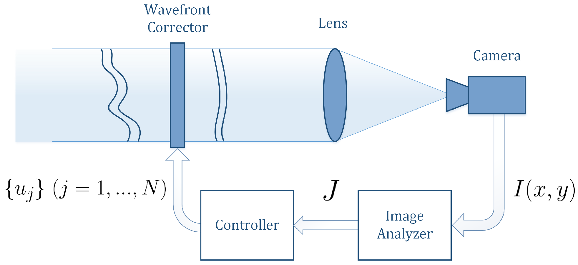
2. Materials and Methods

In the absence of a stand-alone wavefront sensor, WFSless AO develops the control schemes of the wavefront corrector according to far-field images acquired with a camera. Each image is then formulated as a scalar performance metric. Thus, the problem of eliminating wavefront distortion is treated as maximizing/minimizing the specific performance metric. By deliberately introducing prescribed voltage perturbations to the wavefront corrector, the consequent variance in the performance metrics may be utilized to determine the proper voltages to be exerted on the actuating elements of the wavefront corrector. In this way, WFSless AO eliminates wavefront aberrations by direct system performance metric optimization. A typical WFSless AO system configuration is illustrated in Figure 1.
For a wavefront corrector with N elements, a far-field image I ( x , y ) is acquired after control voltages { u j } ( j = 1 , , N ) are applied. The image I ( x , y ) is then analyzed to form a performance metric J. Therefore, J is a function of the control voltages { u j } ( j = 1 , , N ) :
J = J ( u 1 , , u j , , u N ) j = 1 , , N .
To optimize J, various gradient descent approaches are available. As for the conventional SPGD [15] algorithm, stochastic small perturbations { δ u j } ( j = 1 , , N ) are exerted in parallel to the control voltages { u j } ( j = 1 , , N ) . All perturbations share the same magnitude: | δ u j | = δ u , while the signs of perturbations are randomly chosen with equal probability for δ u j = δ u and δ u j = δ u . In actual practice, bilateral perturbations are often applied. To begin with, perturbations { δ u j } ( j = 1 , , N ) are applied to get a corresponding performance metric J + . Then, perturbations in the other direction are applied to get an oppositely perturbed performance metric J . To explicitly indicate the iterative steps, a superscript n is added. Therefore, we have
J + ( n ) = J ( u 1 ( n ) + δ u 1 ( n ) , , u j ( n ) + δ u j ( n ) , , u N ( n ) + δ u N ( n ) )
and
J ( n ) = J ( u 1 ( n ) δ u 1 ( n ) , , u j ( n ) δ u j ( n ) , , u N ( n ) δ u N ( n ) ) .
Performance metric variation δ J = J + J is adopted to help estimate the gradient. Specifically, δ J δ u j is a proven reasonable approximation of the gradient [15]. In this way, the iterative procedure of the conventional SPGD algorithm can be expressed as
u j ( n + 1 ) = u j ( n ) + γ δ J ( n ) δ u j ( n ) , j = 1 , , N .
in which γ is a gain coefficient (i.e., learning rate) that scales the degree of updates. γ is positive for performance metric maximization and negative otherwise. The second component γ δ J ( n ) δ u j ( n ) is the required update of the voltage on every control element. When expressed in vector form, this component may be replaced with a single vector Δ u ( n + 1 ) for simplicity.
SPGD is pervasively recognized as an effective method for performance metric optimization. Meanwhile, endeavors have always been made to accelerate the iteration process. The momentum of inertia and adaptive learning rates are the most common considerations, such as those exploited in Momentum-SPGD [20] and Adam-SPGD [22]. Recently, Borysenko proposed a method for stochastic optimization by Langevin dynamics with simulated annealing, namely CoolMomentum [28]. According to Langevin dynamics,
4 T ( 1 ρ ) / ( 1 + ρ ) = c o n s t ,
in which T is the temperature, and ρ is the coefficient of momentum. By gradually decreasing the momentum coefficient ρ in the optimization procedure, ( 1 ρ ) / ( 1 + ρ ) increases accordingly. According to Equation (5), T decreases. Therefore, simulated annealing, or cooling, is achieved implicitly. That is where the name “CoolMomentum” comes from. Different cooling strategies are available, among which a promising one is
ρ ( n ) = 1 ( 1 ρ 0 ) / α n .
The initial momentum coefficient ρ 0 is predefined manually. The decreasing rate of the momentum coefficient ρ ( n ) depends on the hyperparameter α , or “cooling rate”. On the condition that ρ ( n ) decreases to zero at the last iteration step, for an altogether S-step iteration procedure the cooling rate α is set as
α = ( 1 ρ 0 ) 1 / S .
With this delicately chosen α , the momentum component vanishes when the iteration procedure ends, and the implicit temperature decreases to its minimum as well. When transforming the Langevin equation into the form of the Momentum optimization algorithm, the learning rate comes to its advent. The relation between learning rate l r ( n ) and momentum coefficient ρ n is inherently constrained by Langevin dynamics, which expresses as
l r ( n ) = l r 0 · 1 + ρ ( n ) 2 ,
in which l r 0 is a manually predefined initial learning rate. For every iteration step, the momentum coefficient ρ ( n ) is determined by Equation (6); hence, cooling down occurs. Then, the learning rate l r ( n ) updates itself according to the value of ρ ( n ) , as in Equation (8).
Incorporating the momentum coefficient ρ ( n ) and learning rate l r ( n ) into the conventional SPGD algorithm (Equation (4)), we propose the CoolMomentum-SPGD algorithm. Algorithm 1 illustrates the thorough procedure.
Algorithm 1 CoolMomentum-SPGD
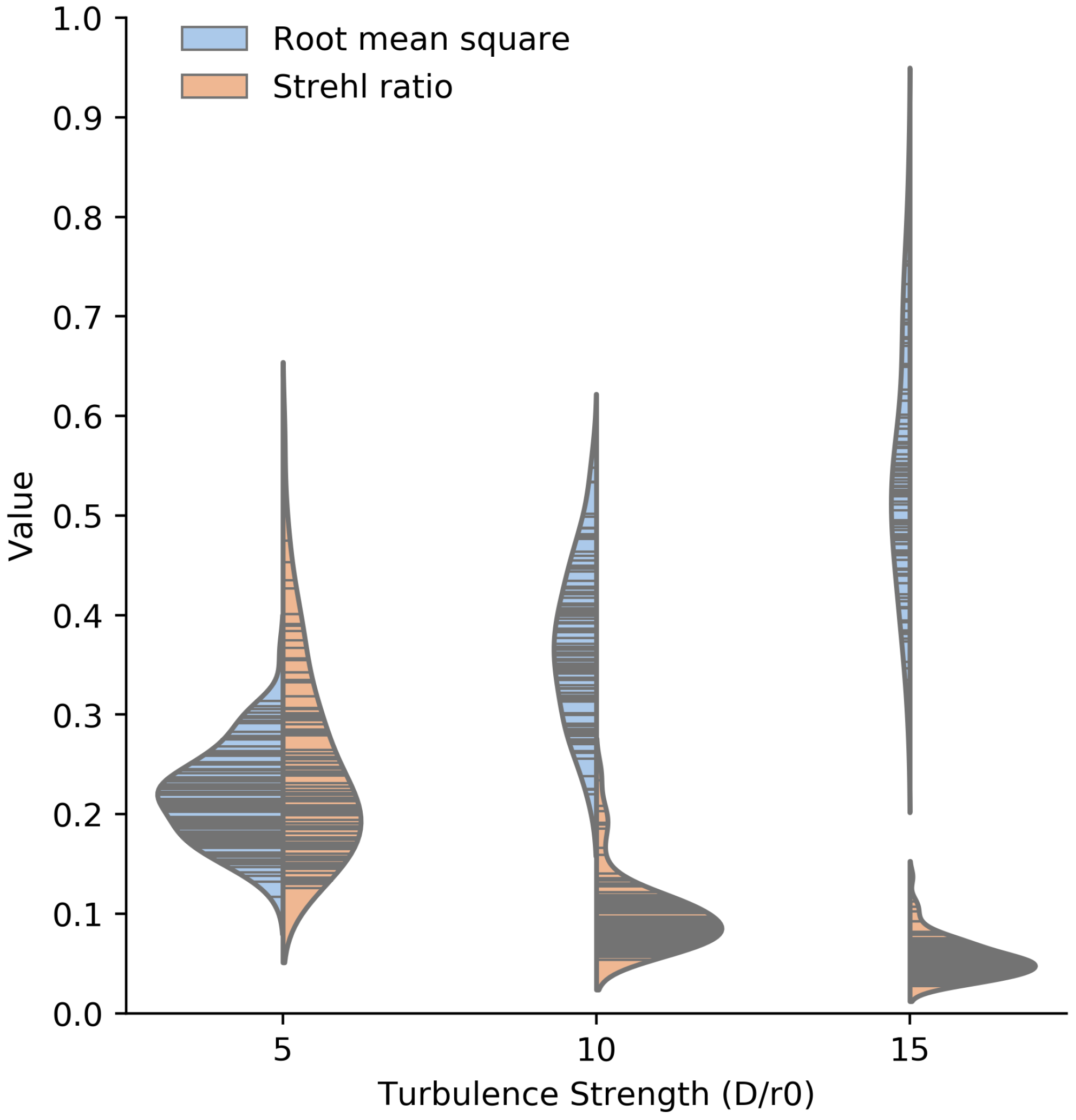
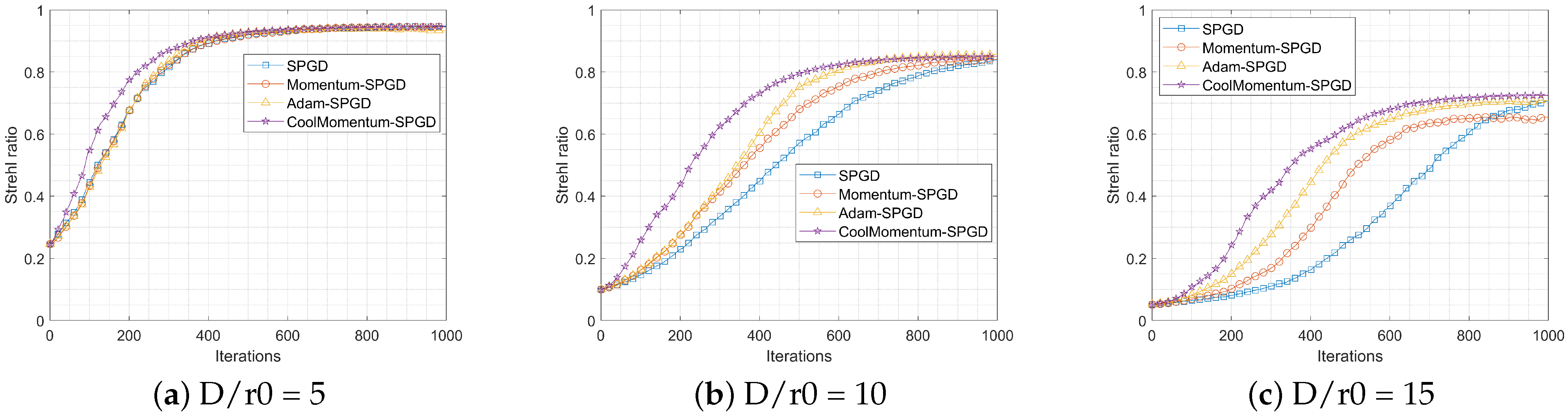
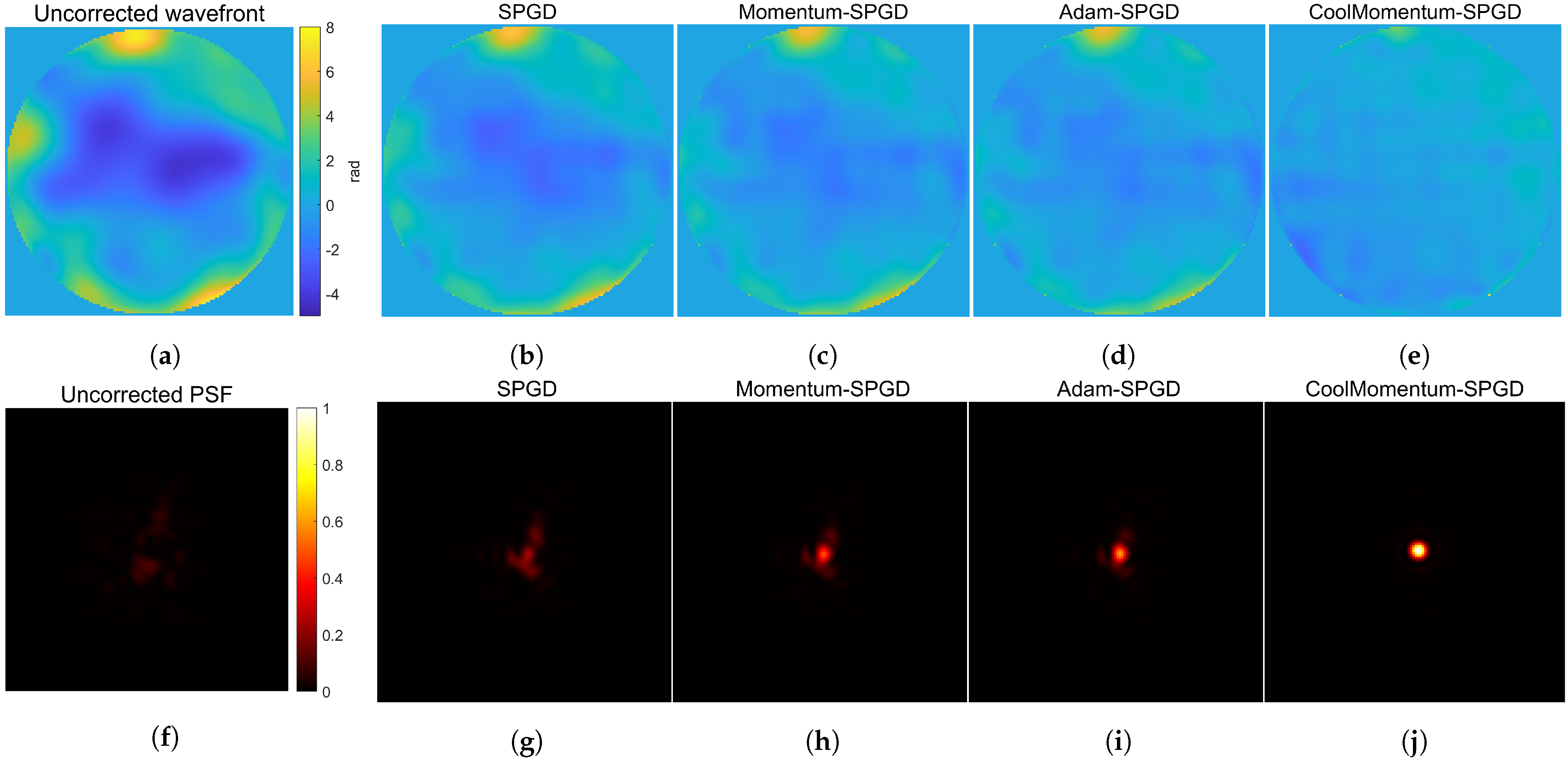
Require: 
l r 0 (initial learning rate),   ρ 0 (initial momentum coefficient)
  • Set { u j } = 0 ( j = 1 , , N ) ,
  • Set  { Δ u j } = 0 ( j = 1 , , N ) , in which N is the number of corrector channels
  • Compute α = ( 1 ρ 0 ) 1 / S , in which S is the number of iterations to perform
  • for  n = 1 , , S   do
  •      ρ ( n ) = max 0 , 1 ( 1 ρ 0 ) / α n
  •      l r ( n ) = l r 0 · ( 1 + ρ ( n ) ) / 2
  •      J + ( n ) = J ( u 1 ( n ) + δ u 1 ( n ) , , u j ( n ) + δ u j ( n ) , , u N ( n ) + δ u N ( n ) )
  •      J ( n ) = J ( u 1 ( n ) δ u 1 ( n ) , , u j ( n ) δ u j ( n ) , , u N ( n ) δ u N ( n ) )
  •      δ J ( n ) = J + ( n ) J ( n )
  •      Δ u j ( n + 1 ) = ρ ( n ) Δ u j ( n ) + l r ( n ) δ J ( n ) δ u j ( n )
  •      u j ( n + 1 ) = u j ( n ) + Δ u j ( n + 1 )
  • end for
It is worth noting that only two tunable parameters are required, i.e., the initial learning rate l r 0 and initial momentum coefficient ρ 0 . Identifying the most favorable set of tunable parameters is quite laborious. Therefore, having fewer parameters will be a great benefit for practical application. The predefined tunable parameters of four typical algorithms are compared in Table 1. The conventional SPGD algorithm merely has a sole parameter—the learning rate l r . Momentum-SPGD and CoolMomentum-SPGD have two parameters, respectively—learning rate and momentum coefficient. In contrast, the renowned Adam-SPGD has four tunable parameters. In the next section, the performances of the SPGD algorithm and its variant algorithms are thoroughly compared.

3. Results

To confirm the superiority of our CoolMomentum-SPGD algorithm, adequate numerical simulations have been performed. A sum of 100 Kolmogorov phase screens under turbulence strength D / r 0 = 5, 10, and 15 are generated, respectively [30]. D is the aperture diameter of the receiver, and r 0 is the atmospheric coherent length. Statistics of the simulated phase screens are depicted with a violin plot (Figure 2). Two metrics, i.e., the root mean square (RMS) error and initial Strehl ratio of the AO system with simulated phase screens, are provided in pairs under different atmospheric turbulence strengths. The unit of measurement is common for the two metrics. Every stick in the violin plot indicates an instance of the simulated phase screens. The difference in turbulence strengths manifests well in statistical distribution.
To perform SPGD or any of its variant algorithms, a performance metric J (Figure 1) must be specified. Here, the mean radius of the intensity distribution [31] measured by the camera is adopted. Thus, the performance metric is expressed as
J = ( x x 0 ) 2 + ( y y 0 ) 2 I ( x , y ) d x d y I ( x , y ) d x d y ,
in which I ( x , y ) is the two-dimensional intensity distribution, and ( x 0 , y 0 ) is the centroid of I ( x , y ) . This performance metric is measured repetitively in the iterative procedures of all evaluated algorithms hereafter.
To evaluate the performance of the proposed CoolMomentum-SPGD algorithm, we compare it with three other representative counterparts—conventional SPGD, Momentum-SPGD, and Adam-SPGD. The reason for choosing the Momentum-SPGD algorithm as a basis of comparison lies in the fact that Momentum-SPGD is not only a typical improvement on conventional SPGD (by introducing momentum components into the iterative procedure) but also a degraded version of CoolMomentum-SPGD (without cooling the momentum components). At the same time, Adam-SPGD is chosen as a benchmark since it is pervasively acknowledged as state-of-the-art [25,27]. Numerical simulations are performed under three different atmospheric turbulence strengths. The parameters of each algorithm (as in Table 1) are determined through a brute-force search for each circumstance. The range and interval of the brute-force search are determined empirically. Accordingly, for each turbulence strength, every algorithm has been tuned for its optimal performance.
The characteristics of a 97-element deformable mirror are introduced to perform the simulations. Figure 3 illustrates the obtained averaged Strehl ratio adaptation curves. Except for Momentum-SPGD under turbulence strength D/r0 = 15, all other curves converge to global extrema. It is worth noting that, under each atmospheric circumstance, CoolMomentum-SPGD achieves the fastest convergence without exception. Under weak turbulence circumstances (Figure 3a), the other three algorithms perform almost the same, while CoolMomentum-SPGD still maintains a recognizable lead. When turbulence is moderate (Figure 3b), the superiority of CoolMomentum-SPGD over other curves is especially obvious. Even with severe turbulence (Figure 3c), CoolMomentum-SPGD still holds the lead through the whole iterative process.
To evaluate the performance of CoolMomentum-SPGD more intuitively, a typical phase screen generated under turbulence strength D/r0 = 10 is picked out. The initial uncorrected wavefront and its corresponding far-field Point Spread Function (PSF) are provided in Figure 4a,f, respectively. The aforementioned four algorithms are applied separately. The number of iterations is set to 400 deliberately, which is far from adequate for each algorithm to converge. It is obvious that after 400 iterations CoolMomentum-SPGD eliminates the wavefront aberration effectively and the corresponding far-field PSF takes shape well. CoolMomentum-SPGD outperforms other algorithms notably. Actually, the outcome of the performance evaluation based on the wavefront and PSF (Figure 4) is in accordance with the Strehl ratio curves in Figure 3b.
To investigate every single realization of the wavefront correction process, the Strehl ratio adaptation curves of 100 realizations for each iterative optimization algorithm are provided, respectively (Figure 5). The atmospheric turbulence strength is D/r = 10 for all of these realizations. It is shown that, even for a specific atmospheric turbulence strength, the realization curves of SPGD and those of Momentum-SPGD diverge considerably (Figure 5a,b). In other words, although the averaged curve indicates a reasonable performance, for some realizations (lower blue curves) conventional SPGD and Momentum-SPGD lose their effectiveness. In contrast, the realization curves of Adam-SPGD and CoolMomentum-SPGD are much more concentrated. Figure 5c,d demonstrate the effectiveness of Adam-SPGD and CoolMomentum-SPGD in most cases. The performance difference between Adam-SPGD and CoolMomentum-SPGD is not quite significant. Basically, with CoolMomentum-SPGD the realization curves tend to rise more abruptly at the beginning of the iterative procedure, leading to a faster convergence speed than Adam-SPGD. The root of CoolMomentum-SPGD’s performance advantage over Adam-SPGD will be discussed in Section 4.
The capability of eliminating wavefront aberration, i.e., convergence effectivity at the end of the iterative procedure, is illustrated in Figure 6. The Strehl ratio curves of the initial uncorrected wavefront (green) and the ideally corrected wavefront with a 97-element deformable mirror (black) are also provided for reference. Under various atmospheric turbulence circumstances, all of the evaluated algorithms are able to eliminate the wavefront aberration effectively, leading to a substantial increase in the Strehl ratio over the initial curve. Except for Momentum-SPGD’s slight underperformance when D/r0 is 15, there is no apparent difference between the evaluated algorithms under every specific turbulence circumstance. At the end of the iterative procedure, CoolMomentum-SPGD does not outperform its rivals, whereas its performance advantage is basically on convergence speed, as demonstrated in Figure 3 and Figure 5. It is worth noting that CoolMomentum-SPGD surpasses the renowned Adam-SPGD in convergence speed with only two tunable parameters.

4. Discussion

To investigate the root of CoolMomentum-SPGD’s impressive performance, it is beneficial to inspect the step size in the iterative procedures. The Euclidean norm is adopted to measure the length of each step, i.e., the update of the control voltage vector Δ u ( n + 1 ) . Figure 7 illustrates every step size Δ u ( n + 1 ) during the whole iterative procedure of each evaluated algorithm. Several thought-provoking comparisons can be made:
  • SPGD vs. others. The adjacent step size varies abruptly in the iterative procedure of SPGD (Figure 7a), whereas it shows much more consistency between adjacent steps for the other three algorithms. The consistency of step size is essentially due to taking the momentum of inertia into account, as in the case of Momentum-SPGD, Adam-SPGD, and CoolMomentum-SPGD.
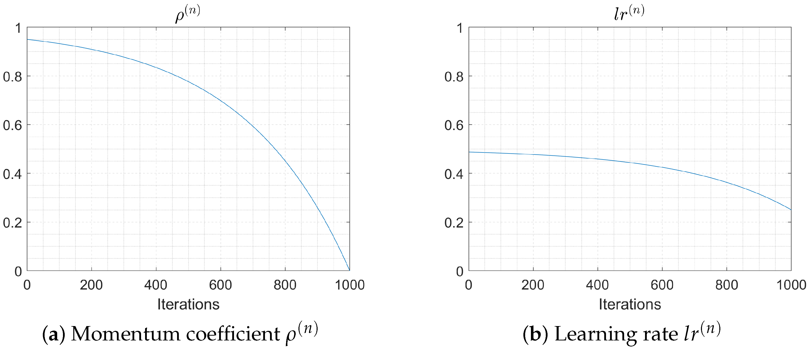
  • CoolMomentum-SPGD vs. Momentum-SPGD. For Momentum-SPGD, the step size is generally even in the whole iterative procedure (Figure 7b). For CoolMomentum-SPGD, the step size behaves in a bold manner in the early stage, while it descends gradually into a negligible magnitude in the later stage (Figure 7d). This dramatic decline in step size originates from the “cooling” operation of the inertial momentum. It is worth comparing the crucial iterative schemes of Momentum-SPGD and CoolMomentum-SPGD.
    Momentum-SPGD:
    Δ u j ( n + 1 ) = ρ Δ u j ( n ) + l r δ J ( n ) δ u j ( n ) ,
    u j ( n + 1 ) = u j ( n ) + Δ u j ( n + 1 ) .
    CoolMomentum-SPGD:
    Δ u j ( n + 1 ) = ρ ( n ) Δ u j ( n ) + l r ( n ) δ J ( n ) δ u j ( n ) ,
    u j ( n + 1 ) = u j ( n ) + Δ u j ( n + 1 ) .
    The expressions of Momentum-SPGD and CoolMomentum-SPGD are quite similar. The update of control voltage Δ u j ( n + 1 ) consists of two parts, the inertial momentum of the past updates and the gradient scaled by a learning rate. Thus, either of the algorithms has two parameters, a momentum coefficient and a learning rate. However, the momentum coefficient and learning rate for Momentum-SPGD are both fixed, while those for CoolMomentum-SPGD are variable through the iterative procedure. Figure 8 illustrates ρ ( n ) and the corresponding l r ( n ) (according to Equation (8)) in a typical iterative procedure of CoolMomentum-SPGD. The “cooling” of the momentum is prominent in Figure 8a. It is this cooling momentum that leads to the decaying step size in Figure 7d, as well as the superiority in convergence speed. It is worth noting that ρ ( n ) and l r ( n ) are determined by their initial values ρ 0 and l r 0 , respectively. Therefore, two predefined parameters are needed to implement CoolMomentum-SPGD, which is the same as Momentum-SPGD.
  • CoolMomentum-SPGD vs. Adam-SPGD. Both of the algorithms take into account the inertial momentum and possess adaptive learning rates, by which remarkable performance is achieved. Adam-SPGD’s adaptive learning rate originates from the division by cumulative squared gradients [32]. In contrast, CoolMomentum-SPGD’s adaptive learning rate stems from the cooling momentum (Equation (8)). According to the above numerical simulations, CoolMomentum-SPGD’s scheme achieves better convergence speed than Adam-SPGD’s in controlling wavefront correctors, despite the fact that fewer tunable parameters are required.

5. Conclusions

Increasing the convergence speed of the iterative optimization algorithms adopted in controlling the wavefront correctors in WFSless AO systems is of great significance. In this paper, we propose a new SPGD variant algorithm, which is coined CoolMomentum-SPGD. Numerical simulations have been made to compare our algorithm with several representative counterparts. It is demonstrated that CoolMomentum-SPGD converges faster than others under various atmospheric turbulence conditions (Figure 3). With inadequate iterations, it eliminates wavefront aberration effectively (Figure 4). It is worth noting that CoolMomentum-SPGD outperforms the renowned Adam-SPGD algorithm. In addition, CoolMomentum-SPGD requires fewer tunable parameters than Adam-SPGD, which makes it practically more promising. Furthermore, the step size during the whole iterative procedure of each evaluated algorithm has been inspected. The discussion on step size sheds light upon the distinct performances of the algorithms.

Author Contributions

Conceptualization, Z.Z. and H.Y.; methodology, Z.Z.; software, Y.L.; validation, H.S., J.L.; resources, H.Y.; writing—original draft preparation, Z.Z.; writing—review and editing, H.Y.; funding acquisition, H.Y. All authors have read and agreed to the published version of the manuscript.

Funding

This research was funded by the National Natural Science Foundation of China (grant number U2141255).

Institutional Review Board Statement

Not applicable.

Informed Consent Statement

Not applicable.

Data Availability Statement

The data presented in this study are available on request from the corresponding author.

Acknowledgments

We attribute our work to Borysenko, who proposed CoolMomentum. Borysenko is from the Kharkiv Institute of Physics and Technology, Ukraine. We wish him safe and sheltered.

Conflicts of Interest

The authors declare no conflict of interest.

References

  1. Tyson, R.K.; Frazier, B.W. Principles of Adaptive Optics; CRC Press: Boca Raton, FL, USA, 2022. [Google Scholar]
  2. Madec, P.Y. Overview of deformable mirror technologies for adaptive optics and astronomy. In Adaptive Optics Systems III; SPIE: Bellingham, WA, USA, 2012; Volume 8447, pp. 22–39. [Google Scholar]
  3. Martínez, N.; Ramos, L.F.R.; Sodnik, Z. Simulating the performance of adaptive optics techniques on FSO communications through the atmosphere. In Laser Communication and Propagation through the Atmosphere and Oceans VI; SPIE: Bellingham, WA, USA, 2017; Volume 10408, pp. 49–57. [Google Scholar]
  4. Booth, M.J.; Débarre, D.; Jesacher, A. Adaptive Optics for Biomedical Microscopy. Opt. Photon. News 2012, 23, 22–29. [Google Scholar] [CrossRef]
  5. Godara, P.; Dubis, A.M.; Roorda, A.; Duncan, J.L.; Carroll, J. Adaptive optics retinal imaging: Emerging clinical applications. Optom. Vis. Sci. Off. Publ. Am. Acad. Optom. 2010, 87, 930. [Google Scholar] [CrossRef] [PubMed] [Green Version]
  6. Salter, P.S.; Booth, M.J. Adaptive optics in laser processing. Light Sci. Appl. 2019, 8, 110. [Google Scholar] [PubMed] [Green Version]
  7. Habets, M.; Scholten, J.; Weiland, S.; Coene, W. Multi-mirror adaptive optics for control of thermally induced aberrations in extreme ultraviolet lithography. In Extreme Ultraviolet (EUV) Lithography VII; SPIE: Bellingham, WA, USA, 2016; Volume 9776, pp. 662–673. [Google Scholar]
  8. He, C.; Shen, Y.; Forbes, A. Towards higher-dimensional structured light. Light Sci. Appl. 2022, 11, 205. [Google Scholar] [CrossRef]
  9. Grunwald, R.; Jurke, M.; Bock, M.; Liebmann, M.; Bruno, B.P.; Gowda, H.; Wallrabe, U. High-Flexibility Control of Structured Light with Combined Adaptive Optical Systems. Photonics 2022, 9, 42. [Google Scholar] [CrossRef]
  10. Primot, J. Theoretical description of Shack–Hartmann wave-front sensor. Opt. Commun. 2003, 222, 81–92. [Google Scholar] [CrossRef]
  11. Antonello, J.; van Werkhoven, T.; Verhaegen, M.; Truong, H.H.; Keller, C.U.; Gerritsen, H.C. Optimization-based wavefront sensorless adaptive optics for multiphoton microscopy. J. Opt. Soc. Am. A 2014, 31, 1337–1347. [Google Scholar] [CrossRef] [Green Version]
  12. Yang, H.; Soloviev, O.; Verhaegen, M. Model-based wavefront sensorless adaptive optics system for large aberrations and extended objects. Opt. Express 2015, 23, 24587–24601. [Google Scholar] [CrossRef]
  13. Vorontsov, M.A.; Carhart, G.W.; Ricklin, J.C. Adaptive phase-distortion correction based on parallel gradient-descent optimization. Opt. Lett. 1997, 22, 907. [Google Scholar] [CrossRef]
  14. Yang, H.; Li, X.; Gong, C.; Jiang, W. Restoration of turbulence-degraded extended object using the stochastic parallel gradient descent algorithm: Numerical simulation. Opt. Express 2009, 17, 3052–3062. [Google Scholar] [CrossRef]
  15. Vorontsov, M.A.; Sivokon, V.P. Stochastic parallel-gradient-descent technique for high-resolution wave-front phase-distortion correction. J. Opt. Soc. Am. A 1998, 15, 2745–2758. [Google Scholar] [CrossRef]
  16. Carhart, G.W.; Vorontsov, M.A.; Cohen, M.H.; Cauwenberghs, G.; Edwards, R.T. Adaptive wavefront correction using a VLSI implementation of the parallel gradient descent algorithm. In High-Resolution Wavefront Control: Methods, Devices, and Applications; Gonglewski, J.D., Vorontsov, M.A., Eds.; International Society for Optics and Photonics, SPIE: Bellingham, WA, USA, 1999; Volume 3760, pp. 61–66. [Google Scholar] [CrossRef]
  17. Weyrauch, T.; Vorontsov, M.A.; Bifano, T.G.; Giles, M.K. Adaptive optics system with micromachined mirror array and stochastic gradient descent controller. In High-Resolution Wavefront Control: Methods, Devices, and Applications II; Gonglewski, J.D., Vorontsov, M.A., Gruneisen, M.T., Eds.; International Society for Optics and Photonics, SPIE: Bellingham, WA, USA, 2000; Volume 4124, pp. 178–188. [Google Scholar] [CrossRef]
  18. Yang, G.; Liu, L.; Jiang, Z.; Guo, J.; Wang, T. Incoherent beam combining based on the momentum SPGD algorithm. Opt. Laser Technol. 2018, 101, 372–378. [Google Scholar] [CrossRef]
  19. Song, J.; Li, Y.; Che, D.; Guo, J.; Wang, T. Coherent beam combining based on the SPGD algorithm with a momentum term. Optik 2020, 202, 163650. [Google Scholar] [CrossRef]
  20. Song, J.; Li, Y.; Che, D.; Wang, T. Numerical and experimental study on coherent beam combining using an improved stochastic parallel gradient descent algorithm. Laser Phys. 2020, 30, 085102. [Google Scholar] [CrossRef]
  21. Che, D.; Li, Y.; Wu, Y.; Song, J.; Wang, T. Theory of AdmSPGD algorithm in fiber laser coherent synthesis. Opt. Commun. 2021, 492, 126953. [Google Scholar] [CrossRef]
  22. Fang, Z.; Xu, X.; Li, X.; Yang, H.; Gong, C. SPGD algorithm optimization based on Adam optimizer. In AOPC 2020: Optical Sensing and Imaging Technology; Luo, X., Jiang, Y., Lu, J., Liu, D., Eds.; International Society for Optics and Photonics, SPIE: Bellingham, WA, USA, 2020; Volume 11567, p. 115672S. [Google Scholar] [CrossRef]
  23. Hu, Q.; Zhen, L.; Mao, Y.; Zhu, S.; Zhou, X.; Zhou, G. Adaptive stochastic parallel gradient descent approach for efficient fiber coupling. Opt. Express 2020, 28, 13141–13154. [Google Scholar] [CrossRef] [PubMed]
  24. Xu, L.; Wang, J.; Yang, L.; Zhang, H. Design and Performance Analysis of NadamSPGD Algorithm for Sensor-Less Adaptive Optics in Coherent FSOC Systems. Photonics 2022, 9, 77. [Google Scholar] [CrossRef]
  25. Zhao, H.; An, J.; Yu, M.; Lv, D.; Kuang, K.; Zhang, T. Nesterov-accelerated adaptive momentum estimation-based wavefront distortion correction algorithm. Appl. Opt. 2021, 60, 7177–7185. [Google Scholar] [CrossRef]
  26. Zhang, H.; Xu, L.; Guo, Y.; Cao, J.; Liu, W.; Yang, L. Application of AdamSPGD algorithm to sensor-less adaptive optics in coherent free-space optical communication system. Opt. Express 2022, 30, 7477. [Google Scholar] [CrossRef]
  27. Wu, J.; Hu, C.; Liu, R.; Wu, S.; Cao, J.; Cheng, Z.; Yu, B.; Zhang, L. Adam SPGD algorithm in freeform surface in-process interferometry. Opt. Express 2022, 30, 32528–32539. [Google Scholar] [CrossRef]
  28. Borysenko, O.; Byshkin, M. CoolMomentum: A method for stochastic optimization by Langevin dynamics with simulated annealing. Sci. Rep. 2021, 11, 10705. [Google Scholar] [CrossRef] [PubMed]
  29. Qian, N. On the momentum term in gradient descent learning algorithms. Neural Netw. 1999, 12, 145–151. [Google Scholar] [CrossRef]
  30. Assémat, F.; Wilson, R.W.; Gendron, E. Method for simulating infinitely long and non stationary phase screens with optimized memory storage. Opt. Express 2006, 14, 988–999. [Google Scholar] [CrossRef] [PubMed]
  31. Jiang, P.; Liang, Y.; Xu, J.; Mao, H. A new performance metric on sensorless adaptive optics imaging system. Optik 2016, 127, 222–226. [Google Scholar] [CrossRef]
  32. Kingma, D.P.; Ba, J. Adam: A Method for Stochastic Optimization. arXiv 2014, arXiv:1412.6980. [Google Scholar] [CrossRef]
Figure 1. Schematic of a wavefront sensor-less (WFSless) adaptive optics (AO) system.
Photonics 10 00102 g001
Figure 2. Statistics of the simulated phase screens. The root mean square (RMS) error and the Strehl ratio are depicted in a violin plot. The left side of the pattern for each turbulence strength indicates RMS distribution. The right side of each pattern indicates the Strehl ratio distribution. The two types of distribution share the same unit of measurement. Every stick denotes a simulated phase screen, the RMS or Strehl ratio of which is indicated by the stick’s level.
Photonics 10 00102 g002
Figure 3. The averaged Strehl ratio adaptation curves of CoolMomentum-SPGD and other counterparts under turbulence strength D/r0 = 5, 10, and 15.
Photonics 10 00102 g003
Figure 4. Wavefront aberration correction and the corresponding far-field point spread function (PSF) of a typical phase screen generated under turbulence strength D/r0 = 10. Four different iterative optimization algorithms are adopted, respectively. The number of iterations is set to 400. (a) Uncorrected wavefront. (b) Wavefront corrected with SPGD. (c) Wavefront corrected with Momentum-SPGD. (d) Wavefront corrected with Adam-SPGD. (e) Wavefront corrected with CoolMomentum-SPGD. (fj) The corresponding PSFs of wavefront (ae), respectively.
Photonics 10 00102 g004
Figure 5. The Strehl ratio adaptation curves of 100 realizations (blue) and the average (red) under turbulence strength D/r0 = 10.
Photonics 10 00102 g005
Figure 6. The capability of eliminating wavefront aberration measured in the Strehl ratio. Initial: the initial Strehl ratio of the AO system with uncorrected wavefront. Ideal: the ideal Strehl ratio possibly achieved with a 97-element deformable mirror.
Photonics 10 00102 g006
Figure 7. Step size Δ u ( n + 1 ) for the ( n + 1 ) -th iteration during the whole iterative procedure of algorithms (a) SPGD, (b) Momentum-SPGD, (c) Adam-SPGD and (d) CoolMomentum-SPGD.
Photonics 10 00102 g007aPhotonics 10 00102 g007b
Figure 8. Critical parameters in the iterative procedure of CoolMomentum-SPGD.
Photonics 10 00102 g008
Table 1. Predefined tunable parameters comparison.
Algorithmparam1param2param3param4
SPGD [15] l r
Momentum-SPGD [29] l r ρ
Adam-SPGD [22] l r β 1 β 2 ϵ
CoolMomentum-SPGD [28] l r 0 ρ 0
Disclaimer/Publisher’s Note: The statements, opinions and data contained in all publications are solely those of the individual author(s) and contributor(s) and not of MDPI and/or the editor(s). MDPI and/or the editor(s) disclaim responsibility for any injury to people or property resulting from any ideas, methods, instructions or products referred to in the content.

