1. Introduction
Multi-Criteria Decision Making (MCDM) as a scientific field is some 60 years old. Its roots are in Goal Programming [
1] and Multi-Attribute Utility Theory (MAUT) [
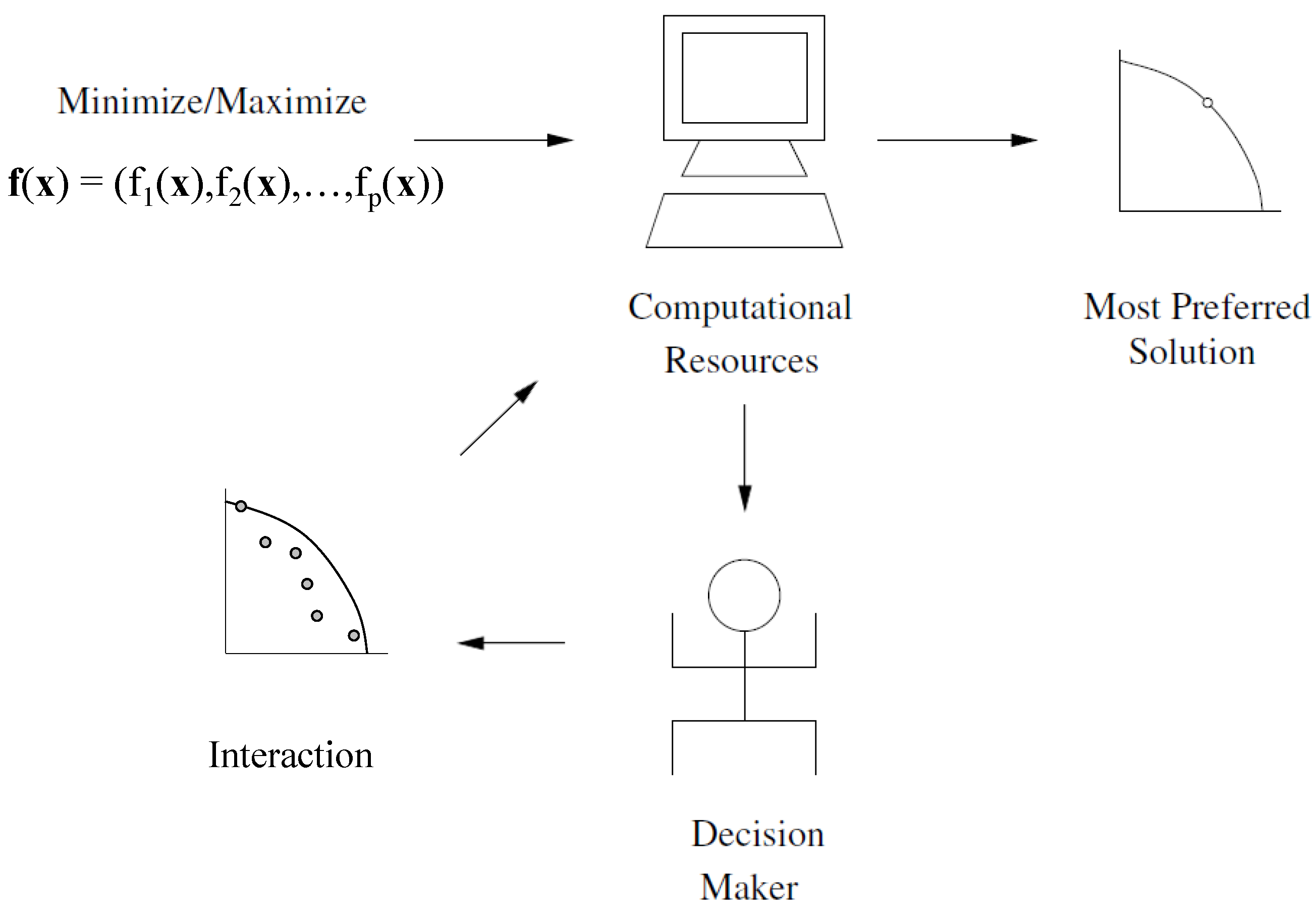
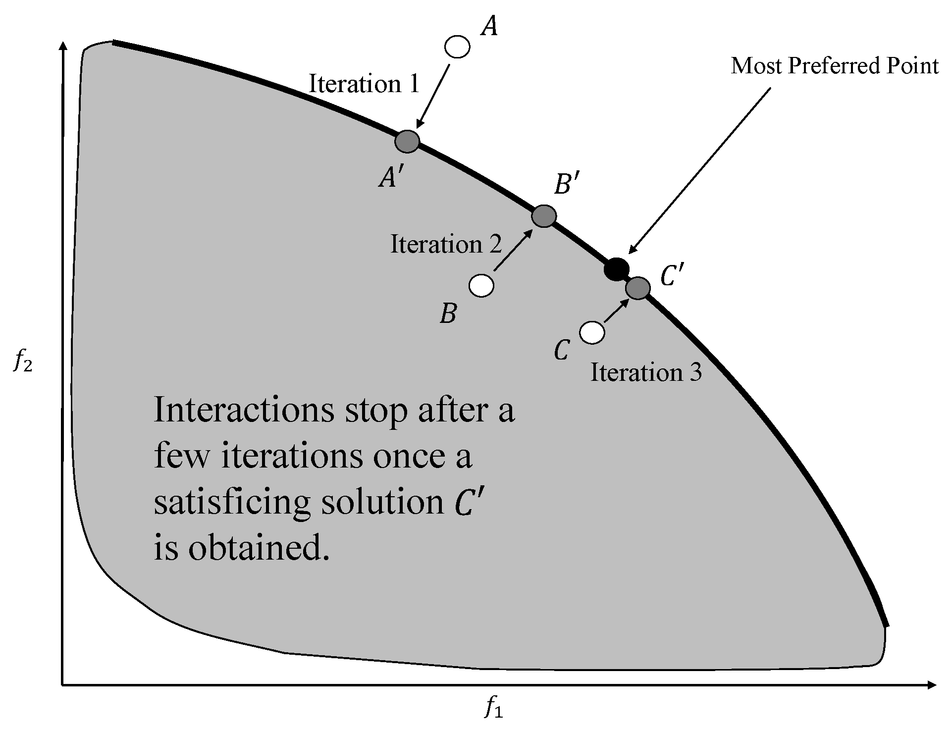
2]. A subsequently popular subfield, interactive man–machine multi-objective optimization, developed greatly during the 1970s. The common frameworks used a discrete set of choices and a mathematical programming problem formulation (optimization) to solve multi-objective problems. With the interactive approaches, phases of decision making and computing would alternate. The aim was to converge towards the most preferred solution on the Pareto-optimal frontier.
Independently from MCDM, the Evolutionary Multi-Objective Optimization (EMO) approaches started developing during the 1980s [
3]. Many of the EMO scholars had an engineering or a computer science background. EMO algorithms [
4,
5] have been applied to problems with multiple objectives for the task of finding a well-representative set of Pareto-optimal solutions. These methods [
6,
7] have been successful in solving a wide variety of problems with two or three objectives. However, these methodologies are criticized for their excessive computational expense, and they often tend to suffer while solving problems with objectives higher than three [
8,
9]. The major hindrances in handling a higher number of objectives relate to stagnation in search, increased dimensionality of Pareto-optimal front, large computational cost, and difficulty in visualization of the objective space. These difficulties are inherent to optimization problems having a large number of objectives and are not easy to eliminate; rather, procedures to handle such difficulties need to be explored. EMO methods that are better equipped at handling a larger number of objectives are being continuously explored [
10,
11,
12]. Some of these approaches aim for solutions that are near Pareto-optimal and provide a discretized and diverse representation of the high-dimensional frontier for many-objective (i.e., more than two or three objectives) problems. However, the level of discretization for an accurate and well-represented many-objective frontier would require a very large number of points. Even if a fine-grained discretization is achieved with a large number of points, the decision-making challenges still remain.
The areas of MCDM and EMO were solving similar problems; therefore, the researchers working in these domains decided to pursue active collaboration through formal channels such as common conferences and seminars. As a result, Branke, Deb, Miettinen, and Słowiński organized the first Dagstuhl seminar [
13] in 2004 to allow collaboration between the two communities. This led to researchers combining ideas from MCDM to EMO and vice-versa. Since then, the Dagstuhl seminar has been organized every few years to enhance the collaboration and flow of ideas from one research community to the other. In this article, we evaluate the classic studies in MCDM and EMO and also the hybrid approaches that have been proposed for handling many-objective problems. Some of the review papers that talk about interactive multi-objective optimization are [
14,
15]. This article takes a tutorial-cum-review approach to discuss the classic ideas published in the areas of MCDM, EMO, and their intersection and is structured as follows. In
Section 2, we cover the theoretical concepts on optimization and decision making that arise in the multi-objective literature. This is followed by
Section 3, where we discuss how search and decision making can be integrated together in various ways to find the most preferred point for the decision maker (DM). Thereafter, we discuss the classic MCDM (
Section 4), EMO (
Section 5), and hybrid (
Section 6) approaches that have been discussed in the literature over the past few decades. We conclude the article in
Section 7 with discussions on behavioral considerations and future work.
2. Multi-Objective Optimization
Multi-objective optimization [
4,
16,
17,
18] involves two or more conflicting objectives that are supposed to be simultaneously optimized subject to a given set of constraints. These problems arise in various fields of science, engineering, economics, and mathematics and have been widely studied in the literature. However, modern applications keep posing challenges with an increasing level of complexity. The complexity depends on a number of factors, such as number of objectives, number of decision variables, type of decision variables (continuous, discrete), number of constraints, and functional form of the functions in the optimization problems (linear, convex, non-convex, non-differentiable, etc.) that may lead to non-separability and multi-modality. While many of the above difficulties are common to single-objective optimization as well, multi-objective optimization poses additional challenges as such problems do not have a single solution which would simultaneously maximize/minimize each of the objectives; instead, there is a set of solutions from which a rational DM should choose. These solutions are called Pareto-optimal solutions. Choosing the most preferred solution from the set of Pareto-optimal solutions requires an additional step of decision making, which is often subjective and not straightforward to model. The challenges posed by multi-objective optimization often include inability to generate a complete ordering of points and requirement of maintaining a pool of non-dominated points. A feasible point in multi-objective optimization is considered to be non-dominated within a set when there does not exist any other feasible point that is better than the former in terms of some objective and is not worse than the former in terms of other objectives. The concept is discussed in detail in
Section 2.1. Difficulty in representation and visualization of the solutions in objective space, especially while working with many objectives, makes decision making difficult, and therefore requires preference learning while searching for the point most preferred by the DM. Below, we describe a general multi-objective problem (
):
In the above formulation, is the n-dimensional decision variable vector which represents the decision space. A search is expected to be performed within the constrained region of the decision space that is determined by the inequality constraints (), equality constraints () and box constraints (). We refer to the set of solutions which are feasible with respect to the constraints and are non-dominated with respect to all feasible solutions, as Pareto-optimal solutions. Among the Pareto-optimal solutions, the solution that is the most preferred by the DM will be referred to as the most preferred solution. We provide formal definitions for these terms in the next sections.
Note that the objective vector is the image of the decision vector under the objective function . In a single-objective optimization () problem, the feasible set is completely ordered according to the objective function , such that for solutions, and in the decision space, either or . Therefore, for two solutions in the objective space, there are two possibilities with respect to the ≥ relation. However, when several objectives () are involved, the feasible set is not necessarily completely ordered but partially ordered. In multi-objective problems, for any two objective vectors, and , the relations => and ≥ can be extended as follows:
⇔ :
⇔ :
⇔ :
While comparing the multi-objective scenario with the single-objective case, we find that for two solutions in the objective space there are three possibilities with respect to the ≥ relation. These possibilities are: , or . If any of the first two possibilities are met, it allows to rank or order the solutions independent of any preference information (or a DM). On the other hand, if the first two possibilities are not met, the solutions cannot be ranked or ordered without incorporating preference information (or involving a DM). Drawing analogy from the above discussion, the relations < and ≤ can be extended in a similar way.
2.1. Dominance Concept
Based on the established binary relations for two vectors in the previous section, the following dominance concept [
16] can be constituted:
strongly dominates ⇔;
(weakly) dominates ⇔;
and are non-dominated with respect to each other ⇔.
In the case of weak dominance, it is common to drop the word
weak and refer to it only with
dominance, which is why we use the word
weak in brackets. Dominance of
over
essentially means that no component of
is less than the corresponding component of
, and at least one component of
is greater than the corresponding component of
. The above dominance concept is also explained in
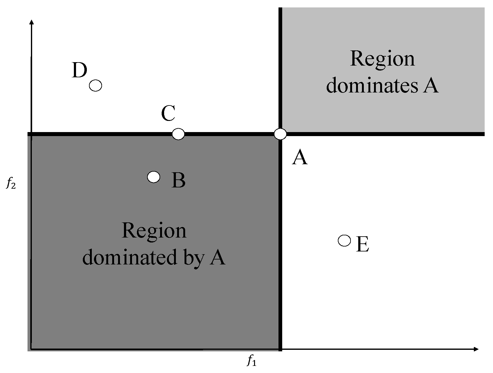
Figure 1 for a two-objective maximization case. In
Figure 1, two shaded regions are shown in reference to point A. The shaded region in the north-east corner (excluding the lines) is the region which strongly dominates point A, the shaded region in the south-west corner (excluding the lines) is strongly dominated by point A, and the non-shaded region is the non-dominated region. Therefore, point A strongly dominates point B, and points A, E, and D are non-dominated with respect to each other. Note that point A weakly dominates point C. From hereon, we only talk about dominance by avoiding the word
weak.
Many of the existing evolutionary multi-objective optimization algorithms use the dominance principle to converge towards the Pareto-optimal set of solutions. The concept allows us to partially order two decision vectors based on the corresponding objective vectors in the absence of any preference information. The algorithms which operate with a sparse set of solutions in the decision space and the corresponding images in the objective space usually give priority to a solution which dominates another solution. The solution which is not dominated with respect to any other solution in the sparse set is referred to as a non-dominated solution within that set.
In case of a discrete set of solutions: the subset whose solutions are not dominated by any solution in the discrete set is referred to as the non-dominated set within the discrete set. When the set in consideration is the entire search space, the resulting non-dominated set is referred to as a Pareto-optimal set, or the frontier formed with these points is referred to as the Pareto-optimal front. To formally define a Pareto-optimal front, consider a set which constitutes the entire decision space with solutions . The subset , containing solutions which are not dominated by any in the entire decision space, forms the Pareto-optimal front.
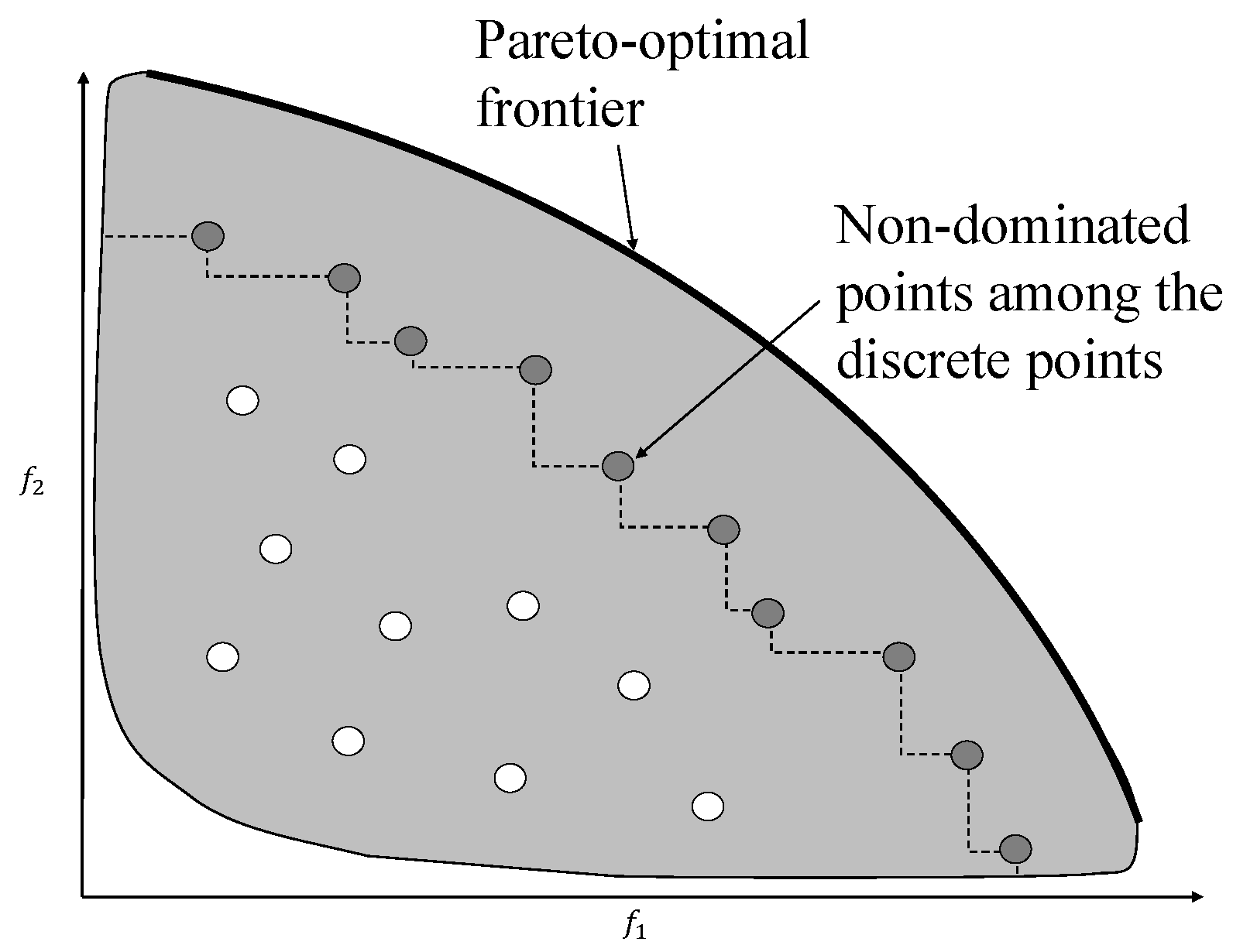
The concept of a Pareto-optimal front and a non-dominated set are illustrated in
Figure 2. The shaded region in the figure represents
. It is the image in the objective space of the entire feasible region in the decision space. The bold curve represents the Pareto-optimal front for a maximization problem. Mathematically, this curve is
, which are all the optimal points for the two objective optimization problem. A number of points are also plotted in the figure, which constitute a discrete set. Among this set of points, the points connected by broken lines are the points which are not dominated by any point in the discrete set. Therefore, these points constitute a non-dominated set within the discrete set. The other points which do not belong to the non-dominated set are dominated by at least one of the points in the non-dominated set.
In the field of MCDM, a Pareto-optimal point in the objective space is often referred to as a non-dominated point, as it is not dominated by any feasible point in the objective space. The corresponding decision vector is referred to as an efficient point. Similarly, if is a dominated point in the objective space, then would be referred to as an inefficient point in the decision space. In other words, a point is efficient if and only if it is the inverse image of a non-dominated objective vector, and it is inefficient if and only if it is an inverse image of a dominated objective vector.
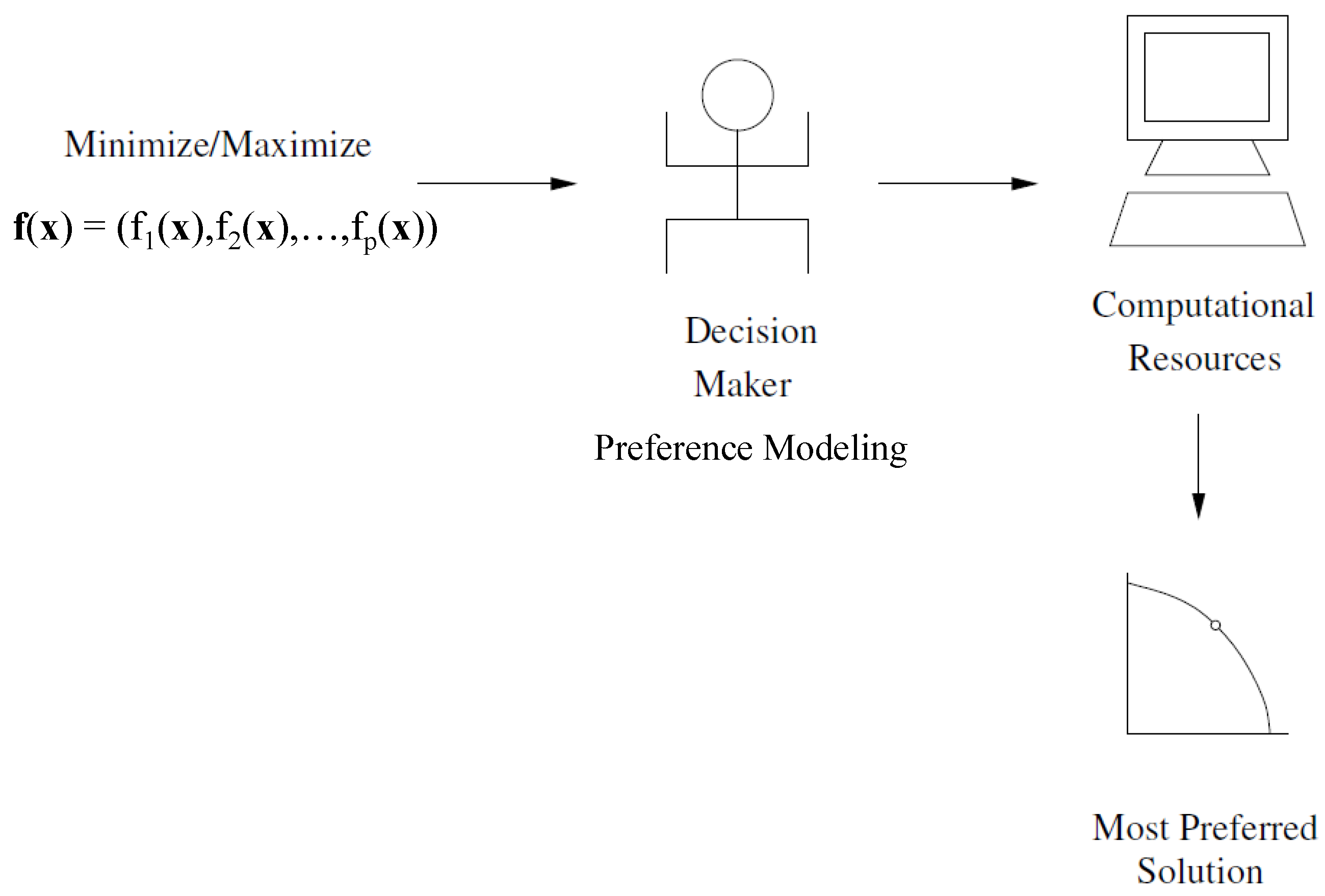
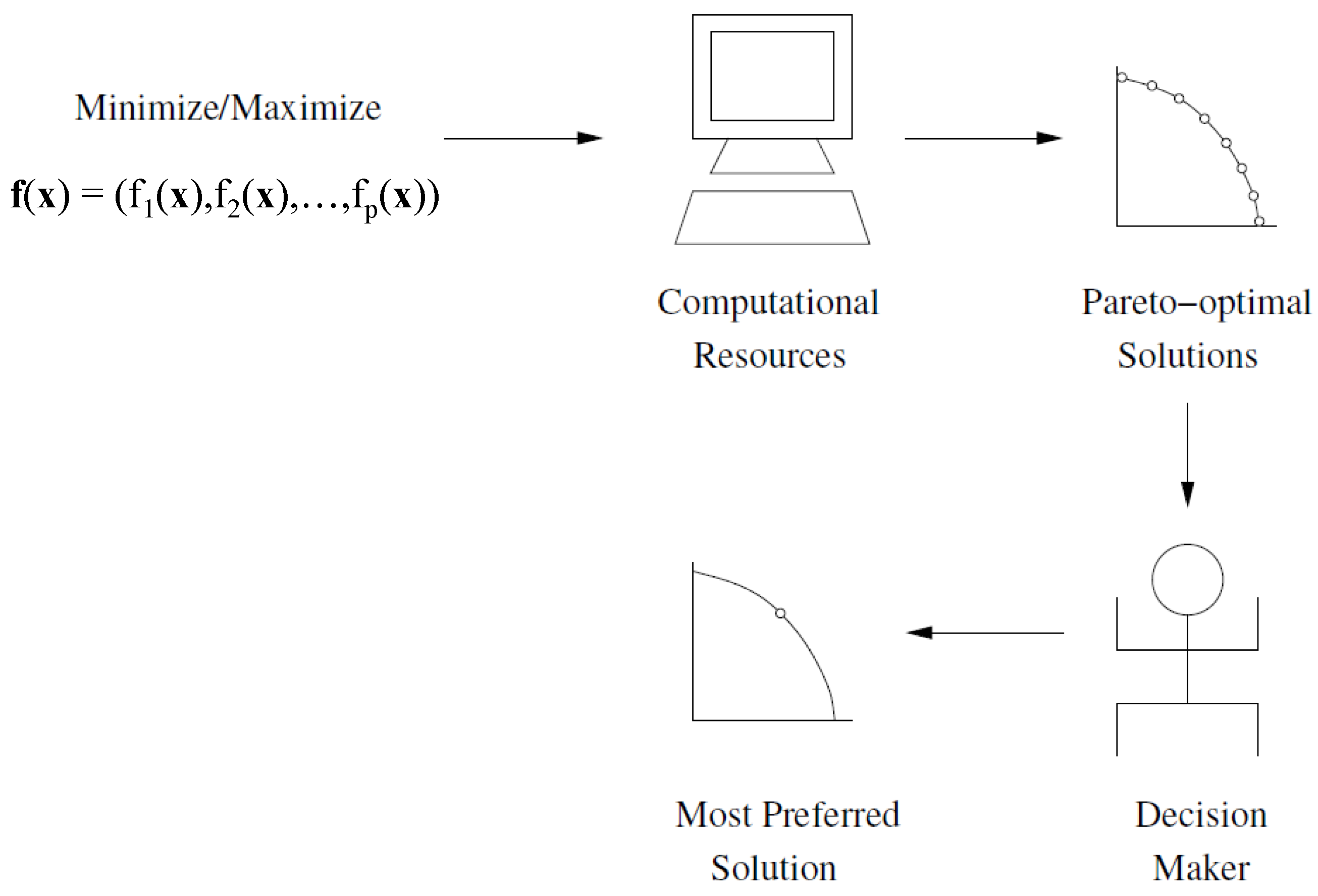
2.2. Decision Making
Even though there are multiple potentially optimal solutions to a multi-objective problem, there is often just a single solution which is of interest to the DM; which is termed as the
most preferred solution. Search and decision making are two intricacies [
19] involved in handling any multi-objective problem. Search requires an intensive exploration in the decision space to get close to the Pareto-optimal solutions; on the other hand, decision making is required to provide preference information over the available non-dominated solutions in pursuance of the most preferred solution.
In a decision-making context, the solutions can be compared and ordered based on the preference information, though there can be situations where strict preference of one solution over the other is not obtained, and the ordering is partial. For instance, consider two vectors, and , in the decision space, having their images, and , in the objective space. A preference structure can be defined using three binary relations ≻, ∼, and ‖. The meaning of the binary relations are provided below:
is preferred over ;
and are equally preferable;
and are incomparable;
where the preference relation, ≻, is asymmetric, the indifference relation, ∼, is reflexive and symmetric, and the incomparability relation, ‖, is irreflexive and symmetric. A weak preference ⪰ relation can be established as such that
As already mentioned, preference can easily be established for pairs where one solution dominates the other. However, for pairs which are non-dominated with respect to each other, a DM’s input is required to establish a preference. The following is the inference for preference choice which can be drawn from dominance:
It is common to emulate a DM with a value function, , which is scalar in nature and assigns a value or a measure of satisfaction to each of the solutions. For two solutions, and :
If ;
If ;
If .
2.3. Preference Eliciting and Modeling
There are several ways of eliciting preference information from the DM that can be used to create a preference model to be incorporated in the search process. Some of the approaches are listed below:
Asking about goals or aspiration levels for the objectives;
Pairwise comparisons of solutions in objective space;
Asking the DM which objectives and by how much they would be willing to worsen to allow improvements in other objectives;
Asking the DM to specify exact marginal rates of substitution between objectives and a reference objective (trade-offs);
Directly asking for the search direction;
Directly asking the importance of each objective to get an idea of weights or to rank the objectives;
Yes–no questions, for instance: Do you like this search direction?
After the preferences are obtained from the DM, there are various ways in which the information is incorporated in the search process. For instance, value functions could be generated based on the preferences expressed by the DM. Methods differ based on the kind of value function, i.e., linear or non-linear, that is chosen to model preference information. While some methods generate a single maximum discriminating value function fitting preference information, others generate multiple value functions fitting the same preference information. Scalarizing functions (for example, see [
20]), weighted sum of objectives (similar to a linear value function), and the
-constraint method [
21] are other approaches to convert the multi-objective problem into a single-objective problem that aligns with the DM’s preferences. Sometimes, the dominance principle is modified to search in a region that better fits the preferences of the DM.
There are other very interesting approaches to modeling preferences in MCDM. Such approaches are outranking relations and rule-based models. Outranking methods were developed by B. Roy in the late 1960s, originating from criticism of utility theory in solving practical problems (see [
22,
23]). An outranking relation is a binary relation. It is based on the ideas of concordance and discordance. “Loosely speaking”, alternative
outranks
, if there are enough arguments (attributes favoring
over
) to declare that
is at least as good as
while there is no essential reason to refute this statement. Decision rules are expressions of the form “if, then” [
24]. Procedures for generating decision rules use an inductive learning principle. The authors distinguish three types of rules: certain, possible, and approximate. Certain rules are generated from lower approximations of unions of classes; possible rules are generated from upper approximations of unions of classes and approximate rules are generated from boundary regions. To structure the data prior to the induction of rules, the authors suggest using the Dominance-based Rough Set Approach (DRSA) [
25]. As an illustrative example, the authors consider the problem of evaluating high school students based on performance in some of the subjects using “if, then” rules. Multi-criteria classification and sorting are frequently considered problems in rule-based preference modeling, although the ideas can be extended for the problem of identifying the most preferred alternative. Both outranking relations and rule-base preference modeling were originally developed for the problem of choosing among discrete (known) alternatives, and not the mathematical programming or EMO context. Hence, we do not extensively cover them in our survey and tutorial. There are some exceptions, though. For example, the Light Beam search approach (which is based on utilizing outranking relations) was developed for solving multi-objective mathematical programming problems [
26]. In a later section, we illustrate how the Light Beam approach is used in an EMO context.
In the later part of the paper, we discuss approaches that elicit and model the preferences of the DM in different ways while searching for the most preferred point.
4. MCDM Interactive Techniques
Linear Programming (LP) was rather popular in large Western companies in the 1960s and 1970s, as well as in Gosplan (central government agency) for government level planning in the Soviet Union. To address the need to solve multi-objective LPs, Charnes and Cooper developed Goal Programming [
1] in late 1950s and coined the name in the early 1960s. In Goal Programming, the DM is asked to specify aspiration levels in terms of objectives. The algorithm then finds a feasible solution that would minimize the weighted deviations from the aspiration levels. The original version of Goal Programming was for solving multiple-objective LPs. Goal Programming was not an interactive approach, and there was not an option to update the aspiration levels. In multi-objective linear programs, the concept of an optimum was being replaced by a “compromise” or a “non-dominated solution”.
With simultaneous advances in computer technology (teletypes accessing main frame computers), the idea of interactively or progressively solving multi-objective optimization problems was proposed in early 1970s. In the interactive approach:
Phases of computing and decision making would alternate: the human would guide the computer (algorithm) towards the most preferred solution;
The human and the computer were performing tasks that they were good at;
Learning (of one’s preferences) was possible;
The ideas were based on using linear programming or non-linear programming;
Systematic progress towards the most preferred solution would take place;
The methods would generally operate with non-dominated solutions, in other words, allow exploration of the Pareto-optimal (non-dominated) frontier.
We review the following classic interactive multi-objective optimization methods, which all represented the state of the art at the time:
STEP method due to Benayoun et al. (1971) [
45];
GDF method due to Geoffrion, Dyer, and Feinberg (1972) [
36];
ZW method due to Zionts and Wallenius (1976) [
37];
Reference point method due to Wierzbicki (1980) [
20];
Reference direction method due to Korhonen and Laakso (1986) [
46];
Pareto Race due to Korhonen and Wallenius (1988) [
47];
4.1. STEP Method (Benayoun et al., 1971) [45]
The ancestor of the STEP method [
45] was the Progressive Orientation Procedure (POP) by Benayoun and Tergny [
48]. In the POP method, a subset of efficient extreme points is computed and presented to the DM for her evaluation. The DM can either choose the most preferred solution, or choose an attractive subset, and so forth. The STEP method was one of the first truly interactive approaches for solving multi-objective LPs. In this man–model symbiosis, phases of computation alternate with phases of decision. The process allows the DM to learn to recognize good solutions and the relative importance of the objectives.
In the STEP method, each objective is optimized one at a time to obtain the ideal point of the problem. For a maximization problem, the components of the ideal point describe the upper bounds of the individual objectives for the points corresponding to the Pareto-optimal front. Similarly, the nadir point (not used in STEP method) is defined as the lower bounds of the individual objectives for the points corresponding to the Pareto-optimal front. Denote the ideal point as
. At each iteration, the following LP problem is solved to obtain the feasible compromise solution
(
k is the iteration counter), which is nearest in the
minimax sense to
:
where
is the feasible region at iteration
k,
is the function for the
ith objective at decision
, and
is the set of normalized weights (not specified by the DM). At the decision phase, the objective function vector associated with the compromise solution
is presented to the DM. Next, the DM must choose the objectives
(if any), where
, which they would be willing to worsen to allow an improvement in the unsatisfactory ones. Then, the DM must specify the maximal amount of relaxation in the above objectives. At the next iteration, the feasible region is modified as
. The weights of the objectives to be relaxed are set to 0, and the next calculation phase is performed. The process is terminated as soon as the DM has found a satisfactory solution. The solutions at termination are not necessarily always non-dominated, but with modifications, they can all be made non-dominated. Note that the
minimax operation corresponds to minimizing the Chebycheff norm.
4.2. GDF Algorithm (Geoffrion, Dyer, and Feinberg, 1972) [36]
In Geoffrion, Dyer, and Feinberg’s algorithm [
36], the problem is formulated as follows:
where
is the feasible set (convex and compact),
are objective functions of the decision vector
, and
U is the overall utility (or value) function defined over the values of the objectives, assumed to be concave (under maximization) and differentiable. Everything else, except for
U, is assumed to be explicitly known.
U, however, is only assumed to be implicitly known. (If
U were explicitly known, the problem would be an ordinary non-linear program.)
The GDF algorithm uses a modification of the Frank–Wolfe [
49] algorithm from 1956. Note that the Frank-Wolfe algorithm is a steepest ascent algorithm. Two problems alternate: the direction-finding problem and the step-size problem. Let us ignore for the moment that
U is not explicitly known, then the algorithm progresses as follows:
Choose an initial solution . Set (iteration counter).
Determine an optimal solution
of the direction-finding problem
Set . This step determines the “best” search direction based on a linear (first-order Taylor expansion) approximation of U.
Next, solve the step-size problem for an optimal
t:
Set , and return to the direction-finding problem. Theoretical termination criterion is satisfied if and are equal.
Now, assume that we do not know
U. The gradient of
U can be replaced with the sum of the product of weights
times the gradient of
f in terms of
.
where we define
with
being arbitrarily chosen as the reference criterion. The weights reflect the DM’s tradeoff between
and
(at the current point), and must be elicited from the DM. We determine what change
in the reference criterion exactly compensates for a change
:
. This is the Marginal Rate of Substitution (MRS) between the objectives.
The step-size problem must be solved directly by the DM. In early work, the computer would tabulate the values of the objectives at selected intervals and let the DM choose from this numerical display their most preferred solution.
4.3. ZW Method (Zionts and Wallenius, 1976) [37]
The Zionts–Wallenius method [
37] is a simple-to-use multi-objective “simplex method”, which companies could easily adopt for relatively large-scale problems. The authors initially made the assumption that the DM’s underlying (implicit) value function would be linear (in terms of the objectives). LP theory suggests that the optimal solution would be a non-dominated extreme point solution. Hence, it would be sufficient to operate with efficient extreme point solutions. The authors first developed a
naïve approach, which starts with an efficient extreme point and asks the DM about neighboring extreme points: Do you prefer any of the neighboring points to the current point? If yes, the DM is moved to one of the preferred neighbors and the method continues. If not, the optimal solution (or most preferred solution) is assumed to be found. The problem with the
naïve approach is that the convergence was awfully slow for even moderately large problems. Therefore, a more elaborate approach had to be thought through to make the algorithm more efficient.
In the elaborate approach, the process starts by assuming some arbitrary (positive) weights for the objectives. If no other information exists, one may start with equal weights. The method uses the current set of weights to generate a non-dominated solution, and then asks the DM to tell whether any of the “efficient” neighboring solutions are preferred to the current solution (or a unit movement in that direction = trade-offs). If not, the most preferred solution is found, otherwise, the process continues. Note that the trade-offs can be obtained from the simplex table corresponding to the objective function rows and the non-basic variable columns.
The following so-called “
-problem” tells how the weights are updated based on the DM’s yes/no answers:
The sets and contain points where every element in is preferred to every element in , i.e., . The updated weights are used to generate an improved non-dominated extreme point solution and the process is repeated. The process terminates when none of the neighboring extreme point solutions are preferred to the current solution, which is assumed to be the optimal solution. Note that, in this approach, it is not necessary to ask the DM about all neighboring extreme point solutions, but only the efficient ones. The algorithm was tested for moderately sized LP problems with 3–4 objectives.
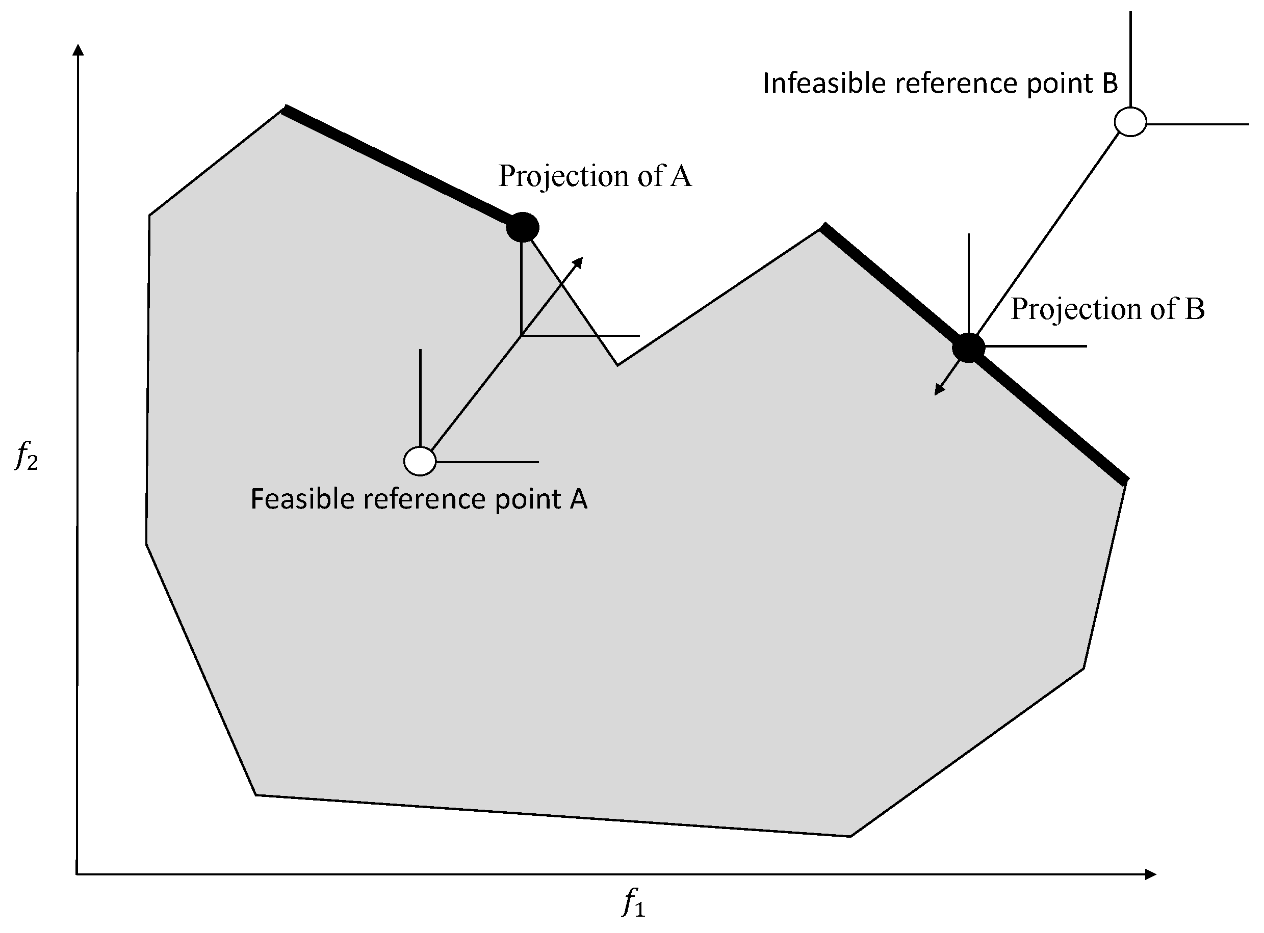
4.4. Reference Point Method (Wierzbicki, 1980) [20]
The Reference Point method [
20] asks the DM to provide aspiration levels for the objectives. The aspiration point is then projected to the non-dominated frontier. Note that it does not matter whether the aspiration point provided by the DM is feasible or not. In the projection, Wierzbicki used the so-called Achievement Scalarizing Function (ASF), which was minimized as:
where
is a set of weights,
is a small number, and
is the vector of aspiration levels. Note that when
, the indifference contours being optimized are orthogonal (90 degree angle); when
, the indifference contours being optimized form an angle between 90 and 180 degrees. Once the non-dominated projection of the aspiration levels is found, the method asks the DM to update the aspiration levels. The method stops when the DM is satisfied with the solution. In contrast with the GDF and ZW methods, no assumptions of
U are made.
4.5. Reference Direction Approach (Korhonen and Laakso, 1986) [46]
Instead of projecting a single reference point using Wierzbicki’s ASF, Korhonen and Laakso [
46] suggested projecting multiple directions to the efficient frontier. The projection was determined by solving the following parametric program:
where
is a set of weights,
is any vector in the criterion space, and
is a reference direction, with
being an aspiration level or a reference goal in the spirit of Wierzbicki’s reference point approach. When the parameter
t in the above problem is varied from zero to infinity, an efficient curve emanating from point
is obtained.
The interface of the reference direction method is similar to the GDF method. When the DM has identified the most preferred solution along the projection, then they are asked to revise their aspiration point, and the process is repeated. An extension and application of the reference direction approach on multi-objective quadratic linear programming can be found in [
50].
4.6. Pareto Race (Korhonen and Wallenius, 1988) [47]
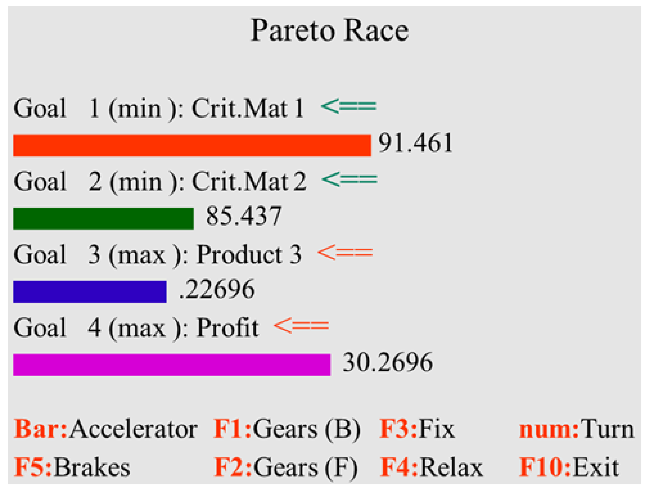
Pareto Race [
47] is a visual, dynamic search procedure for exploring the non-dominated frontier of a multi-objective LP problem. It is based on the idea of projecting reference directions on the efficient frontier. However, no aspiration levels are elicited from the DM. Instead, if the DM wants to improve the value of a certain objective, they press the number key (one or more times, depending on the relative desired improvement in that objective) of the corresponding objective.
There is an analogy to driving an automobile (on the efficient frontier). The user sees the objective function values on a display in numeric form and as bar graphs as they travel along the non-dominated frontier. Keyboard controls include accelerator, gears, breaks, and a steering mechanism. Technically, two parameters are used to control the motion: the reference direction (direction) and step size (speed).
Figure 8 shows the interactive dashboard used in the Pareto Race approach.
5. EMO Introduction and History
An evolutionary algorithm is a general population-based optimization algorithm which uses a mechanism inspired by biological evolution, i.e., selection, crossover, mutation, and replacement. The common underlying idea behind an evolutionary technique is that, for a given population of individuals, the environmental pressure causes natural selection, which leads to a rise in fitness of the population. A comprehensive discussion of the principles of an evolutionary algorithm can be found in [
51,
52,
53,
54,
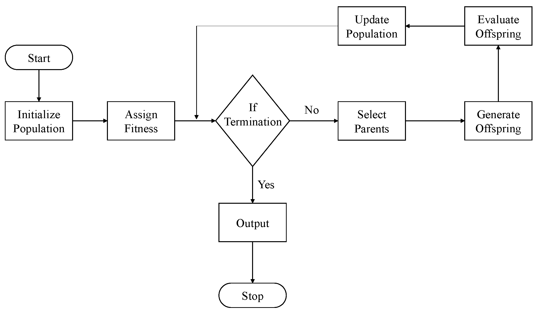
55]. In contrast to classical algorithms, which iterate from one solution point to the other until termination, an evolutionary algorithm works with a population of solution points. Each iteration of an evolutionary algorithm results in an update of the previous population by eliminating inferior solution points and including the superior ones. In the terminology of evolutionary algorithms, an iteration is commonly referred to as a generation and a solution point as an individual. A pseudo-code for a general genetic algorithm, which is a type of evolutionary algorithm, is provided below:
Step 1: Create a random initial population (i.e., a set of solution points in the decision space).
Step 2: Evaluate the individuals (i.e., the solution points) in the population with respect to objective(s) and constraints, if present, and assign fitness (i.e., quality measure).
Step 3: Repeat the generations (i.e., iterations of the evolutionary algorithm) until termination.
Substep 1: Select the fitter individuals (referred to as parents) from the population for reproduction (i.e., producing new solution points through genetic operators of crossover and mutation).
Substep 2: Produce new individuals (referred to as offspring) through crossover and mutation operators.
Substep 3: Evaluate the new individuals and assign fitness.
Substep 4: Replace the low-fitness individuals in the population with high-fitness individuals that may have been generated through crossover and mutation.
Step 4: Report the highest fitness individual as the output.
Along with the pseudo-code presented above, a flowchart for a general evolutionary algorithm is presented in
Figure 9. In evolutionary algorithms, to begin with, a pool of individuals is generated by randomly creating points in the search space, which is called the population. Each individual in the population is evaluated on objective(s) and constraints (if any) and is assigned a fitness. For instance, while solving a single-objective maximization problem, a solution point with a higher function value is better than a solution point with lower function value when both solutions are feasible. Therefore, in such cases, the individual with higher function value is assigned a higher fitness. While comparing two infeasible solutions, the solution with a smaller constraint violation is often assigned a higher fitness as compared with the solution with larger constraint violation. In the presence of multiple constraints, the constraint violation for a particular point is defined as the sum of violation of those constraints that are infeasible with respect to that point. While comparing a feasible solution against an infeasible solution, a feasible solution is often assigned a higher fitness as compared with the infeasible solution. There can, of course, be other ways to assign fitness. For an unconstrained maximization problem, the function value itself can be treated as the fitness value and, for an unconstrained minimization problem negative of the function value, may serve the purpose of fitness. In all such cases, the algorithm searches for a higher fitness solution.
In a multi-objective context, the requirement is to produce a set of solutions that approximate the Pareto-optimal front. Fitness assignment based on constraint violation can be performed in the multi-objective case in a similar manner as the single-objective case. Moreover, a feasible solution point which dominates another feasible solution point can be assigned a higher fitness. However, fitness assignment for two solutions that are non-dominated with respect to each other is tricky. In such cases, algorithms often consider a measure of diversity or crowdedness [
4] in the objective space to assign fitness and prefer one solution over the other. The measure for crowdedness prefers solutions that are isolated over solutions that are in crowded regions to enhance diversity in the population and to obtain a “well-spread” set of solutions approximating the Pareto-optimal front. A multi-objective evolutionary procedure, therefore, assigns fitness to each of the solution points based on their superiority over other solution points in terms of constraints, dominance, and diversity in the objective space. Different algorithms use different quality functions to assign fitness to an individual in a population. Once an initial population is generated and the fitness is assigned, a few of the better candidates from the population are chosen as parents. Crossover and mutation are performed to generate new solutions. Crossover is an operator applied to two or more selected individuals and results in one or more new individuals. Mutation is applied to a single individual and results in one new individual. Executing crossover and mutation lead to offspring that compete, based on their fitness, with the individuals in the population, for a place in the next generation. An iteration of this process often leads to a rise in the average fitness of the population and, over iterations, helps the algorithm converge towards the optimum in a single-objective case and towards the Pareto-optimal front in a multi-objective case.
Using the described evolutionary framework, a number of algorithms have been developed which successfully solve a variety of optimization problems. Their strength is particularly observable in handling two- to three-objective optimization problems and generating the entire Pareto-front. The aim of an EMO algorithm is to produce solutions which are (ideally) Pareto-optimal and uniformly distributed over the entire Pareto-front, so that a complete representation is provided. In the domain of EMO algorithms, these aims are commonly referred to as convergence and diversity.
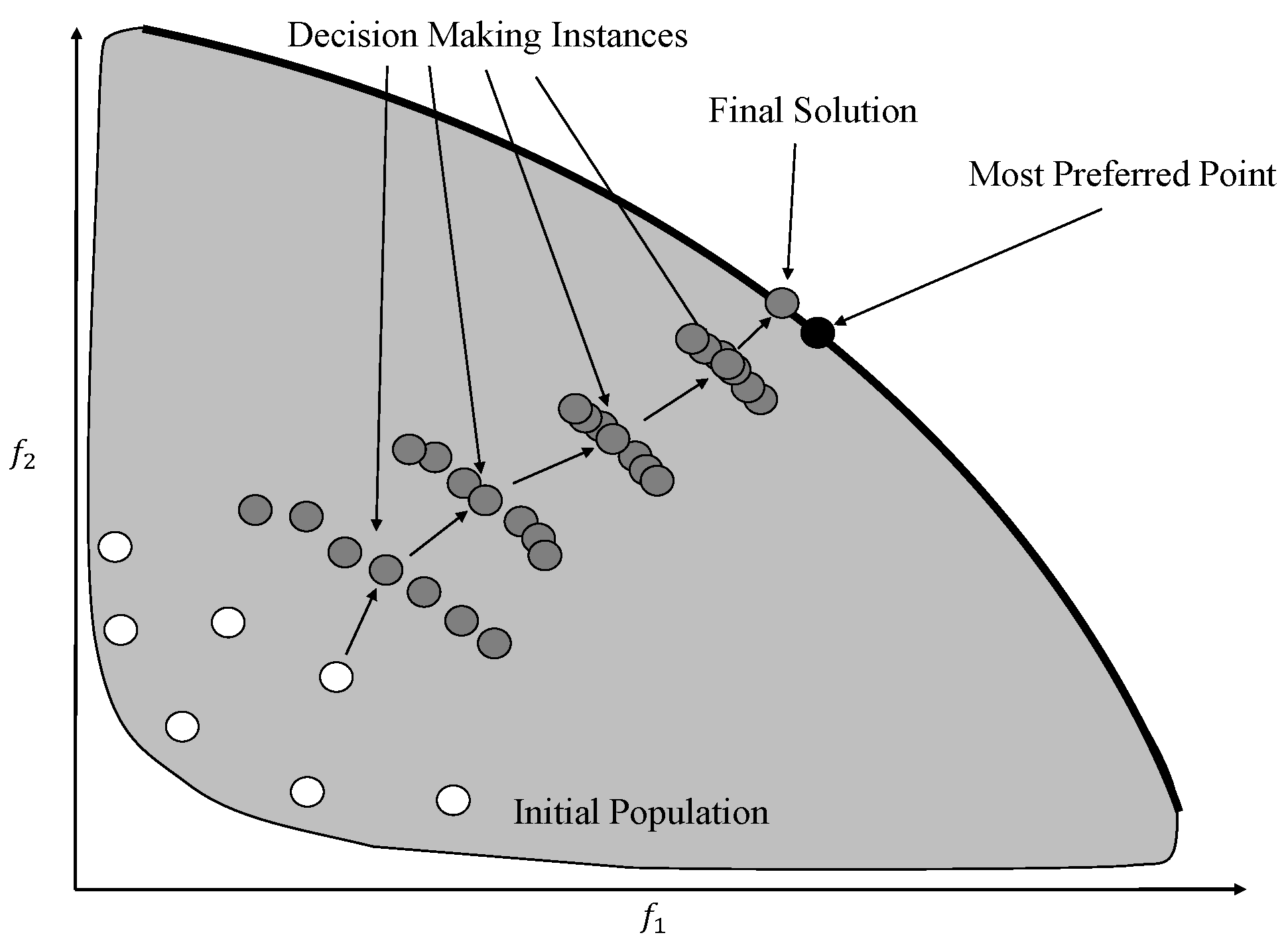
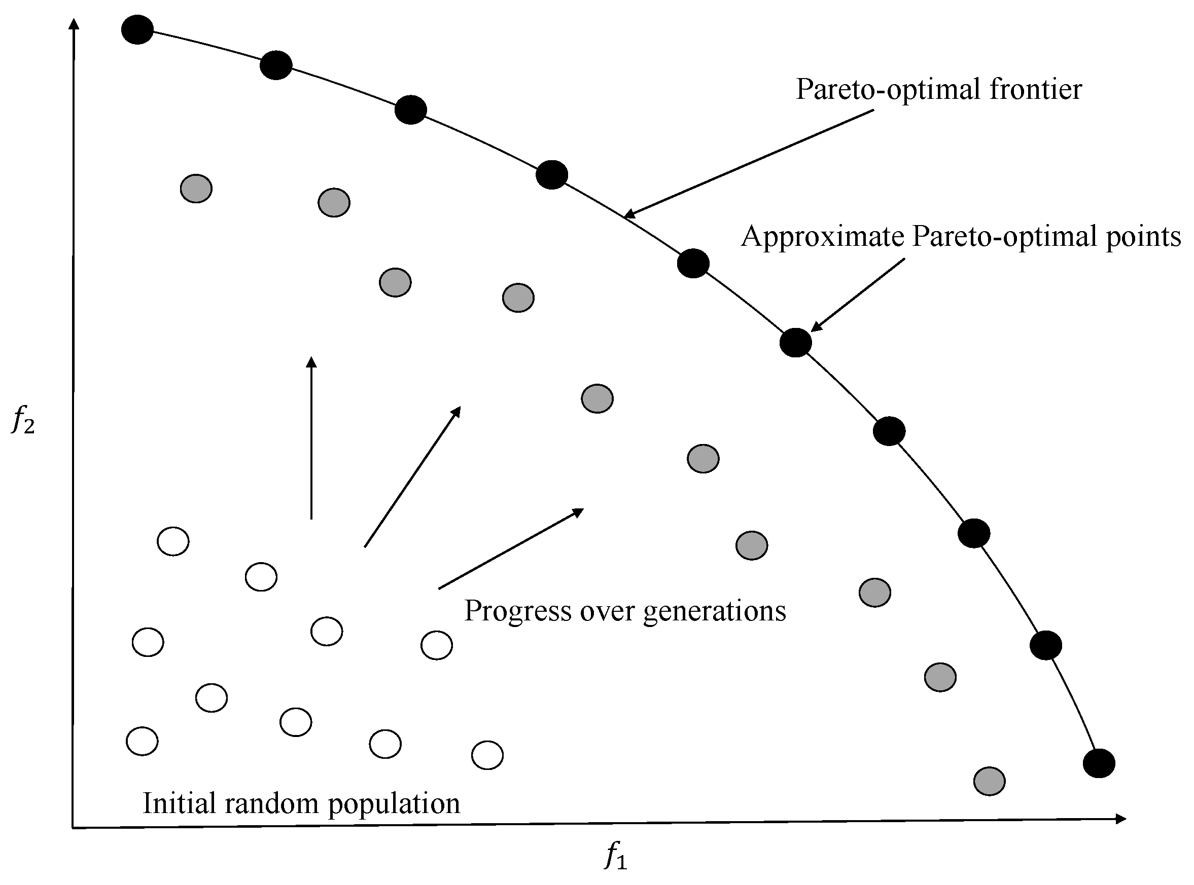
Figure 10 shows the working of a typical EMO algorithm that starts with a random initial population and aims to converge to the efficient frontier with a diverse set of solutions. The researchers in the EMO community have so far regarded an
a posteriori approach to be an ideal approach where a representative set of Pareto-optimal solutions are found and then a DM is invited to select the most preferred point. The assertion is that only a DM who is well-informed is in a position to take a right decision. A common belief is that decision making should be based on complete knowledge of the available alternatives; current research in the field of EMO algorithms has taken inspiration from this belief. Though the belief is true to a certain extent, there are inherent difficulties associated with producing the entire set of alternatives and performing decision making thereafter, which many a time renders the approach ineffective.
The EMO approaches can be divided into three broad categories based on the idea that they use to achieve convergence and diversity. The categories are:
While Pareto-based approaches have been popular for solving two- or three-objective test problems, their efficiency deteriorates on problems with a higher number of objectives. Many of these methods are based on the approach of non-dominated sorting of the population as the primary driver. In problems with a large number of objectives, most of the solutions generated by these approaches are non-dominated in the comparison set leading to deterioration in progress towards the Pareto-frontier. Indicator-based approaches attempt to optimize a particular indicator that accounts for both convergence and diversity but did not become popular because of high computational costs involved in computing the indicator metric (for example, Hypervolume or Inverted Generational Distance) in many-objective problems. Despite these issues, both Pareto-based and indicator-based methods still hold promise, as non-dominated sorting in Pareto-based approaches is one of the fundamental ideas for partial ordering that cannot be ignored; similarly, faster computation of indicator metrics would make the indicator-based approaches competitive.
An alternative to Pareto-based approaches and indicator-based approaches are decomposition-based approaches, which have been effective in handling a larger number of objectives by decomposing the original problem into a set of subproblems, either multiple single-objective problems or multiple simplified multi-objective problems. These multiple problems are solved simultaneously in a collaborative manner and lead to better convergence and diversity, as the convergence is guaranteed by ensuring that each subproblem is properly optimized, and diversity is guaranteed by implicitly distributing the subproblems in an even manner. Interestingly, the decomposition-based methods utilize MCDM approaches while decomposing the multi-objective problems into subproblems. For instance, a distributed set of reference directions from the ideal point (or sometimes from the nadir point) towards the Pareto-front would lead to a well-distributed set of Pareto-optimal solutions if the front is uniform in shape. The methods that rely on decomposition solve these subproblems in a parallel manner and differ mostly on the basis of how the subproblems are created, how information between subproblems is shared during the generations, and how the subproblems may adapt during intermediate generations. However, note that if one considers a 10-objective problem, with a discretization of 10 along each objective, one would need
points to approximate the frontier. Moreover, even if the points are produced by a computationally efficient algorithm, the decision-making challenge still remains. If the Pareto-front is not found with sufficient discretization, the DM may expect the method to explore additional solutions. For the purpose of evaluating the EMO approaches, a large body of literature exists on test problem toolkits [
62,
63,
64,
65] and performance assessment metrics [
66,
67,
68,
69,
70] that allow the developers to compare the performance of various algorithms.
6. Hybrid Methods
In this section, we focus on hybrid approaches that incorporate decision making within EMO. As already highlighted, the aim of the EMO algorithms is to find a diverse set of solutions close to the Pareto-optimal front, and the DM is then expected to choose the most preferred point from the objective space. However, approximating the entire Pareto-optimal front with a set of points is not always easy and may not serve the purpose, especially in the context of problems with a large number of objectives. To alleviate these problems associated with
a posteriori EMO approaches, some EMO researchers taking cues from their MCDM counterparts have attempted an
a priori approach, where a small set of Pareto-optimal points in the region of interest to the DM is targeted. As soon as the region of interest becomes smaller, certain problems associated with the high dimensionality of the problem in the objective space gets alleviated. Greenwood et al. [
30] used an evolutionary approach to optimize a linear value function obtained from the DM through ranking of a few alternatives. In this method, the preference information is employed before optimization, and therefore this qualifies as an
a priori method. Other studies in this direction are the cone-dominance-based EMO [
71], biased-niching-based EMO [
27], the light beam approach based EMO [
35], and reference-point-based EMO approaches [
28,
29].
In [
71], the authors modify the dominance principle based on interactions with the DM. For every pair of objectives, the DM specifies maximally acceptable trade-offs, i.e., what is the improvement of one unit in one objective (say
) worth in terms of degradation of another objective (say
). If the degradation is worth at most
in
when
improves by unity, and at most
in
when
improves by unity, then the dominance scheme
is modified as follows with a strict inequality in at least one case:
Incorporating the above principle in an EMO is straightforward, as one can simply replace objectives
and
with
and
, respectively, where
and
are defined below, and solve the problem with the standard dominance principle.
The approach can be incorporated in any EMO and does not lead to any increase in complexity.
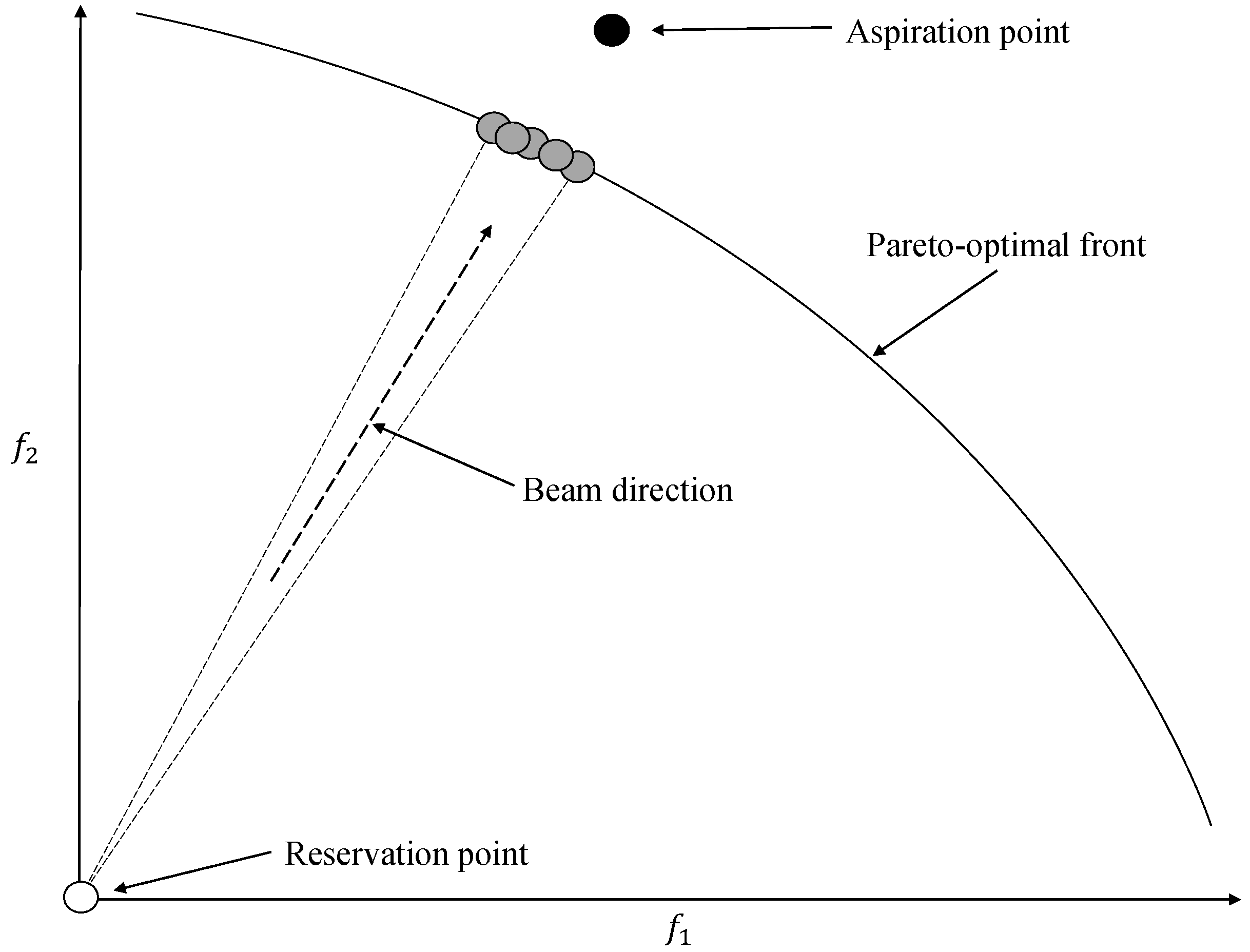
Figure 11 and
Figure 12 indicate the working of the light beam approach based EMO [
35] and the reference-direction-based EMO [
28,
29] approaches, respectively. In their study, Jaskiewicz and Branke [
40] showed that it is difficult for an EMO algorithm alone to find a good spread of solutions in five- to ten-objective problems, and when solutions around the most preferred point are targeted, the hybrid approaches are able to find satisfactory solutions.
Preference-based EMO algorithms can differ from each other based on the following aspects:
Stage at which preference is incorporated;
Manner in which preference information is elicited;
Type of preference modeling performed;
Integration of preference model with EMO search;
Choice of the EMO, i.e., Pareto-based, indicator-based or decomposition-based.
Apart from a priori and a posteriori approaches, a more seamless and effective way to incorporate DMs’ preferences in the EMO would be to collect and incorporate preferences at the intermediate generations of the EMO algorithm to guide the search towards the most preferred point. Such an approach is commonly referred to as a progressively interactive EMO approach. We discuss, in detail, some of the progressively interactive techniques studied in the literature.
6.1. Phelps and Köksalan (2003) [38]
Phelps and Köksalan [
38] presented one of the first hybrid approaches, where they optimized a linearly weighted utility function during the iterations of an evolutionary algorithm. The decision maker makes a number of binary comparisons that leads to the weights of the utility function. For a given parameter
t and ideal point
, the authors solve the following optimization problem to obtain the weights
.
The above problem is an LP that leads to
used in calculating the fitness of each point using the following utility function:
The preference from the DM is taken initially or during the execution of the algorithm to modify the fitness function. The authors considered linear utility functions in their study.
To incorporate the properties of an implicit quasi-concave utility function into an EMO, Fowler et al. [
39] developed an interactive EMO approach using convex preference cones. They used feasibility, dominance, and preference cones to order the population members and used that information for fitness calculation. They tested their algorithm on multi-dimensional (up to four dimensions) knapsack problems using a similar interactive genetic algorithm framework to that of Phelps and Köksalan [
38]. Jaszkiewicz [
40] constructed an achievement scalarizing function using random weights. The random weights are preferred if the scalarizing function generated conforms to the preference information provided by the DM. The EMO search is then guided by the scalarizing function generated with random weights.
6.2. Branke, Greco, Słowiński, and Zielniewicz (2009) [41]
Branke et al. [
41] implemented the GRIP [
72] methodology, in which the DM-provided pairwise information is used to find all possible compatible additive value functions (not necessarily linear). A preference-based dominance relationship and a preference-based diversity preserving operator is used in an EMO to find new solutions for the next few generations. In their approach, they make pairwise comparisons after every few generations in order to develop the preference structure. It is also possible for the DM to specify the intensities of preference. The authors use robust ordinal regression on information obtained through interaction with the DM to determine the set of all compatible value functions. Thereafter, the EMO procedure performs a parallel search for all non-dominated solutions that are preferred with respect to the compatible value functions. The authors demonstrated their procedure on a two-objective test problem. The study was later extended to solve up to five-objective test problems in [
73]. The study takes a robustness approach to avoid arbitrary selection of a value function, which makes it different from most of the other studies that determine the single most discriminating value function. The use of preference information in a robust manner in EMO is a significant contribution of this study. Other recent studies that use a set of instances of the preference model compatible with the DM’s preference information are [
74,
75]. These studies generate multiple instances of the preference model using Monte Carlo simulation and utilize the instances as search directions in a decomposition-based EMO approach.
6.3. Deb, Sinha, Korhonen, and Wallenius (2010) [42]
Based on earlier interactive MCDM approaches [
76,
77], this paper proposes a preference-based EMO to guide a DM to the most preferred solution by creating non-linear value functions in the intermediate generations of the algorithm. The approach accepts preference information in the form of complete or partial ranking, i.e., the DM may prefer one solution over the other or the DM may be indifferent between two solutions. The authors do not consider the situation where the DM is unable to compare two solutions. Through an extensive computational study on two- to five-objective problems, the authors evaluated the performance of their approach when the DM interacts less/more frequently with the EMO approach, as well as the impact on the quality of the solution produced when the DM provides erroneous preference information. The approach utilized the approximated value function in an innovative manner by partitioning the objective space into two areas using the value function. They also utilized the value function for performing local search and termination of the method.
In this paper, the authors fit a polynomial value function with the following structure for two objectives.
For a higher number of objectives, they use a higher-order polynomial function of the following kind:
where
for all
i, and
for
and for all
i. The value function is fitted by solving the following optimization problem with respect to the value function parameters when preference information is available:
A look into the above optimization problem reveals that it attempts to find a value function for which the minimum difference in the value function values between the ordered pairs of points is maximum. At the same time, it also ensures that the difference in the value function values for a pair of indifferent points is smaller than a threshold that is proposed to be
.
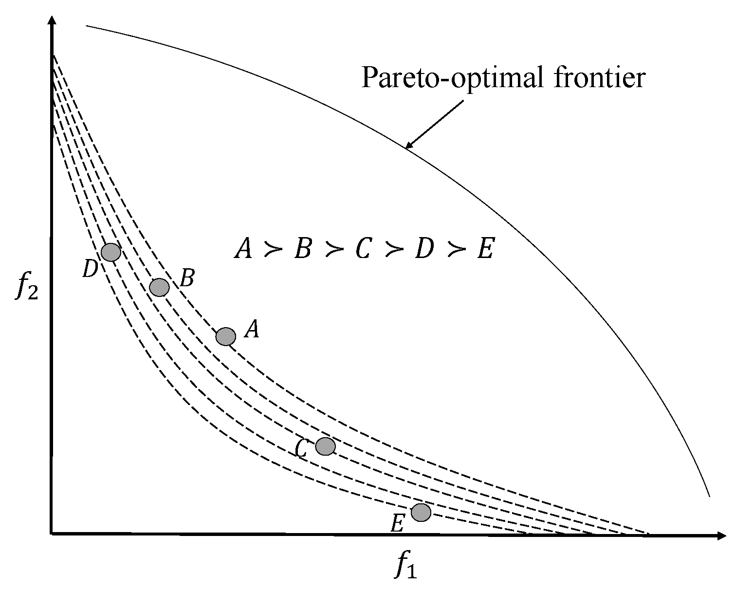
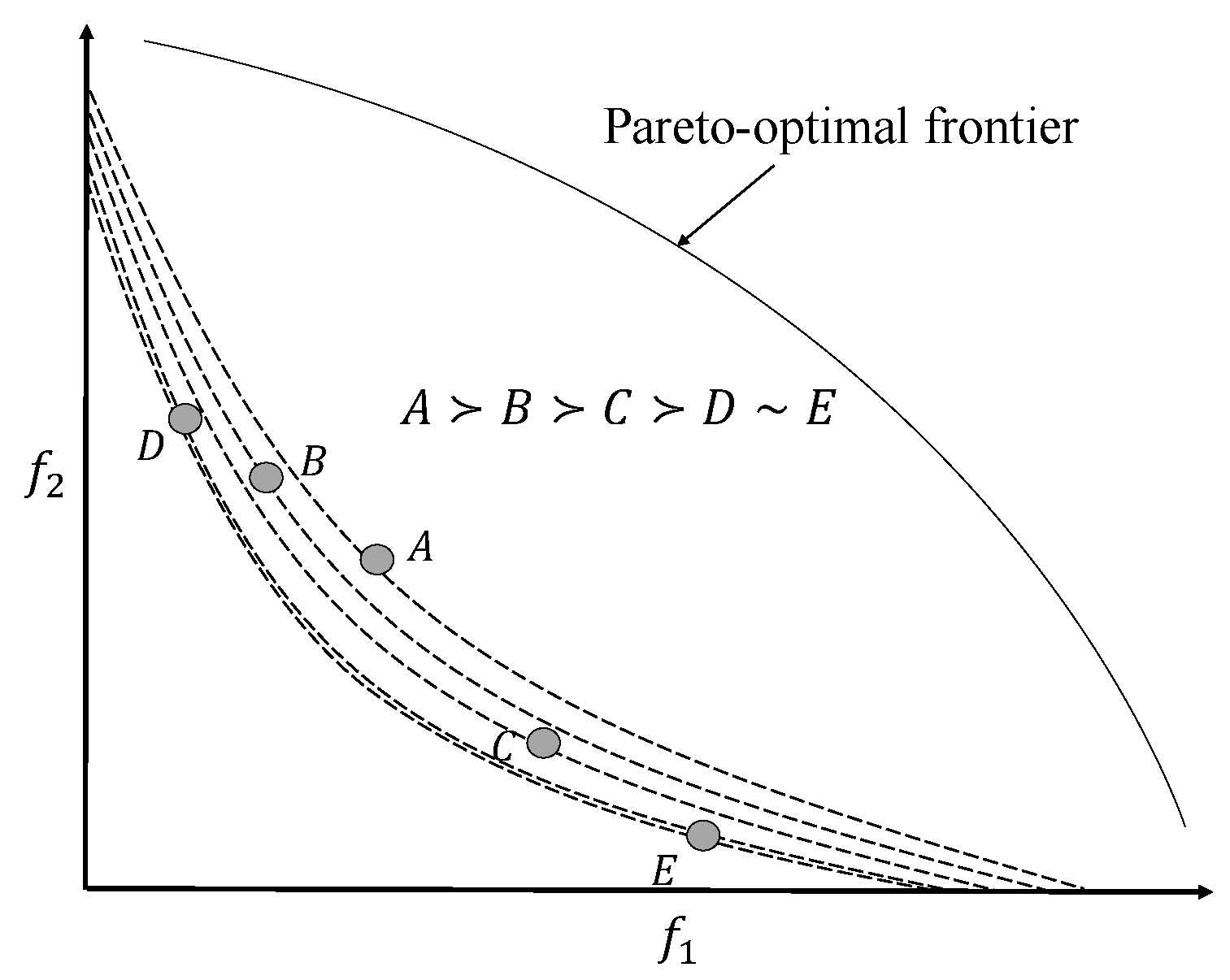
Figure 13 and
Figure 14 show how the preference structure is captured using the value function when points have a complete or a partial order, respectively. An extension of this study suggested a generalized polynomial value function [
78]; however, any attempt to fit a very complex value function to user preference is not always advisable. Unless there are errors or conflicts in preference information, the preference structure in a region can often be captured using relatively simple value functions.
6.4. Sinha, Deb, Korhonen, and Wallenius (2014) [43]
In this study, Sinha et al. [
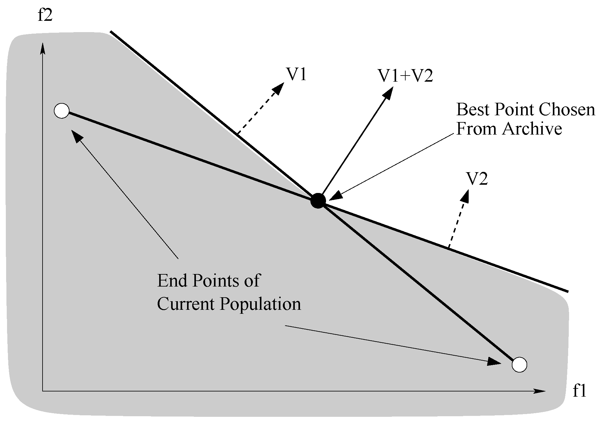
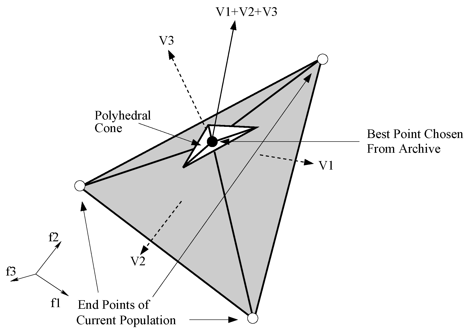
43] generate the most preferred solution on the Pareto-optimal frontier in a fixed budget of decision-making calls. Most of the earlier hybrid approaches did not assume that the DM will be available for providing preferences only for a fixed number of times. In fact, in most of the procedures, there is no control on the number of DM calls, or the DM calls are not utilized effectively. The assumption in most of the interactive approaches is that the DM would be available for as many interactions as desired by the method until a satisfactory solution is found; however, this is not a wise assumption to make. The approach discussed in this section attempts to address this concern by solving the problem in a fixed number of interactions with the DM. The study also deviated from constructing value functions and, instead, suggested constructing polyhedral cones heuristically to guide the EMO. The authors tested their approach on two- to five-objective test problems and studied the impact of increasing or decreasing the budget of DM calls on the performance of the algorithm in getting close to the most preferred point.
The algorithm requires the ideal point at start. Once the ideal point is known, the initial random population is created, and the point in the initial population closest to the ideal point is chosen. Let the distance be denoted as . This distance is divided into certain equal parts (say ) based on the budget of DM calls available. Thereafter, the EMO run starts, and preference from the DM is elicited only after a progress of has been made. During the progress, the algorithm stores all non-dominated solutions produced in an archive set, and preference from the DM is taken in terms of the most preferred point from the archive set.
The method heuristically constructs a polyhedral cone using the most preferred solution suggested by the DM from the archive set and the end points along each of the objectives. For a
p-objective problem, a polyhedral cone is formed using
points.
Figure 15 and
Figure 16 show the construction of cones in two and three dimensions. Once the polyhedral cone is determined, it provides an idea for a search direction. The normal unit vectors (
) of all the
p hyperplanes can be summed up to obtain a heuristic search direction (
), which is used in the algorithm for the purpose of local search.
As an extension, a mathematically driven preference-cone-based approach was later proposed in [
79], where the user’s preferences were assumed to follow an unknown quasi-concave and increasing value function. In addition to considering the preference cones as a tool for eliminating non-preferred solutions, the authors also presented how the cones could be leveraged in approximating the steepest ascent direction to guide an evolutionary algorithm. A merit function is proposed that the authors use for fitness calculations in the algorithm. In addition to test problems, a mixed-integer facility location problem was solved in the later study.
7. Interaction Styles, Behavioral Considerations, and Future Work
Given that preferences can be elicited in a number of ways, developers of a specific method normally think that the interaction style embedded in their approach is the best. However, we need more research to answer what kind of cognitive load is caused by the interaction style (preference elicitation) and which interaction style leads closer to the true most preferred solution. An interesting approach is to use neuro-physiological measurement instruments to measure the DM’s cognitive and emotional load. Scholars in the 1970s pioneered the idea of interactively solving multi-objective problems, which was remarkable considering the state of the art of computer technology in the early to mid 1970s. No personal computers, nor computer graphics capabilities, were available before the early 1980s. Scholars had to access the main frame computer via teletypes (time sharing). Their contribution was not the development of the concept of efficient or Pareto-optimal solution, rather, it was Pareto who introduced the ideas of non-dominance. However, the scholars during the period made it possible to explore or move around the non-dominated frontier in an effective way. Problems studied were largely limited to LP framework (convex and compact feasible sets).
With computation becoming faster, newer applications arising in practice, and numerical or computational techniques for more general classes of problems being developed, researchers started looking beyond LPs. However, the decision-making difficulties did not receive the attention they deserved. For instance, there has been only limited effort in trying to solve multi-objective problems in a fixed number of interactions with the DM [
43,
80]. The decision-making calls are often assumed to be an unlimited resource, with the expectation that the DM is available for a large number of interactions.
Termination criterion for methods involving human–machine interaction is a challenge. Optimization methods may terminate based on gradient-based criterion, Karush–Kuhn–Tucker-based criterion, or improvement-based criterion. However, with the DM interacting with the method, it is difficult to terminate the process, as one does not know in advance the proximity of the current best solution for the DM to the true most preferred solution. Effort is also required on visualization techniques to reduce the burden on the DM during the decision-making process. Many of the visualization techniques focus on commonly used descriptive approaches, such as scatter plots, bar charts, value plots, etc. However, very few of the techniques offer an immersive experience to the DM, where the DM can easily navigate in the search space, understand trade-offs, possible improvements, and then make a decision. A comprehensive review of visualization-based approaches can be found in [
81,
82].
Other challenges in the decision-making context which have led to difficulties in preference modeling are as follows:
DM providing erroneous preferences;
DM providing conflicting or inconsistent preferences;
DM preference structure changing in different regions of the objective space;
DM preference structure changing as a function of learning;
DM becoming biased (anchored) based on the initial set of options presented;
DM unable to compare two options in terms of either dominance or indifference.
Significant effort is still required towards developing decision-making and search techniques that are robust to the above mentioned issues.


