1. Introduction
Practical problems often require expensive simulation of accurate high-fidelity models. To get close to the optimum of these models, most multiobjective optimization algorithms need to compute a large number of solution evaluations. However, in practice, only a handful of solution evaluations are allowed due to the overall time constraint available to solve such problems. Researchers usually resort to surrogate models or metamodels constructed from a few high-fidelity solution evaluations to replace computationally expensive models to drive an optimization task [
1,
2,
3]. For example, Gaussian process model, Kriging, or response surface method is commonly used. The Kriging method is of particular interest, since it is able to provide an approximated function as well as an estimate of uncertainty of the prediction of the function [
4].
In extending the metamodeling concept to multiobjective optimization problems, an obvious issue is that multiple objective and constraint functions are required to be metamodeled before proceeding with the optimization algorithm. Despite this challenge of multiple metamodeling efforts, a good number of studies have been made to solve computationally expensive multiobjective optimization problems using metamodeling based evolutionary algorithms [
5,
6,
7,
8,
9,
10]. However, most of these studies ignored constraints and extending an unconstrained optimization algorithm to constrained optimization is not trivial [
11]. In any case, the structure of most of these methods is as follows. Starting an initial archive of solutions obtained by an usual Latin-hypercube sampling, a metamodel for each objective and constraint function is built independently [
12,
13]. Then, in an
epoch–one cycle of metamodel development and their use to obtain a set of
in-fill solutions, an evolutionary multiobjective optimization (EMO) algorithm is used to optimize the metamodeled objectives and constraints to find one or more in-fill points. Thereafter, the in-fill points are evaluated using high-fidelity models and saved into the archive. Next, new metamodels are built using the augmented archive members and the procedure is repeated in several epochs until the allocated number of solution evaluations is consumed [
5,
14,
15,
16,
17,
18,
19]. Many computationally expensive optimization problems involve noisy high-fidelity simulation models. Noise can come from inputs, stochastic processes of the simulation, or the output measurements. In this paper, we do not explicitly discuss the effect of noise in handling metamodeling problems, but we recognize that this is an important matter in solving practical problems.
In a recent taxonomy study [
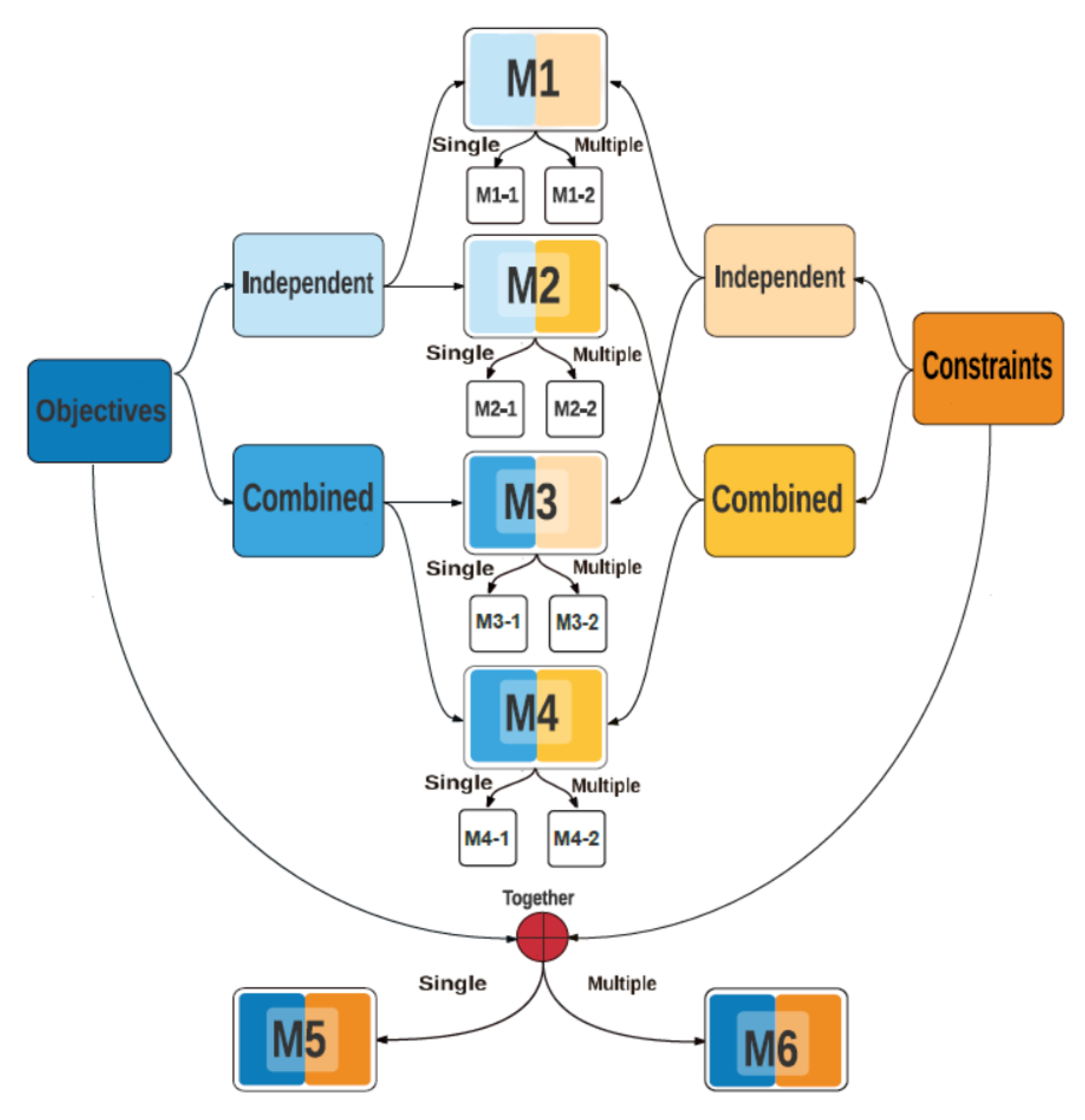
20], authors have categorized different plausible multiobjective metamodeling approaches into 10 frameworks, of which the above-described popular method falls within the first two frameworks—M1-1 or M1-2, depending on whether a single or multiple nondominated in-fill solutions are found in each epoch. The other eight frameworks were not straightforward from a point of view extending single-objective metamodeling approaches to multiobjective optimization and hence were not explored in the past. Moreover, the final two frameworks (M5 and M6) attempt to metamodel an EMO algorithm’s implicit overall fitness (or selection) function directly, instead of metamodeling an aggregate or individual objective and constraint functions. There is an advantage of formulating a taxonomy, so that any foreseeable future metamodeling method can also be categorized to fall within one of the 10 frameworks. Moreover, the taxonomy also provides new insights to other currently unexplored ways of handling metamodels within a multiobjective optimization algorithm.
So far, each framework has been applied alone in one complete optimization run to solve a problem, but in a recent study [
21], a manual switching of one framework to another after 50% of allocated solution evaluations has produced improved results. An optimization process goes through different features of the multiobjective landscape and it is natural that a different metamodeling framework may be efficient at different phases of a run. These studies are the genesis of this current study, in which we propose an adaptive switching based metamodeling (ASM) approach, which automatically finds one of the 10 best-performing frameworks at the end of each epoch after a detailed statistical study, thereby establishing self-adaptive and efficient overall metamodeling based optimization approach.
In the remainder of the paper,
Section 2 briefly describes a summary of recent related works.
Section 3 provides a brief description of each of 10 metamodeling frameworks for multiobjective optimization. The proposed ASM approach is described in
Section 4. Our extensive results on unconstrained and constrained test problems for each framework alone and the ASM approach are presented in
Section 5. A comparative study of the ASM approach with three recent existing algorithms is presented in
Section 5.5. We summarize our study of the switching framework based surrogate-assisted optimization with future research directions in
Section 6.
2. Past Methods of Metamodeling for Multiobjective Optimization
We consider the following original multi- or many-objective optimization problem (
P), involving
n real-valued variables (
),
J inequality constraints (
) (equality constraints, if any, are assumed to be converted to two inequality constraints), and
M objective functions (
):
In this study, we assume that all objective and constraint functions are computationally expensive to compute and that they need to be computed independent to each other for every new solution . To distinguish from the original functions, the respective metamodeled function is represented with a “tilde ” (such as, or ). The resulting metamodeled problem is denoted here as , which is formed with developed metamodels of individual objective and constraints or their aggregates. In-fill solutions are defined as optimal solutions of problem . It is assumed here that constructing the metamodels and their comparisons among each other consume comparatively much less time than evaluating objective and constraints exactly, hence, if the metamodels are close to the original functions, the process can end up with a huge savings in computational time without much sacrifice in solution accuracy. Naturally, in-fill solutions (obtained from metamodels) need to be evaluated using original objective and constraints (termed here as “high-fidelity” evaluations) and can be used to refine the metamodels for their subsequent use within the overall optimization approach.
A number of efficient metamodeling frameworks have been proposed recently for multiobjective optimization [
10,
22,
23,
24,
25,
26,
27,
28], including a parallel implementation concept [
29]. These frameworks use different metamodeling methods to approximate objective and constraint functions, such as radial basis functions (RBFs), Kriging, Bayesian neural network, support vector regression, and others [
30]. Most of these methods proposed a separate metamodel for each objective and constraint function, akin to our framework M1. Another study have used multiple spatially distributed surrogate models for multiobjective optimization [
31]. It is clear that this requires a lot of metamodeling efforts and metamodeling errors from different models can accrue and make the overall optimization to be highly error-prone. As will be clear later, these methods will fall under our M1-2 framework.
Zhang et al. [
14] proposed the MOEA/D-EGO algorithm which metamodeled each objective function independently. They constructed multiple expected global optimization (EGO) functions for multiple reference lines of the MOEA/D approach to find a number of trade-off solutions in each optimization task. No constraint handling procedure was suggested. Thus, this method falls under our M1-2 framework.
Chugh et al. [
23] proposed a surrogate-assisted adaptive reference vectors guided evolutionary algorithm (K-RVEA) for computationally expensive optimization problems with more than three objectives. Since all objectives and constraints are metamodeled separately, this method also falls under our M1-2 framework. While no constraint handling was proposed with the original study, a later version included constraint handling [
32].
Zhao et al. [
24] classified the sample data into clusters based on their similarities in the variable space. Then, a local metamodel was built for each cluster of the sample data. A global metamodel is then built using these local metamodels considering their contributions in different regions of the variable space. Due to the construction and optimization of multiple metamodels, one for each cluster, this method belongs to our M-3 framework. The use of a global metamodel by combining all local cluster-wise metamodels qualify this method under the M3-2 framework. No constraint handling method is suggested.
Bhattacharjee et al. [
25] used an independent metamodel for each objective and constraint using different metamodeling methods: RBF, Kriging, first and second-order response surface models, and multilayer perceptrons. NSGA-II method is used to optimized metamodeled version of the problem. Clearly, this method falls under our M1-2 category.
Wang et al. [
26] used independent metamodeling of objectives but combined them using a weight-sum approach proposed an ensemble-based model management strategy for surrogate-assisted evolutionary algorithm. Thus, due to modeling a combined objective function, this method falls under our M3-1 framework. A global model management strategy inspired from committee-based active learning (CAL) was developed, searching for the best and most uncertain solutions according to a surrogate ensemble using a particle swarm optimization (PSO) algorithm. In addition, a local surrogate model is built around the best solution obtained so far. Then, a PSO algorithm searches on the local surrogate to find its optimum and evaluates it. The evolutionary search using the global model management strategy switches to the local search once no further improvement can be observed and vice versa.
Pan et al. [
33] proposed a classification based surrogate-assisted evolutionary algorithm (CSEA) for solving unconstrained optimization problems by using an artificial neural network (ANN) as a surrogate model. The surrogate model aims to learn the dominance relationship between the candidate solutions and a set of selected reference solutions. Due to a single metamodel to find the dominance structure involving all objective functions, this algorithm falls under our M3-2 framework.
Deepti et al. [
34] suggested a reduced and simplified model of each objective function in order to reduce the computational efforts.
Recent studies on nonevolutionary optimization methods for multiobjective optimization using trust-region method [
35,
36] and using decomposition methods [
37] are proposed as well.
A recent study [
38] reviewed multiobjective metamodeling approaches and suggested a taxonomy of the existing methods based on whether the surrogate assisted values match well the original function values. Three broad categories were suggested: (i) algorithms that do not use any feedback from the original function values, (ii) algorithms that use a fixed number of feedback, and (iii) algorithms that adaptively decide which metamodeled solutions must be checked with the original function values. This extensive review reported that most existing metamodeling approaches used a specific EMO algorithm—NSGA-II [
39]. While a check on the accuracy of a metamodel is important for its subsequent use, this is true for both single and multiobjective optimization and no specific issues related to multiobjective optmization were discussed in the review paper.
Besides the algorithmic developments, a number of studies have applied metamodeling methods to practical problems with a limited budget of solution evaluations [
40,
41,
42,
43,
44,
45,
46,
47], some restricting to a few hundreds [
48].
Despite all the above all-around developments, the ideas that most distinguish surrogate modeling in multiobjective optimization from their single-objective counterparts were not addressed well. They are (i) how to fundamentally handle multiple objectives and constraints either through a separate modeling of each or in an aggregated fashion? and (ii) how to make use of the best of different multiple surrogate modeling approaches adaptively within an algorithm? In 2016, Rayan et al. [
5] have proposed a taxonomy in which 10 metamodeling frameworks were proposed to address the first question. This paper addresses the second question in a comprehensive manner using the proposed 10 metamodeling frameworks using an ensemble method.
Ensemble methods have been used in surrogate-assisted optimization for solving expensive problems [
49,
50,
51,
52,
53], but in most of these methods, an ensemble of different metamodeling methods, such as RBF, Kriging, response surfaces, are considered to choose a single suitable method. While such studies are important, depending on the use of objectives and constraints, each such method will fall in one of the first eight frameworks presented in this paper. No effort is made to consider an ensemble of metamodeling frameworks for combining multiple objectives and constraints differently and choosing the most suitable one for optimization. In this paper, we use an ensemble of 10 metamodeling frameworks [
5,
20] described in the next section and propose an adaptive selection scheme of choosing one in an iterative manner thereafter.
3. A Taxonomy for Multiobjective Metamodeling Frameworks
Having
M objective and
J constraints to be metamodeled, there exist many plausible ways to develop a metamodeling based multiobjective optimization methods. Thus, there is a need to classify different methods into a few finite clusters so that they can be compared and contrasted with each other. Importantly, such a classification or taxonomy study can provide information about methods which are still unexplored. A recently proposed taxonomy study [
20] put forward 10 different frameworks based on the metamodeling objective and constraint functions based on their individual or aggregate modeling, as illustrated in
Figure 1.
We believe most ideas of collectively metamodeling all objectives and constraints can be classified into one of these 10 frameworks. We describe each of the 10 frameworks below in details for the first time.
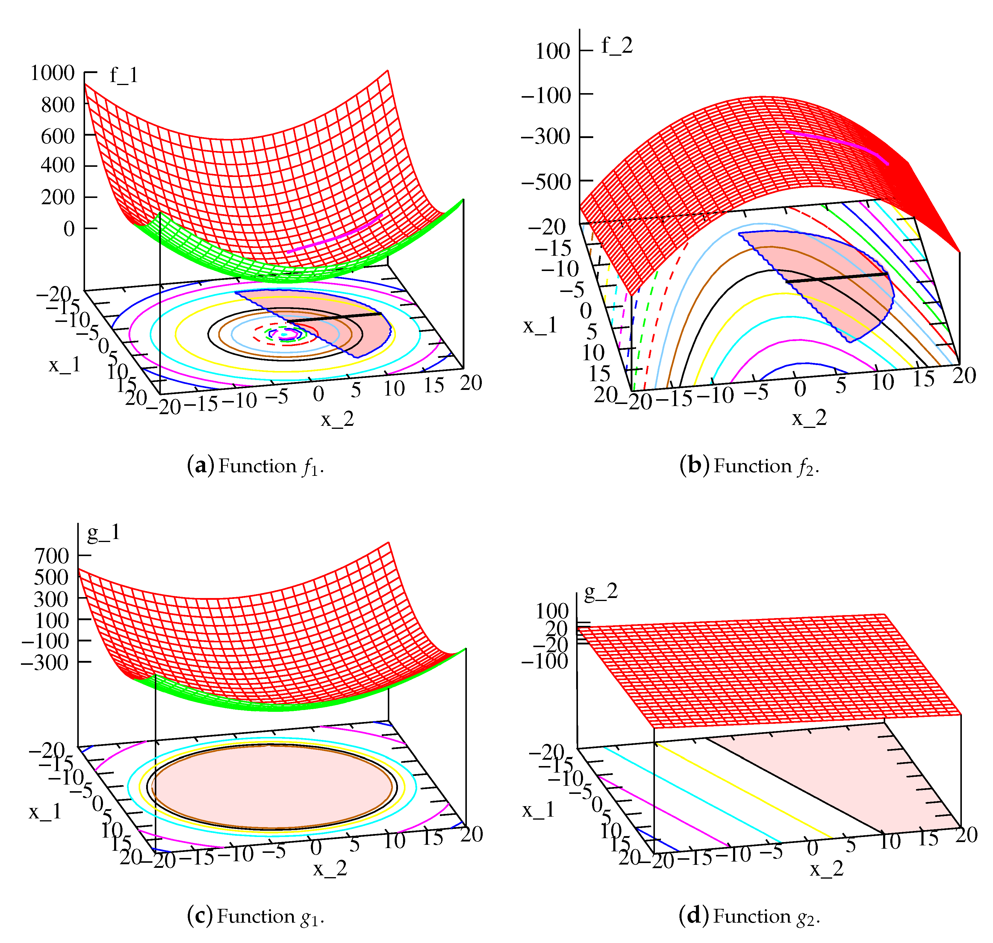
We explain each framework using a two-variable, two-objective SRN problem [
54,
55] as an example:
The PO solutions are known to be as follows:
and
. To apply a metamodeling approach, one simple idea is to metamodel all four functions. The functions and the respective PO solutions are marked on
and
plots shown in
Figure 2a,b, respectively. The feasible regions for
anf
are shown in
Figure 2c,d.
3.1. M1-1 and M1-2 Frameworks
Most existing multiobjective metamodeling approaches are found to fall in these two frameworks [
20]. In M1-1 and M1-2, a total of
metamodels (
M objectives and
J constraints) are constructed. The metamodeling algorithm for M1-1 and M1-2 starts with an archive of initial population (
of size
) created using the Latin hypercube sampling (LHS) method on the entire search space, or by using any other heuristics of the problem. Each objective function (
, for
) is first normalized to obtain a normalized function
using the minimum (
) and maximum (
) values of all high-fidelity evaluation of archive members, so that the minimum and maximum values of
is zero and one, respectively:
Then, metamodels are constructed for each of the
M normalized objective functions independently:
using a chosen metamodeling method. For all implementations here, we use the Kriging metamodeling method [
56] for all frameworks of this study.
Each constraint function (
, for
) is first normalized to obtain a normalized constraint function (
) using standard methods [
57], and then metamodeled separately to obtain an approximate function (
) using the same metamodeling method (Kriging method is adopted here) used for metamodeling objective functions.
In M1-1, all metamodeled normalized objectives are combined into a single
aggregated function and optimized with all separately metamodeled constraints to find a
single in-fill point using a single-objective evolutionary optimization algorithm (real-coded genetic algorithm (
RGA) [
54] is used here). In
generations of RGA (defining an epoch), the following achievement scalarization aggregation function (ASF
(
,
)) [
58] is optimized for every
vector:
where the vector
is one of the Das and Dennis’s [
59] point on the unit simplex on the
M-dimensional hyperspace (making
). Thus, for each of
H different
vectors, one optimization problem (O1-1) is formed with an equi-angled weight vector, and solved one at time to find a total of
H in-fill solutions using a real-parameter genetic algorithm (RGA).
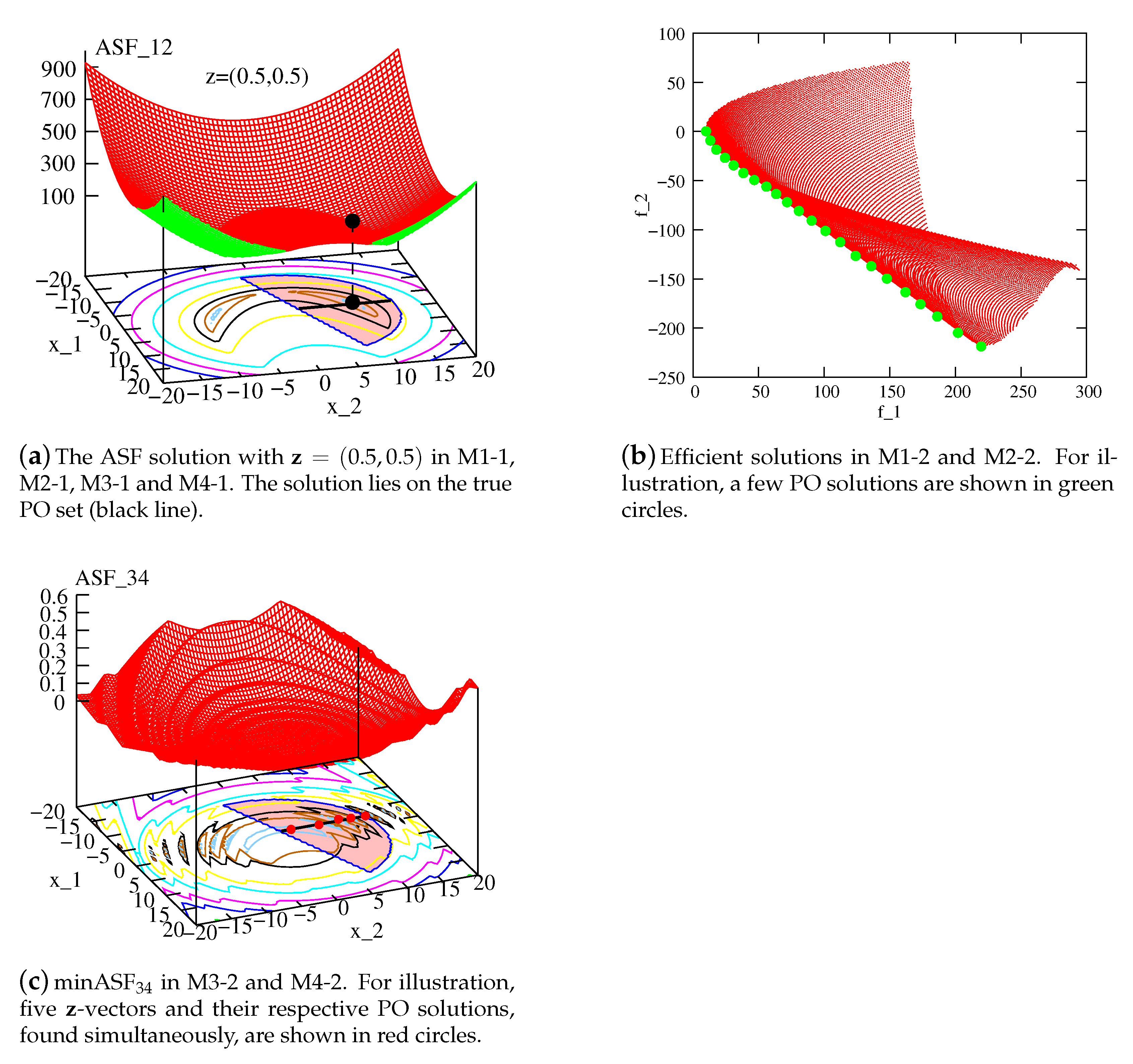
Figure 3a shows the infill solution for
for the SRN problem. Notice, the ASF
function constitutes a minimum point on the Pareto-optimal (PO) line (black line on the contour plot) for the specific
-vector. If the exact ASF
function can be constructed as a metamodeled function from a few high-fidelity evaluations, one epoch would be enough to find a representative PO set. However, since the metamodeled function is expected to have a difference from the original function, several epochs will be necessary to get close to the true PO set. For a different
-vector, the ASF
function will have a different optimal solution, but it will fall on the PO line. The ASF
model, constructed from metamodeled objective and constraint functions, will produce optimal solutions on the Pareto set for different
-vectors. Multiple applications of a RGA will discover a well-distributed set of multiple in-fill points one at a time.
The RGA procedure uses a
trust-region concept, which we describe in detail in
Section 4.3. The best solution for each
is sent for a high-fidelity evaluation. The solution is then included in the archive (
) of all high-fidelity solutions. After all
H solutions are included in the archive, one epoch of the M1-1 framework optimization problem is considered complete. In the next epoch, all high-fidelity solutions are used to normalize and metamodel all
objective functions and constraints, and the above process is repeated to obtain
. The process is continued until all prespecified maximum solution evaluations (SE
) is completed. Nondominated solutions of final archive
is declared as outcome of the whole multiobjective surrogate-assisted approach.
In M1-2, the following
M-objective optimization problem,
constructing
metamodels in each epoch, is solved to find
H in-fill solutions in a
single run with an EMO/EMaO procedure. We use NSGA-II procedure [
39] for two-objective problems, and NSGA-III [
60] for three or more objective problems here. All
H solutions are then evaluated using high-fidelity models and are included in the archive for another round of metamodel construction and optimization for the next epoch. The process is continued until SE
evaluations are done.
Figure 3b shows that when NSGA-II optimizes a well-approximated metamodel to the original problem, the obtained solutions will lie on the true PO front.
3.2. Frameworks M2-1 and M2-2
For M2-1 and M2-2, a single aggregated constraint violation function (ACV(
)) is first constructed using the normalized constraint functions (
,
) at high-fidelity solutions from the archive (
), as follows:
where the bracket operator
is
, if
; and zero, otherwise. It is clear from the above equation that for high-fidelity solutions, ACV(
) takes a negative value for feasible solutions and a positive value for an infeasible solution. In M2-1 and M2-2, the constraint violation function (ACV(
)) is then metamodeled to obtain
, instead of every constraint function (
) metamodeled in M1-1 and M1-2. This requires a total of
metamodel constructions (
M objectives and one constraint violation function) at each epoch. In M2-1, the following problem
is solved to find one in-fill point for each reference line originating from one of the chosen Das-Dennis reference points
. Similarly, M2-2 solves the following problem:
to find
H in-fill solutions simultaneously. The rest of the M2-1 and M2-2 procedures are identical to that in M1-1 and M1-2, respectively. RGA is used to solve each optimization problem in M2-1 to find one solution at a time, and NSGA-II or NSGA-III is used in M2-2 depending on number of objectives in the problem. Thus, M2-1 requires an archive to store each solution, whereas M2-2 does not require an archive.
3.3. M3-1 and M3-2 Frameworks
In these two methods, instead of metamodeling each normalized objective function
for
independently, we first aggregate them to form the following ASF
function for each high-fidelity solution
:
where
is defined as before. Note this formulation is different from ASF
in that the ASF formulation is made with the original normalized objective functions
here. Then, one ASF
function (for a specific
-vector) is metamodeled to obtain
, along with
J separate metamodels for
J constraints (
) to solve the following problem for M3-1:
For every
, a new in-fill point is found by solving the above problem using the same RGA, discussed for M1-1. Every in-fill point is stored in an archive to compare with M*-2 methods, which creates multiple solutions in one run, thereby not requiring an explicit archive. In M3-2, the following problem is solved:
in which the objective function of
is computed as the minimum
for all
-vectors at
.
Figure 3c shows the multimodal objective function minASF
for the SRN problem, clearly indicating multiple local optima on the PO front. Notice how the minASF
function has ridges and creates multiple optima on the PO set, one for each reference line. Due to the complexity involved in this function, it is clear that a large number of high-fidelity points will be necessary to make a suitable metamodel with a high accuracy. Besides the need of more points, there is another issue that needs a discussion. Both M3-1 and M3-2 requires
H,
and
J constraint functions to be metamodeled, thereby making a total of
metamodels in each epoch. Since each of multiple optima of the minASF
function will finally lead us to a set of PO solutions, we would need an efficient multimodal optimization algorithm, instead of a RGA, to solve the metamodeled minASF
function.
We use a
multimodal single-objective evolutionary algorithm to find
H multimodal in-fill points of minASF
simultaneously. We propose a multimodal RGA (or MM-RGA) which starts with a random population of size
N for this purpose. In each generation, the population (
) is modified to a new population (
) by using selection, recombination, and mutation operators. The selection operator emphasizes multiple diverse solutions as follows. First, a
fitness is assigned to each population member
by computing
for all
H,
-vectors and then assigning the smallest value as the fitness. Then, we apply the binary tournament selection to choose a parent using the following selection function:
where
is the maximum
value of all feasible population members of MM-RGA. The above selection function has the following effects. If two solutions are feasible,
is used to select the winner. If one is feasible and the other is infeasible, the former is chosen, and for two infeasible members, the one with smaller constraint violation
is chosen. After
N offspring population members are thus created, we merge the population to form a combined population of
members. The best solution to each
-vector is then copied to
. In the event of a duplicate, the second best solution for the
-vector is chosen. If
H is smaller than
N, then the process is repeated to select a second population member for as many
-vectors as possible. Thus, at the end of the MM-RGA procedure, exactly
H in-fill solutions are obtained.
3.4. Frameworks M4-1 and M4-2
In these two frameworks, constraints are first combined to a single constraint violation function ACV(
) as in M2-1 (Equation (
6)) and then ACV is metamodeled to obtain
. The following problem is then solved:
to find a single in-fill solution for every
. An archive is built with in-fill solutions. In M4-2, following problem is solved to find
H in-fill solutions simultaneously:
Both these frameworks require
H,
and one ACV function to be metamodeled, thereby making a total of
metamodels in each epoch. The same MM-RGA is used here, but the SF function is modified by replacing
term with
in Equation (
12). A similar outcome as in
Figure 3c occurs here, but the constraints are now handled using one metamodeled
function. M4-2 does not require an archive to be maintained, as
H solutions will be found in one MM-RGA application.
3.5. M5 Framework
The focus of M5 is to use a generative multiobjective optimization approach in which a single PO solution is found at a time for a
-vector by using a combined
selection function involving all objective and constraint functions together. The following
selection function is first created:
Here, the parameter
is the worst ASF
function value (described in Equation (
9)) of all feasible solutions from the archive. The selection function
(
,
) is then metamodeled to obtain
, which is then optimized by RGA (described for M1-1) to find one in-fill solution for each
-vector. The unconstrained optimization problem with only variable bounds is given below:
Thus,
H metamodels of
need to be constructed for M5 in each epoch.
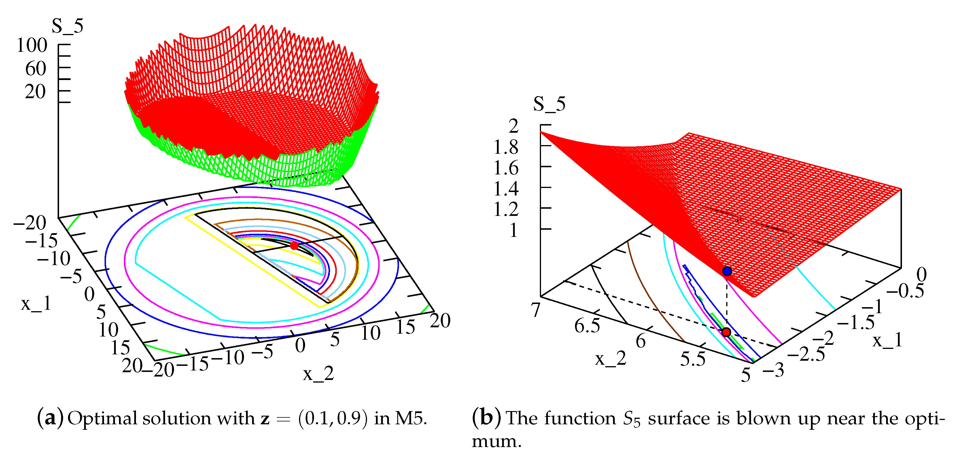
Figure 4a shows the
function with
for SRN problem. Although details are not apparent in this figure,
Figure 4b, plotted near the optimum, shows optimum more clearly. The entire surface plot is not shown for clarity, but it is interesting to see how a single function differentiates infeasible from feasible region and also makes the optimum of the function as one of the PO solutions.
Clearly, the complexity of the resulting function will demand a large number of archive points for an accurate identification of the PO solution or a large number of epochs to arrive at the PO solution. However, the concept of metamodeling a selection function, which is not one of the original objective or constraint function, to find an in-fill solution of the problem is intriguing and opens up a new avenue for surrogate-assisted multiobjective optimization studies.
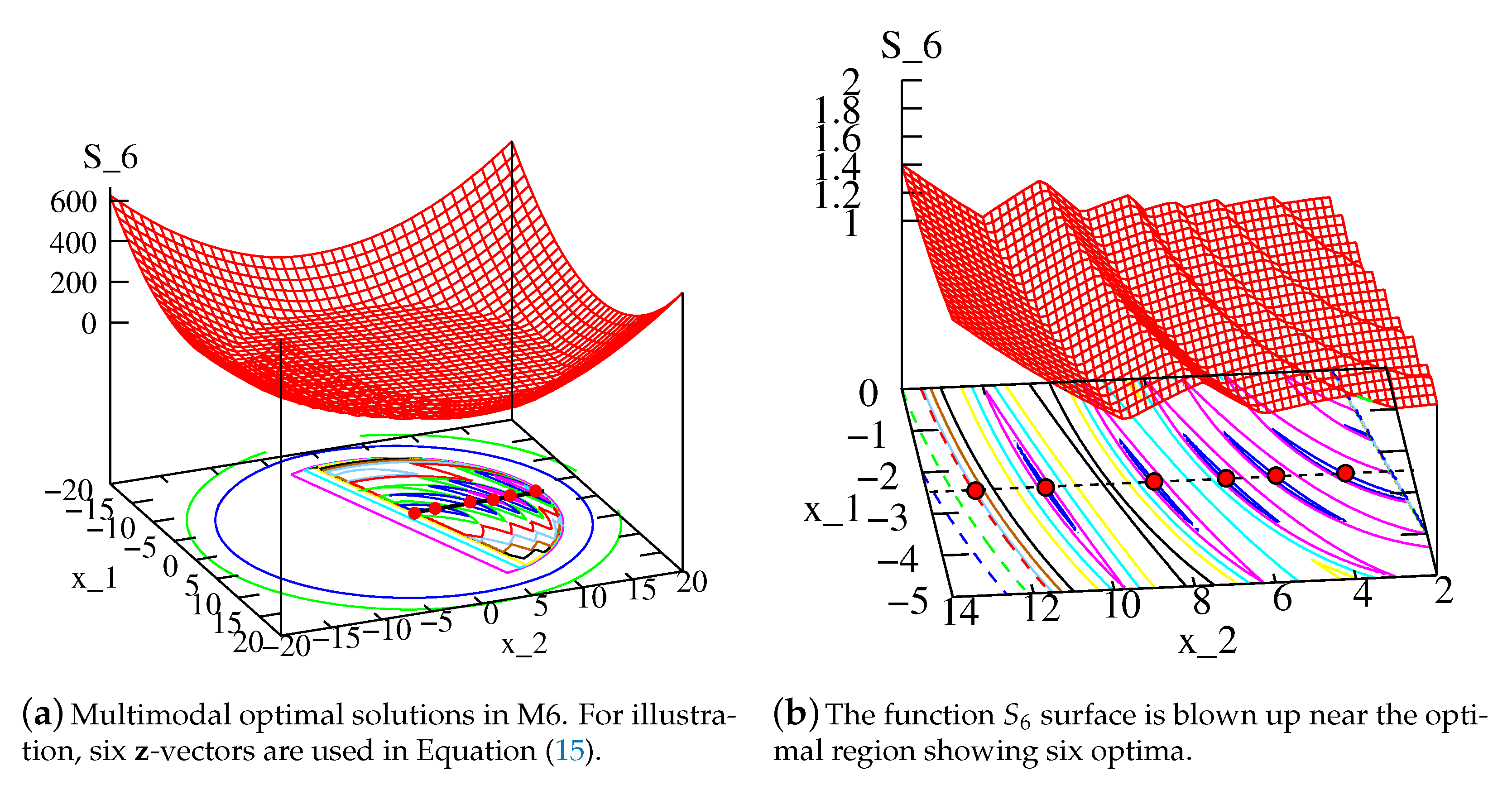
3.6. Framework M6
Finally, M6 framework takes the concept of M5 a bit further and constructs a single metamodel in each epoch by combining all
M objectives and
J constraints together. A multimodal selection function having each optimum corresponding to a distinct PO solution is formed for this purpose:
Then, the following selection function is constructed:
where ASF
is the maximum ASF
value of all feasible archive members. For each archive member
,
is first computed. CV(
) is same as ACV(
), except that for a feasible
, CV is set to zero. Then, the following multimodal unconstrained problem (with variable bounds) is constructed to find
H in-fill solutions simultaneously:
A single metamodel needs to be constructed in each epoch in M6 framework. Due to the complexity involved in the
-function, we employ a neural network
to metamodel this selection function. A niched RGA [
7] similar to that described in
Section 3.4 is used here to find
H in-fill solutions corresponding to each local optimum of the metamodeled
function. No explicit archive needs to be maintained to store
H solutions.
Figure 5a shows
function for SRN function on the entire search space. The detail inside the feasible region and near the optimal solutions shown in
Figure 5b makes it clear that this function creates six optima on the PO front, corresponding to six
-vectors. Although the function is multimodal, the detail structure from
Figure 5a to
Figure 5b can be modeled gradually with iterations of a carefully designed optimization algorithm.
3.7. Summary of 10 Frameworks
A summary of metamodeled functions and the optimization algorithms used to optimize them for all 10 frameworks is provided in
Table 1. The relative computational cost for each framework can be derived from this table. M3-1 and M3-2 require to construct the maximum number of metamodels (assuming the number of desired PO solutions
) among all the frameworks, and M6 requires the least, involving only one metamodel in each epoch.
The evolutionary algorithm used to solve each optimization problem is also provided in the table.
4. Adaptive Switching Based Metamodeling (ASM) Frameworks
Each metamodeling framework in our proposed taxonomy requires building metamodels for either each objective and constraint or their aggregations. Thus, it is expected that each framework may be most suitable for certain function landscapes that produce a smaller approximation error, but that framework may not be good in other landscapes. During an optimization process, an algorithm usually faces different kinds of landscape complexities from start to finish. Thus, no one framework is expected to perform best during each step of the optimization process. While each framework was applied to different multiobjective optimization problems in another study [
6,
20] from start to finish, different problems were found to be solved best by different frameworks. To determine the best performing framework for a problem, a simple-minded approach would be to apply each of the 10 frameworks to solve each problem independently using SE
high-fidelity evaluations, and then determine the specific framework which performs the best using an EMO metric, such as hypervolume [
61] or inverse generational distance (IGD) [
62]. This will be computationally expensive, requiring 10 times more than the prescribed SE
. If each framework is allocated only 1/10-th of SE
, they may be insufficient to find comparatively good solutions. A better approach would be to use an adaptive switching strategy that chooses the most suitable framework at each epoch.
As mentioned in the previous section, in each epoch, exactly
H new in-fill solutions are created irrespective of the metamodeling framework used, thereby consuming
H high-fidelity SEs. Clearly, the maximum number of epochs allowable is
with a minor adjustment on the SEs used in the final epoch. At the beginning of each epoch (say,
t-th epoch), we have an archive (
of
high-fidelity solutions. For the first epoch, these are all
Latin hypercube sampled (LHS) solutions, and in each subsequent epoch,
H new in-fill solutions are added to the archive. At the start of
t-th epoch, each of the 10 frameworks is used to construct its respective metamodels using all
archive members. Then, a 10-fold cross-validation method (described in
Section 4.2) is used with a suitable performance metric (described in
Section 4.1) to determine the most suitable framework for the next epoch. Thereafter, the best-performing framework is used to find a new set of
H in-fill solutions. They are evaluated using high-fidelity evaluations and all 10 frameworks are statistically compared to choose a new best-performing framework for the next epoch. This process is continued until SE
evaluations are made. A pseudocode of the proposed ASM approach is provided in Algorithm 1.
| Algorithm 1: Adaptive Swithing Framework |
![Mca 26 00005 i001]() |
4.1. Performance Metric for Framework Selection
To compare the performances among multiple surrogate models, mean squared error (MSE) has been widely used in literature [
30]. For optimization algorithms, the regression methods that use MSE are known to be susceptible to outliers. For multiple objectives, different objectives and constraints may have different scaling. Our pilot study shows that even with the normalization of the objectives and constraints, the MSE metric does not always correctly evaluate the metamodels. Here, we introduce a
selection error probability (SEP) metric which is more appropriate for an optimization task than MSE metric or even other measures, such as, the Kendal rank correlation coefficient [
63] metric. The usual metrics may be better for a regression task, but for an optimization task, the proposed SEP makes a more direct evaluation of pair-wise comparisons of solutions.
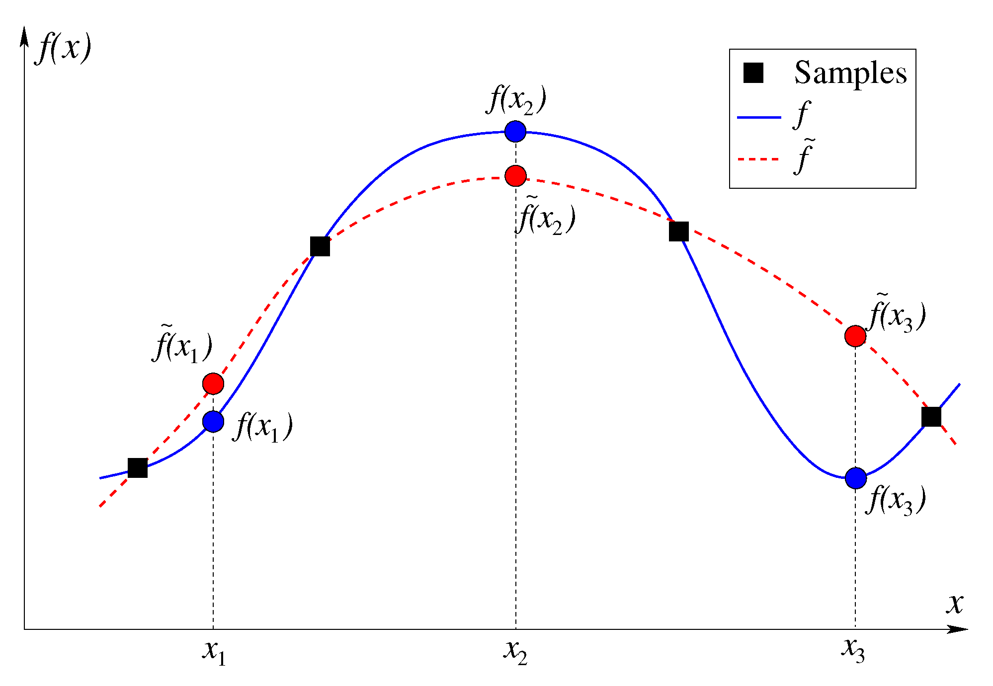
SEP is defined as the probability of making an error in correctly predicting the better of two solutions compared against each other using the constructed metamodels. Consider
Figure 6, which illustrates an minimization task and comparison of three different population members pair-wise. The true function values are shown in solid blue, while the predicted function values are shown in dashed blue. When points
and
are compared based on predicted function, the prediction is correct, since
and also
. However, when points
and
are compared against each other, the prediction is wrong. Out of the three pairwise comparisons, two predictions are correct and one is wrong, thereby making a selection error probability of 1/3 for this case. We argue that in an optimization procedure, it is the SEP which provides a better selection error than the actual function values, as the relative function values are important than the exact function values.
Mathematically, the SEP metric can be defined for
n points as follows. For each of
pairs of points (
p and
q), we evaluate the selection error function (
), which is one, if there is a mismatch between predicted winner and actual winner of
p and
q; zero, otherwise. Then, SEP is calculated as follows:
The definition of a “winner” can be easily extended to multiobjective and constrained multiobjective optimization by considering the domination [
64] and constraint-domination [
54] status of two points
p and
q.
4.2. Selecting a Framework for an Epoch
Frameworks having least SEP value are considered to be the best for performing the next epoch. We have performed 10-fold cross-validation in order to identify the best frameworks. After each epoch, H new in-fill points are evaluated using high-fidelity evaluations and added to the archive. In each fold of cross-validation, 90% solutions are used for constructing metamodels with respect to the competing frameworks. Then the corresponding frameworks are used to compare every pair (p and q) of the remaining 10% of archive points using the SEP metric. We apply constrained domination checks to identify the relationship between these two solutions. We then compare this relationship with the true relationship given by their high-fidelity values with the same constrained domination check. We calculate the selection error function () for each pair of test archive solutions. The above process is repeated 10 times by using different blocks of 90% points to obtain 10 different SEP values for each framework. This cross-validation procedure does not require any new solution evaluations, as the whole computations are performed based on the already-evaluated archive points and their predicted values from each framework. Thereafter, the best framework is identified based on the median SEP value of frameworks.
Finally, the Wilcoxon rank-sum test is performed between the best framework and all other frameworks. All frameworks within a statistical insignificance (having ) are identified to obtain the best-performing set . Then a randomly chosen framework () is selected from for the next epoch. Since each of these frameworks performs similarly in a sense of median performance, the choice of a random framework makes the ASM approach diverse with the probability of using different metamodeling landscapes in successive epochs. This procedure, in practice, prohibits the overall approach from getting stuck in similar metamodeling frameworks for long, even it is one of the best performing frameworks.
4.3. Trust-Region Based Real-Coded Genetic Algorithms
Before we present the results, we need to discuss one other algorithmic aspect, which is important. Since the metamodels are not error-free, predictions of solutions close to high-fidelity solutions are usually more accurate than predictions far from them. Therefore, we use a trust-region method [
65] in which predictions are restricted within a radius
from each high-fidelity solution in the variable space. Trust region method is used in nonevolutionary metamodeling studies [
35,
36]. Another parameter
is also introduced which defines the minimum distance with which any new solution should be located from an archive member to provide a diverse set of in-fill solutions. We simulate a feasible search region
around every high-fidelity solution:
. Using the concepts of trust-region method from the literature [
66], we reduce the two radii at every epoch by constant factors:
and
. A reduction of two radii helps in achieving more trust on closer to high-fidelity solutions with iterations. These factors are found to perform well on a number of trial-and-error studies prior to obtaining the results presented in the next section.
The optimization methods for metamodels are modified as follows. At generation t, parent population is applied by a standard binary constrained tournament selection on two competing population members using the metamodeled objectives, constraints, or selection criteria described before to choose the winner. Standard recombination and mutation operators (without any care for trust region concept) are used to create an offspring population, which is then combined with the parent population and then better half is chosen for the next generation as parent population using the trust region concept. We first count the number of solutions in the combined population within the two trust regions. If the number is smaller than or equal to N, then they are copied to and remaining slots are filled with solutions which are closest to the high-fidelity solutions in the variable space. On the other hand, if the number is larger than N, the same binary constrained tournament selection method is applied to pick N solutions from them and copied to .
6. Conclusions
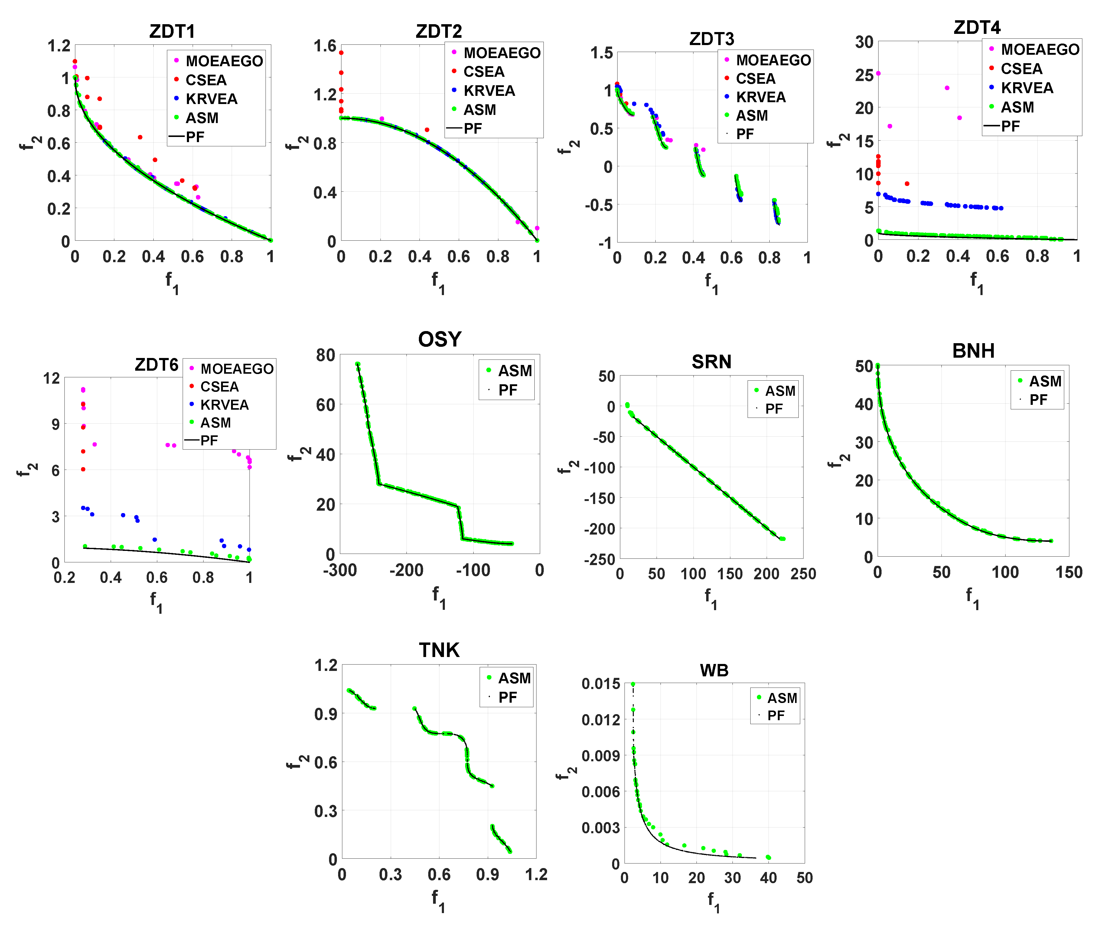
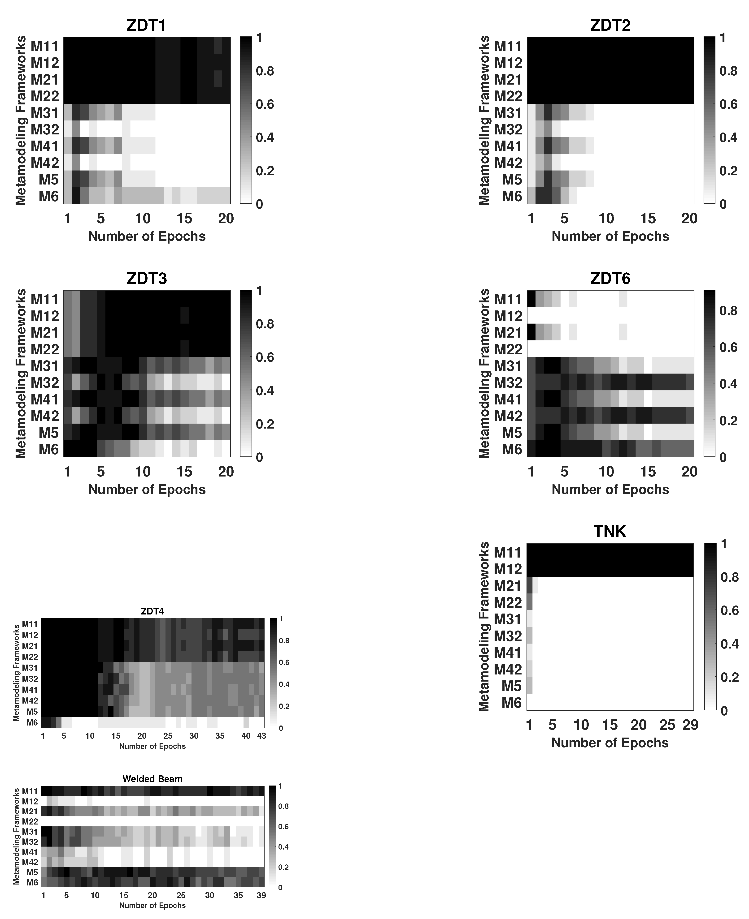
In this paper, we have provided a brief review of existing metamodeling methods for multiobjective optimization, since there has been a surge in such studies in the recent past. Since this calls for modeling multiple objectives and constraints in a progressive manner, a recently proposed taxonomy of 10 frameworks involving metamodeling of independent or aggregate functions of objectives and constraints have been argued to cover a wide variety such methods. Each framework has been presented in detail, comparing and contrasting them in terms of the number of metamodeling functions to be constructed, the number of internal optimization problems to be solved, and the type of optimization methods to be employed, etc. We have argued that each metamodeling framework may be ideal at different stages during an optimization run on an arbitrary problem, hence, an ensemble use of all 10 frameworks becomes a natural choice. To propose an efficient multiobjective metamodeling algorithm, we have proposed an adaptive switching based metamodeling (ASM) methodology which automatically chooses the most appropriate framework epoch-wise during the course of an optimization run. In order to choose the best framework in every epoch, we perform statistical tests based on a newly proposed acceptance criterion—selection error probability (SEP), which counts the correct pairwise relationships of objectives between two test solutions in a k-fold cross-validation test, instead of calculating the usual mean-squared error of metamodeled objective values from true values. We have observed that SEP is less sensitive to outliers and is much better suited for multiobjective constrained optimization. In each epoch, the ASM approach switches to an appropriate framework which then creates a prespecified number of in-fill points by using either an evolutionary single or multiobjective algorithm or by using a multimodal or a niche-based real-parameter genetic algorithm. On 18 test and engineering problems having two to five objectives and multiple constraints, the ASM approach has been found to perform much better compared to each framework alone and also to three other existing metamodeling multiobjective algorithms.
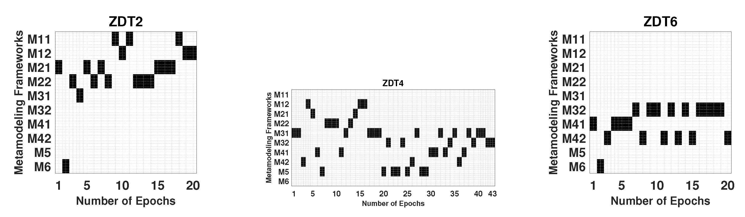
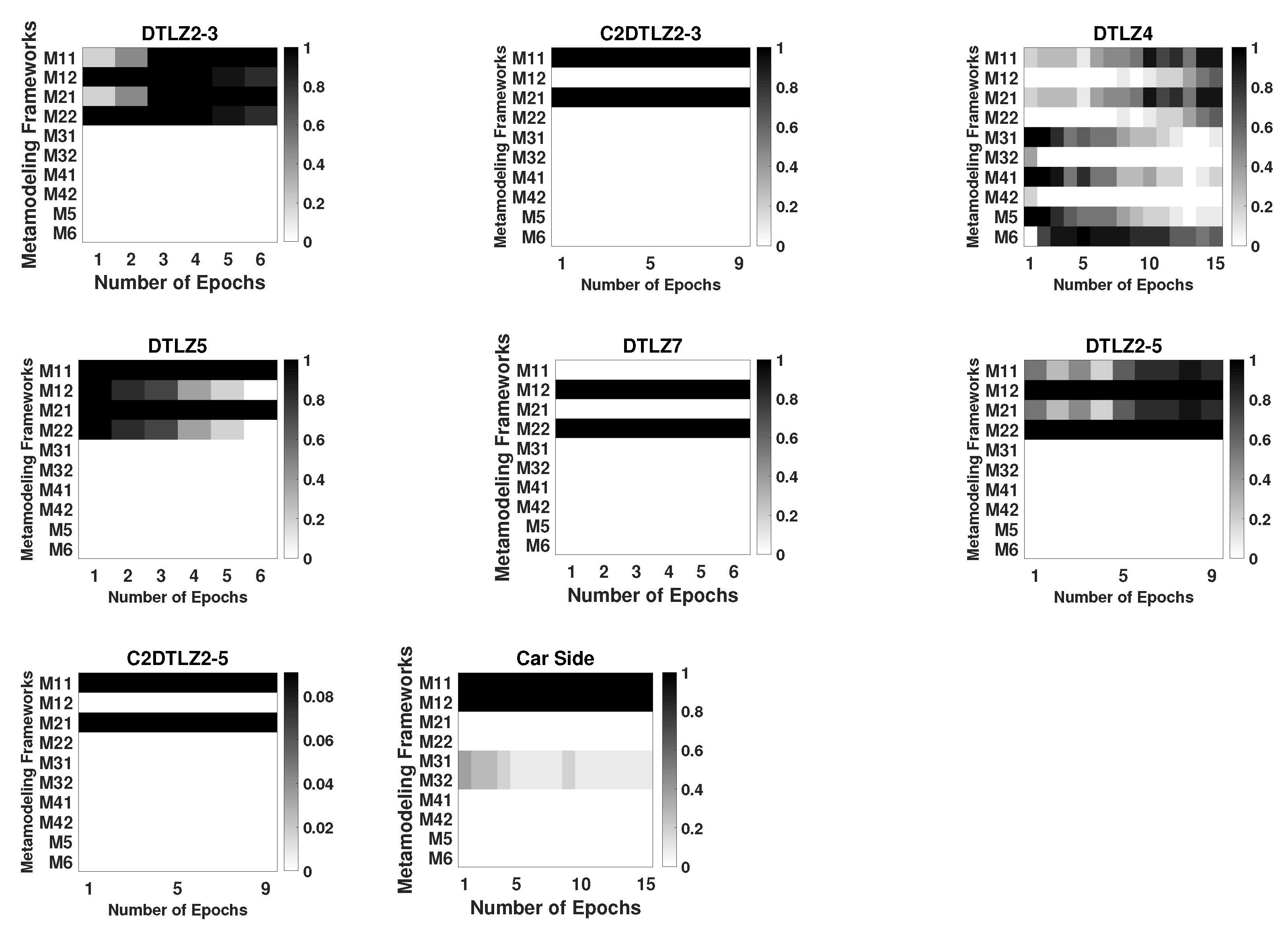
It has been observed that in most problems a switching between different M1 and M2 frameworks, in which objectives are independently metamodeled, has performed the best. Metamodeling of constraints in an aggregate manner or independently is not an important matter. However, for more complex problems, such as ZDT3, ZDT6, ZDT4, DTLZ4, and engineering design problems, all 10 frameworks, including M5 and M6, have been involved at different stages of optimization. Interestingly, certain problems have preferred to pick generative frameworks (Mi-1 and M5) only, while some others have preferred simultaneous frameworks (Mi-2 and M6). Clearly, further investigation is needed to decipher a detail problem-wise pattern of selecting frameworks, but this first study on statistics-based adaptive switching has clearly shown its advantage over each framework applied alone.
While in this paper, Kriging metamodeling method has been used for all frameworks, this study can be extended to choose the best metamodeling method from an ensemble of RBF, SVR, or other response surface methods to make the overall approach more computationally efficient. In many practical problems, some functions may be relatively less time-consuming, thereby creating a
heterogeneous metamodeling scenario [
16,
68,
69]. A simple extension of this study would be to formulate a heterogeneous
(for example, M1-1’s objective function for a two-objective problem involving a larger evaluation time for
can be chosen as
, in which the objective
has not been metamodeled at all). However, more involved algorithms can be tried for to handle such pragmatic scenarios. Another practical aspect comes from the fact that a cluster of objectives and constraints can come at the end of a single expensive evaluation procedure (such as, compliance objective and stress constraint comes after an expensive finite element analysis on a mechanical component design problem), whereas other functions come from a different time-scale evaluation procedure. The resulting definition of an epoch and the overall metamodeling approach need to be reconsidered to make the overall approach efficient. Other tricks, such as, the use of a low-fidelity evaluation scheme for expensive objective and constraints early on during the optimization process using a multifidelity scheme and the use of domain-informed heuristics to initialize population and repair offspring solutions must also be considered while developing efficient metamodeling approaches.


