HIV Dynamics with a Trilinear Antibody Growth Function and Saturated Infection Rate

Abstract

The objective of this paper is to study a new mathematical model describing the human immunodeficiency virus (HIV). The model incorporates the impacts of cytotoxic T lymphocyte (CTL) immunity and antibodies with trilinear growth functions. The boundedness and positivity of solutions for non-negative initial data are proved, which is consistent with biological studies. The local stability of the equilibrium is established. Finally, numerical simulations are presented to support our theoretical findings.

1. Introduction

The human immunodeficiency virus (HIV) is a virus that causes, at the end stage of infection, acquired immunodeficiency syndrome (AIDS). The human system then fails to perform its functions [1,2]. Several mathematical models of HIV dynamics have been developed in recent decades [3,4,5,6,7]. For example, reference [8] investigates a model representing the interaction between CD$4^{+}$ T cells, HIV contagions, and cytotoxic T lymphocyte (CTL) growth using two saturated rates defining viral infection and CTL proliferation. The authors demonstrate how the cellular immune response may be used to restrict the spread of HIV infections. Several recent studies have emphasized the importance of antibodies in reducing viral replication and improving patient quality of life [9,10,11,12]. The relevance of antibodies in infection control was recently examined by the authors of [13]. The essential novelty here is that antibody growth is dependent not only on the virus and antibody concentrations, but also on the uninfected cells’ concentration. It is very important, since the role of the immune response to HIV infection has been recently recognized by the medical literature to be of great value. Indeed, it is now well known that the CTL immune response increases depending on the infection. This increase also depends on the number of CTLs themselves. Moreover, the antibody immune response increases depending on the virus proliferation, and this growth also depends on the number of viruses. As the growth of the immune system cells depends on the number of healthy target cells (CD$4^{+}$ T cells), the development of immune responses is described using a trilinear term [14,15,16]. The objective of the HIV virus is to destroy CD$4^{+}$ T cells, often called messengers or the command centers of the immune system. Once the virus invades the body, these cells send a message to the immune system. CTLs and antibodies represent the immune system, which responds to this message and sets out to eliminate the infection by killing infected cells and free viruses. To include the antibodies in the model, their participation in controlling the infection is thus essential. Additionally, a comparison between simulations with HIV ordinary differential equation models and clinical data has been done in [17,18]. The following model has been presented:

$$\left\{\begin{array}{c}{\displaystyle \frac{dx}{dt}=\lambda -dx-\beta xv,}\hfill \\ {\displaystyle \frac{dy}{dt}=\beta xv-ay-pyz,}\hfill \\ {\displaystyle \frac{dv}{dt}=aNy-\mu v-qvw,}\hfill \\ {\displaystyle \frac{dz}{dt}=cxyz-hz,}\hfill \\ {\displaystyle \frac{dw}{dt}=gxvw-\sigma w}\hfill \end{array}\right.$$

In this model, $x\left(t\right),y\left(t\right),v\left(t\right),z\left(t\right)$, and $w\left(t\right)$, denote the concentrations of uninfected cells, infected cells, HIV virus, CTLs, and antibodies, respectively, at time t. The healthy $\mathrm{CD}{4}^{+}\mathrm{T}$ cells $\left(x\right)$ grow at a rate $\lambda$, die at a rate d, and become infected by the virus at a rate $\beta xv$. Infected cells $\left(y\right)$, die at a rate a and are killed by the CTLs response at a rate $p.$ Free virus $\left(v\right)$ is produced by the infected cells at a rate $aN$, die at a rate $\mu$, and decay in the presence of antibodies at a rate q, where N is the number of free viruses produced by each actively infected cell during its life time. CTLs $\left(z\right)$ expand in response to viral antigen derived from infected cells at a rate c and decay in the absence of antigenic stimulation at a rate h. Finally, antibodies $\left(w\right)$ develop in response to free viruses at a rate g and decay at a rate $\sigma$. It is worthwhile to note that all the model rates are assumed to be non-negative. We are interested in the same topic in this study, but we include the function of the CTL immune response and saturation rate in the model. The nonlinear system of five differential equations under investigation is as follows:

$$\left\{\begin{array}{c}{\displaystyle \frac{dx}{dt}=\lambda -dx-\frac{\beta xv}{1+\alpha v},}\hfill \\ {\displaystyle \frac{dy}{dt}=\frac{\beta xv}{1+\alpha v}-ay-pyz,}\hfill \\ {\displaystyle \frac{dv}{dt}=aNy-\mu v-qvw,}\hfill \\ {\displaystyle \frac{dz}{dt}=cxyz-hz,}\hfill \\ {\displaystyle \frac{dw}{dt}=gxvw-\sigma w}\hfill \end{array}\right.$$

(1)

where $\alpha$ is the saturated infection rate and the initial conditions are $x\left(0\right)=x_0$, $y\left(0\right)=y_0$, $v\left(0\right)=v_0$, $z\left(0\right)=z_0$, and $w\left(0\right)=w_0$.

The paper is organized as follows. Section 2 is devoted to the existence, positivity, and boundedness of solutions. The analysis of the model is carried out in Section 3. Then, in Section 4, the results are illustrated through numerical simulations. We finish in Section 5 with our conclusions.

2. Positivity and Boundedness of Solutions

It is generally known that any solutions reflecting cell densities should be non-negative and bounded. Therefore, it will be useful to establish the positivity and boundedness of solutions of the model (1). First of all, for biological results, the initial data $x_0$, $y_0$, $v_0$, $z_0$, and $w_0$ must be larger than or equal to 0. The main result of this section is given as follows:

Proposition 1.

For any non-negative initial conditions, the solutions to the problem (1) exist. In addition, this solution is non-negative and bounded for all $t\ge 0$.

Proof. 

First, we show that the non-negative ${\mathbb{R}}_{+}^5=\left\{(x,y,v,z,w)\in {\mathbb{R}}^5:\right.$$x\ge 0,y\ge 0,v\ge 0,z\ge 0$ and $w\ge 0\}$ is positively invariant. Additionally, for $(x\left(t\right),y\left(t\right),v\left(t\right),z\left(t\right),w\left(t\right))\in {\mathbb{R}}_{+}^5$, we have:

$$\begin{array}{cc}\hfill & {\dot{x}}_{x=0}=\lambda \ge 0,{\dot{y}}_{y=0}=\frac{\beta xv}{1+\alpha v}\ge 0,{\dot{v}}_{v=0}=aNy\ge 0,\hfill \\ \hfill & {\dot{z}}_{z=0}=0\ge 0,and{\dot{w}}_{w=0}=0\ge 0.\hfill \end{array}$$

Therefore, all solutions initiating in ${\mathbb{R}}_{+}^5$ are positive. Next, we prove that these solutions remain bounded. By adding the two first equations in (1), we have $\dot{B}=\lambda -dx-ay-pyz$; thus,

$$B\left(t\right)\le B\left(0\right)e^{-\delta t}+\frac{\lambda }{\delta }\left(1-e^{-\delta t}\right),$$

where $B\left(t\right)=x\left(t\right)+y\left(t\right)$ and $\delta =min(a;d).$ Since $1-e^{-\delta t}\le 1$ and $0\le e^{-\delta t}\le 1$, we deduce that $B\left(t\right)\le B\left(0\right)+\frac{\lambda }{\delta }$. Therefore, x and y are bounded. From the equation $\dot{v}=aNy-\mu v-qvw$, we deduce that

$$v\left(t\right)\le v\left(0\right)e^{-\mu t}+aN{\int }_0^{t}y\left(\xi \right)e^{(\xi -t)\mu }d\xi .$$

Then,

$$v\left(t\right)\le v\left(0\right)+\frac{aN}{\mu }{\parallel y\parallel }_{\infty }\left(1-e^{-\mu t}\right).$$

Since $1-e^{-\mu t}\le 1$, we have $v\left(t\right)\le v\left(0\right)+\frac{aN}{\mu }{\parallel y\parallel }_{\infty }$. Thus, v is bounded. Now, we prove the boundedness of z. From the fourth equation of (1), we have

$$\dot{z}\left(t\right)+hz\left(t\right)=cx\left(t\right)y\left(t\right)z\left(t\right).$$

Moreover, from the second equation of (1), it follows that

$$\dot{z}\left(t\right)+hz\left(t\right)=\frac{c}{p}x\left(t\right)(\beta x\left(t\right)v\left(t\right)-ay\left(t\right)-\dot{y}\left(t\right)).$$

By integrating over time, we have

$$z\left(t\right)=z\left(0\right)e^{-ht}+{\int }_0^t\frac{c}{p}x\left(s\right)(\beta x\left(s\right)v\left(s\right)-ay\left(s\right)-\dot{y}\left(s\right))e^{h(s-t)}ds.$$

From the boundedness of $x,y$, and v, and by using integration by parts, the boundedness of z follows. The two equations $\dot{v}\left(t\right)=aNy\left(t\right)-\mu v\left(t\right)-qv\left(t\right)w\left(t\right)$ and $\dot{w}\left(t\right)=gx\left(t\right)v\left(t\right)w\left(t\right)-\sigma w\left(t\right)$ imply

$$\dot{w}\left(t\right)+\sigma w\left(t\right)=gx\left(t\right)v\left(t\right)w\left(t\right)=\frac{g}{q}x\left(t\right)(aNy\left(t\right)-\dot{v}\left(t\right)-\mu v\left(t\right)).$$

Then,

$$w\left(t\right)=w\left(0\right)e^{-\sigma t}+{\int }_0^t\frac{g}{g}x\left(s\right)(aNy\left(s\right)-\mu v\left(s\right)-\dot{v}\left(s\right))e^{\sigma (s-t)}ds.$$

From the boundedness of x, y, and v, the boundedness of w follows. □

We established the well-posedness of the proposed model in this research, ensuring that all solutions exist and are bounded. This is consistent with the biological fact that these populations’ overall cell numbers are limited.

3. Analysis of the Model

In this section, we determine the steady states of the model (1).

3.1. Stability of the Disease-Free Equilibrium

The basic reproductive number of the system (1), is given by

$$R_0=\frac{\beta \lambda N}{d\mu }.$$

From a biological point of view, $R_0$ denotes the average number of secondary infections generated by one infected cell when all cells are uninfected. Moreover, the same system has the following disease-free equilibrium:

$$E_f=\left(\frac{\lambda }{d},0,0,0,0\right).$$

At any arbitrary point, the Jacobian matrix of the system (1) is given by

$$J=\left(\begin{array}{ccccc}-d-\frac{\beta v}{1+\alpha v}& 0\hfill & \frac{-\beta x}{{\left(1+\alpha v\right)}^2}& \hfill 0& 0\\ \frac{\beta v}{1+\alpha v}& -a-pz\hfill & \frac{\beta x}{{\left(1+\alpha v\right)}^2}& \hfill -py& 0\\ 0& aN\hfill & -\mu -qw& \hfill 0& -qv\\ cyz& cxz\hfill & 0& \hfill cxy-h& 0\\ gvw& 0\hfill & gxw& \hfill 0& gxv-\sigma \end{array}\right).$$

Proposition 2.

The disease-free equilibrium, $E_f$, is locally asymptotically stable for $R_0<1$.

Proof. 

At the disease-free equilibrium, $E_f$, the Jacobian matrix is given as follows:

$$J_{E_f}=\left(\begin{array}{ccccc}-d& 0\hfill & -\frac{\beta \lambda }{d}& 0& 0\\ 0& -a\hfill & \frac{\beta \lambda }{d}& 0& 0\\ 0& aN\hfill & -\mu & 0& 0\\ 0& 0\hfill & 0& -h& 0\\ 0& 0\hfill & 0& 0& -\sigma \end{array}\right).$$

The characteristic polynomial of $J_{E_f}$ is

$$P_{E_f}\left(X\right)=a_0{X}^5+a_1{X}^4+a_2{X}^3+a_3{X}^2+a_4{X}^1+a_5,$$

where

$$\begin{array}{cc}\hfill a_0=& 1,\hfill \\ \hfill a_1=& \sigma +h+\mu +a+d,\hfill \\ \hfill a_2=& \frac{\sigma da+a{d}^2+hda+\mu da+\sigma d^2+\sigma dh+\sigma d\mu +h{d}^2+\mu d^2+hd\mu -aN\beta \lambda }{d},\hfill \\ \hfill a_3=& \frac{a\sigma d^2+a\sigma dh+a\sigma d\mu +a{d}^{2}h+\mu d^{2}a+adh\mu +\sigma d^{2}h+\sigma d^2\mu +\sigma dh\mu +d^{2}h\mu }{d}\hfill \\ \hfill & -\frac{aN\sigma \beta \lambda +\alpha N\beta \lambda d+aNh\beta \lambda }{d},\hfill \\ \hfill a_4=& \frac{a\sigma d^{2}h+a\sigma d^2\mu +a\sigma dh\mu +a{d}^{2}h\mu +\sigma d^{2}h\mu -aN\sigma d\beta \lambda -aN\sigma h\beta \lambda -aNdh\beta \lambda }{d},\hfill \\ \hfill a_5=& \sigma h\mu da(1-R_0).\hfill \end{array}$$

By the Routh–Hurwitz theorem [19] applied to the fifth-order polynomial, the eigenvalues of the Jacobian matrix have negative real parts, since we have $a_1>0$, $a_1{a}_2>a_3,a_1{a}_2{a}_3>a_1^2{a}_4$, and $a_1{a}_2{a}_3{a}_4>a_1{a}_2^2{a}_5+a_1^2{a}_4^2$. Consequently, we obtain the asymptotic local stability of the disease-free equilibrium $E_f$. □

3.2. Infection Steady States

We now show the existence and stability of the infected steady states. All these steady states exist when the basic reproduction number exceeds unity, and disease invasion is always possible. In fact, it is easily verified that the system (1) has four of them:

$$\begin{array}{c}{E}_1=\left(x_1,y_1,v_1,0,0\right),\\ x_1=\frac{\mu \left(d{R}_0+\lambda \right)}{N\lambda \left(\alpha d+\beta \right)},y_1=\frac{d\mu \left(R_0-1\right)}{aN\left(\alpha d+\beta \right)},v_1=\frac{d\mu \left(R_0-1\right)}{\mu \left(\alpha d+\beta \right)}.\\ \\ E_2=\left(x_2,y_2,v_2,z_2,0\right),\\ x_2=\frac{\lambda \left(\alpha v_2+1\right)}{\alpha d{v}_2+\beta v_2+d},y_2=\frac{\mu }{aN}{v}_2,\\ z_2=\frac{a\left(-\alpha d\mu v_2+N\beta \lambda -d\mu -\beta \mu v_2\right)}{p\mu \left(\alpha d{v}_2+\beta v_2+d\right)},\\ v_2=\frac{\sqrt{a^2{h}^2{(\alpha d+\beta )}^2{N}^2+2achu\lambda (\alpha d-\beta )N+c^2{\lambda }^2{u}^2}+(\alpha d+\beta )haN-c\lambda u}{2\alpha c\lambda u}.\end{array}$$

$$\begin{array}{c}{E}_3=\left(x_3,y_3,v_3,0,w_3\right),\\ x_3=\frac{\lambda \left(\alpha v_3+1\right)}{\alpha d{v}_3+\beta v_3+d},y_3=\frac{\beta \lambda }{a\left(\alpha d{v}_3+\beta v_3+d\right)}{v}_3,\\ w_3=\frac{-\alpha d\mu v_3+N\beta \lambda -\beta \mu v_3-d\mu }{q\left(\alpha d{v}_3+\beta v_3+d\right)},\\ v_3=\frac{(\alpha d+\beta )\sigma -g\lambda +\sqrt{{(\alpha d+\beta )}^2{\sigma }^2+2g\lambda (\alpha d-\beta )\sigma +g^2{\lambda }^2}}{2g\lambda \alpha }.\\ E_4=\left(x_4,y_4,v_4,z_4,w_4\right)\\ x_4=\frac{\lambda \left(\alpha v_4+1\right)}{\alpha d{v}_4+\beta v_4+d},y_4=\frac{gh}{\sigma c}{v}_4,w_4=\frac{Nagh-\sigma c\mu }{\sigma cq},\\ z_4=-\frac{a\alpha dgh{v}_4+a\beta gh{v}_4+adgh-\alpha \beta c\lambda }{gph\left(\alpha d{v}_4+\beta v_4+d\right)},\\ v_4=\frac{(\alpha d+\beta )\sigma -g\lambda +\sqrt{{(\alpha d+\beta )}^2{\sigma }^2+2g\lambda (\alpha d-\beta )\sigma +g^2{\lambda }^2}}{2g\lambda \alpha }.\end{array}$$

In this case, the endemic equilibrium point $E_1$ represents the equilibrium case in the absence of an adaptive immune response. The endemic equilibrium points $E_2$ and $E_3$ define the equilibrium case in the presence of only one kind each of adaptive immune response, antibody response, and CTL response, respectively. The last endemic equilibrium point, $E_4$, is for chronic HIV infection with the presence of both kinds of adaptive immune response, CTLs and antibody. To study the stability of the points $E_1,E_2,E_3$, and $E_4$, we need the following reproduction numbers:

$$R_1=\frac{u(\alpha d+\beta )}{(N\alpha \lambda +u)\beta },$$

$$R_2=\frac{N\left(N\alpha \beta g{\lambda }^2-{\alpha }^2{d}^2\sigma -\alpha dg\lambda u-2\alpha \beta d\sigma +\beta g\lambda u-{\beta }^2\sigma \right)}{u^{2}dg},$$

$$R_3=\frac{g}{2c\sigma \mu }\frac{{\left(aNh\left(\alpha d+\beta \right)+\sqrt{a{N}^2{h}^2{\left(\alpha d+\beta \right)}^2+2aNch\lambda \mu \left(\alpha d-\beta \right)+c^2{\lambda }^2{\mu }^2}\right)}^2-c^2{\lambda }^2{\mu }^2}{\left(\left(\alpha d+\beta \right)\left(aNh\left(\alpha d+\beta \right)-c\lambda \mu +\sqrt{a{N}^2{h}^2{\left(\alpha d+\beta \right)}^2+2aNch\lambda \mu \left(\alpha d-\beta \right)+c^2{\lambda }^2{\mu }^2}\right)+2d\alpha c\lambda \mu \right)},$$

and

$$R_4=\frac{c\beta {\lambda }^2\alpha }{ah}\frac{\left(\sigma \left(\alpha d+\beta \right)+\sqrt{{\sigma }^2{\left(\alpha d+\beta \right)}^2+2\sigma g\left(\alpha d-\beta \right)+g^2{\lambda }^2}+g\lambda \right)}{\left(\left(\alpha d+\beta \right)\left(\sigma \left(\alpha d+\beta \right)+\sqrt{{\sigma }^2{\left(\alpha d+\beta \right)}^2+2\sigma g\left(\alpha d-\beta \right)+g^2{\lambda }^2}\right)+g\lambda \left(\alpha d-\beta \right)\right)}.$$

For the first point, $E_1$, we have the following result.

Proposition 3.

If $R_0>1$, then $E_1$ is locally asymptotically stable for $R_2<1$ and $R_1<1$.

Proof. 

If $R_0>1$, then the Jacobian matrix at $E_1$ is given by

$$J_{E_1}=\left(\begin{array}{ccccc}-d-\beta \frac{v_1}{1+\alpha v_1}& 0\hfill & -\beta \frac{x_1}{{\left(1+\alpha v_1\right)}^2}& 0& 0\\ \beta \frac{v_1}{1+\alpha v_1}& -a\hfill & \beta \frac{x_1}{{\left(1+\alpha v_1\right)}^2}& -p{y}_1& 0\\ 0& aN\hfill & -\mu & 0& -q{v}_1\\ 0& 0\hfill & 0& c{x}_1{y}_1-h& 0\\ 0& 0\hfill & 0& 0& g{x}_1{v}_1-\alpha \end{array}\right).$$

Its characteristic equation is

$$\left(c{x}_1{y}_1-h-X\right)\left(g{x}_1{v}_1-\sigma -X\right)\left(b_0{X}^3+b_1{X}^2+b_{2}X+b_3\right)=0$$

where

$$\begin{array}{cc}\hfill b_0& =1,\hfill \\ \hfill b_1& =a+d+\mu +\frac{\beta d\left(R_0-1\right)}{\beta +\alpha d{R}_0},\hfill \\ \hfill b_2& =a\mu +d\left(a+\mu \right)+\frac{1}{\beta +\alpha d{R}_0}\left(\beta d\left(a+\mu \right)\left(R_0-1\right)-a\mu d\left(\beta +\alpha d\right)\right),\hfill \\ \hfill b_3& =a\mu d+\frac{\beta \left(a\mu d\left(R_0-1\right)-a\lambda Nd\left(\beta +\alpha d\right)\left(R_0-1-\frac{1}{R_0}\left(1-\frac{\lambda \alpha }{d}-\frac{\mu }{dN}\right)\right)\right)}{\beta +\alpha d{R}_0}.\hfill \end{array}$$

Direct calculations lead to

$$g{x}_1{v}_1-\sigma =A_1\left(R_2-1\right)\mathrm{and}c{x}_1{y}_1-h=B_1\left(R_1-1\right)$$

with

$$A_1=\frac{dg\mu }{N{\left(\alpha d+\beta \right)}^2}\mathrm{and}{B}_1=\frac{dc{\mu }^2}{a{N}^2{\left(\alpha d+\beta \right)}^2}$$

The sign of the eigenvalue $A_1\left(R_2-1\right)$ is negative if $R_2<1$, zero if $R_2=1$, and positive if $R_2>1$. The sign of the eigenvalue $B_1\left(R_1-1\right)$ is negative if $R_1<1$, zero if $R_1=1$, and positive if $R_1>1$. On the other hand, we have $b_1>0$ and $b_1-b_2{b}_3>0$ (as $R_0>1$). From the Routh–Hurwitz theorem [19], the other eigenvalues of the above matrix have negative real parts. □

For the second endemic-equilibrium point $E_2$, we have the following result.

Proposition 4.

If $R_1>1$ and $R_3\le 1$, then $E_2$ is locally asymptotically stable.

Proof. 

We assume that $R_1>1$. The Jacobian matrix of $E_2$ is given as follows:

$$J_{E_2}=\left(\begin{array}{ccccc}-d-\frac{\beta v_2}{1+\alpha v_2}& 0\hfill & -\frac{\beta x_2}{{\left(1+\alpha v_2\right)}^2}& \hfill 0& 0\\ \frac{\beta v_2}{1+\alpha v_2}& -a-p{z}_2\hfill & \frac{\beta x_2}{{\left(1+\alpha v_2\right)}^2}& \hfill -p{y}_2& 0\\ 0& aN\hfill & -\mu & \hfill 0& -q{v}_2\\ c{y}_2{z}_2& c{x}_2{z}_2\hfill & 0& \hfill c{x}_2{y}_2-h& 0\\ 0& 0\hfill & 0& \hfill 0& g{x}_2{v}_2-\sigma \end{array}\right)$$

The characteristic equation of the system (1) at the point $E_2$ is given by

$$\left(g{x}_2{v}_2-\sigma -X\right)\left(c_0{X}^4+c_1{X}^3+c_2{X}^2+c_{3}X+c_4\right)=0$$

where

$$\begin{array}{cc}\hfill c_0& =1,\hfill \\ \hfill c_1& =d+a+\mu +\frac{\beta v_2}{1+\alpha v_2}+p{z}_2,\hfill \\ \hfill c_2& =\left(d+\frac{\beta v_2}{1+\alpha v_2}\right)\left(a+\mu \right)+a\mu +p{z}_2\left(d+\mu +h+\frac{\beta v_2}{1+\alpha v_2}\right)-\frac{aN\beta x_2}{{\left(1+\alpha v_2\right)}^2},\hfill \\ \hfill c_3& =a\mu \left(d+\frac{\beta v_2}{1+\alpha v_2}\right)+p{z}_2\left(\mu d+hd+\mu h+\mu \frac{\beta v_2}{1+\alpha v_2}+h\frac{\beta v_2}{1+\alpha v_2}\right)-\frac{aN\beta d{x}_2}{{\left(1+\alpha v_2\right)}^2},\hfill \\ \hfill c_4& =p{z}_2\left(\mu hd+\mu h\frac{\beta v_2}{1+\alpha v_2}-aN\beta h{y}_2\right).\hfill \end{array}$$

Simple calculations lead to

$$g{x}_2{v}_2-\sigma =\sigma \left(R_3-1\right).$$

Then, $g{x}_2{v}_2-\sigma =\sigma \left(R_3-1\right)$ is an eigenvalue of $J_{E_2}$. The sign of this eigenvalue is negative if $R_3<1$, null when $R_3=1$, and positive if $R_3>1$. On the other hand, from the Routh–Hurwitz theorem [19], the other eigenvalues of the above matrix have negative real parts when $R_1>1$. □

For the third endemic-equilibrium point $E_3$, the following result holds.

Proposition 5.

If $R_2>1$, then $E_3$ is locally asymptotically stable for $R_4<1$.

Proof. 

We assume that $R_2>1$. The Jacobian matrix of the system at point $E_3$ is given by

$$J_{E_3}=\left(\begin{array}{ccccc}-d-\frac{\beta v_3}{1+\alpha v_3}& 0\hfill & -\frac{\beta x_3}{{\left(1+\alpha v_3\right)}^2}& \hfill 0& 0\\ \beta \frac{\beta v_3}{1+\alpha v_3}& -a\hfill & \frac{\beta x_3}{{\left(1+\alpha v_3\right)}^2}& \hfill -p{y}_3& 0\\ 0& aN\hfill & -\mu -q{w}_3& \hfill 0& -q{v}_3\\ 0& 0\hfill & 0& \hfill c{x}_3{y}_3-h& 0\\ g{v}_3{w}_3& 0\hfill & g{x}_3{w}_3& \hfill 0& g{x}_3{v}_3-\sigma \end{array}\right).$$

The characteristic equation associated with $J_{E_3}$ is given by

$$\left(c{x}_3{y}_3-h-X\right)\left(d_0{X}^4+d_1{X}^3+d_2{X}^2+d_{3}X+d_4\right)=0$$

where

$$\begin{array}{cc}\hfill d_0& =1,\hfill \\ \hfill d_1& =a+d+\mu +\frac{\beta v_3}{1+\alpha v_3}+q{w}_3,\hfill \\ \hfill d_2& =\left(d+\frac{\beta v_3}{1+\alpha v_3}\right)(a+\mu )+a\mu +\left(d+a+\sigma +\frac{\beta v_3}{1+\alpha v_3}\right)q{w}_3-aN\frac{\beta x_3}{{\left(1+\alpha v_3\right)}^2},\hfill \\ \hfill d_3& =a\mu \left(d+\frac{\beta v_3}{1+\alpha v_3}\right)+\left(ad+\sigma d+a\sigma +a\frac{\beta v_3}{1+\alpha v_3}\right)q{w}_3-aNd\frac{\beta x_3}{{\left(1+\alpha v_3\right)}^2},\hfill \\ \hfill d_4& =ad\sigma q{w}_3.\hfill \end{array}$$

Here, $c{x}_3{y}_3-h$ is an eigenvalue of $J_{E_3}$. By assuming $c{x}_3{y}_3-h=h\left(R_4-1\right)$, we deduce that the sign of this eigenvalue is negative when $R_4<1$, zero when $R_4=1$, and positive for $R_4>1$. On the other hand, from the Routh–Hurwitz theorem [19], the other eigenvalues of the above matrix have negative real parts when $R^W>1$. Consequently, $E_3$ is locally asymptotically stable when $R_2>1$ and $R_4<1$. □

For the last endemic-equilibrium point $E_4$, we prove the following result.

Proposition 6.

If $R_3>1$ and $R_4>1$, then $E_4$ is locally asymptotically stable.

Proof. 

The Jacobian matrix of the system at the point $E_4$ is given by

$$J_{E_4}=\left(\begin{array}{ccccc}-d-\frac{\beta v_4}{1+\alpha v_4}& 0\hfill & -\frac{\beta x_4}{{\left(1+\alpha v_4\right)}^2}& 0& 0\\ \frac{\beta v_4}{1+\alpha v_4}& -a-p{z}_4\hfill & \frac{\beta x_4}{{\left(1+\alpha v_4\right)}^2}& -p{y}_4& 0\\ 0& aN\hfill & -\mu -q{w}_4& 0& -q{v}_4\\ c{y}_4{z}_4& c{x}_4{z}_4\hfill & 0& c{x}_4{y}_4-h& 0\\ g{v}_4{w}_4& 0\hfill & g{x}_4{w}_4& 0& g{x}_4{v}_4-\sigma \end{array}\right)$$

The characteristic equation associated with $J_{E_4}$ is given by

$$f_0{X}^5+f_1{X}^4+f_2{X}^3+f_3{X}^2+f_{4}X+f_5=0$$

where

$$\begin{array}{cc}\hfill f_0=& 1,\hfill \\ \hfill f_1=& a+d+\mu +\frac{\beta v_4}{1+\alpha v_4}+p{z}_4+q{w}_4,\hfill \\ \hfill f_2=& \left(d+\frac{\beta v_4}{1+\alpha v_4}\right)(a+\mu )+a\mu +p{z}_4\left(d+h+\mu +\frac{\beta v_4}{1+\alpha v_4}+q{w}_4\right)\hfill \\ & +q{w}_4\left(d+a+\sigma +\frac{\beta v_4}{1+\alpha v_4}\right)-aN\frac{\beta x_4}{{\left(1+\alpha v_4\right)}^2},\hfill \\ \hfill f_3=& a\mu \left(d+\frac{\beta v_4}{1+\alpha v_4}\right)+p{z}_4\left(d\mu +dh+\mu h+\mu \frac{\beta v_4}{1+\alpha v_4}+h\frac{\beta v_4}{1+\alpha v_4}\right)\hfill \\ & +q{w}_4\left(ad+\sigma d+a\sigma +a\frac{\beta v_4}{1+\alpha v_4}\right)+pq{z}_4{w}_4\left(d+\sigma +h+\frac{\beta v_4}{1+\alpha v_4}\right)\hfill \\ & -aNd\frac{\beta x_4}{{\left(1+\alpha v_4\right)}^2},\hfill \\ \hfill f_4=& adq{w}_4+p{z}_4\left(dh\mu +\mu h\frac{\beta v_4}{1+\alpha v_4}-aN\beta h{y}_4\right)+pq{z}_4{w}_4\left(d\sigma +\sigma \frac{\beta v_4}{1+\alpha v_4}+h\sigma \right),\hfill \\ \hfill f_5=& \sigma hd\left(pq{z}_4{w}_4+aN\frac{\beta v_4}{1+\alpha v_4}\left(1-\frac{\beta x_4}{1+\alpha v_4}\right)\right).\hfill \end{array}$$

From the Routh–Hurwitz theorem applied to the five-order polynomial, the eigenvalues of the Jacobian matrix have negative real parts, since we have $f_1>0$, $f_1{f}_2>f_3,f_1{f}_2{f}_3>f_1^2{f}_4$, and $f_1{f}_2{f}_3{f}_4>f_1{f}_2^2{f}_5+f_1^2{f}_4^2$. Consequently, we can obtain the asymptotic local stability of the endemic point $E_4$. □

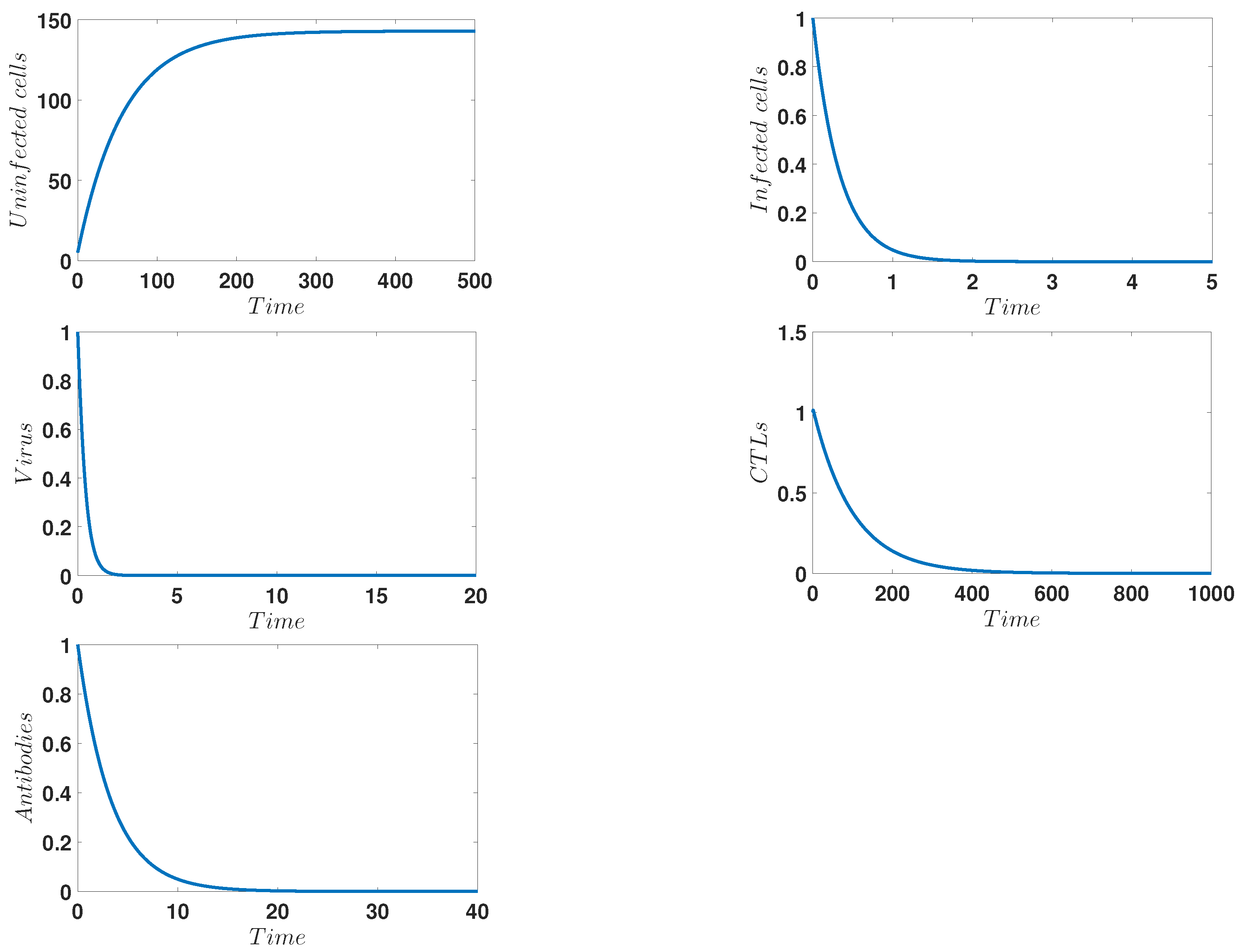
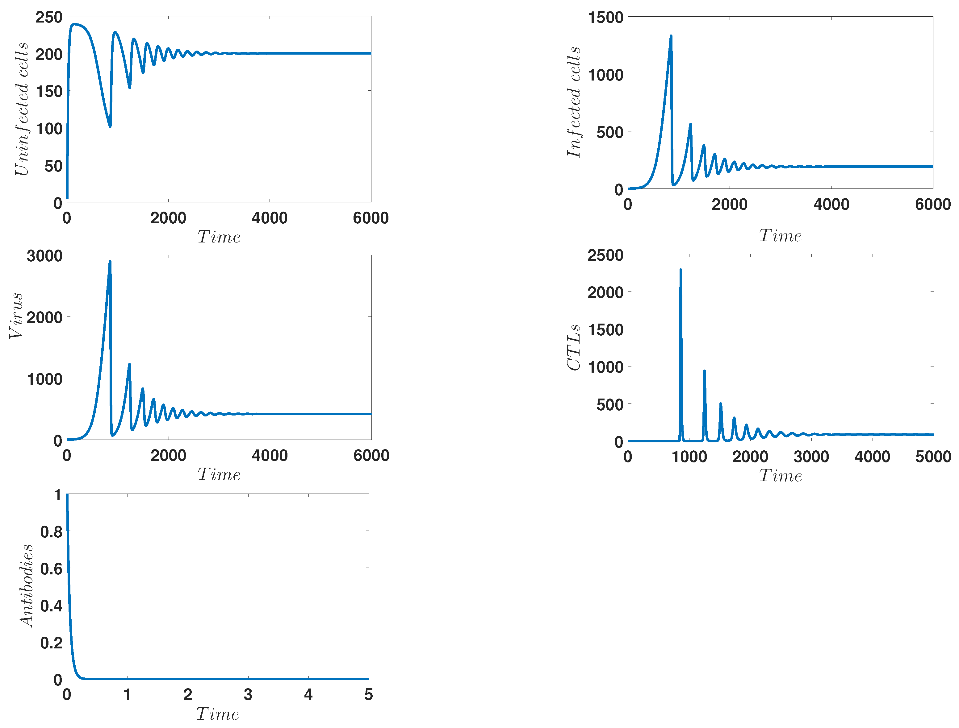
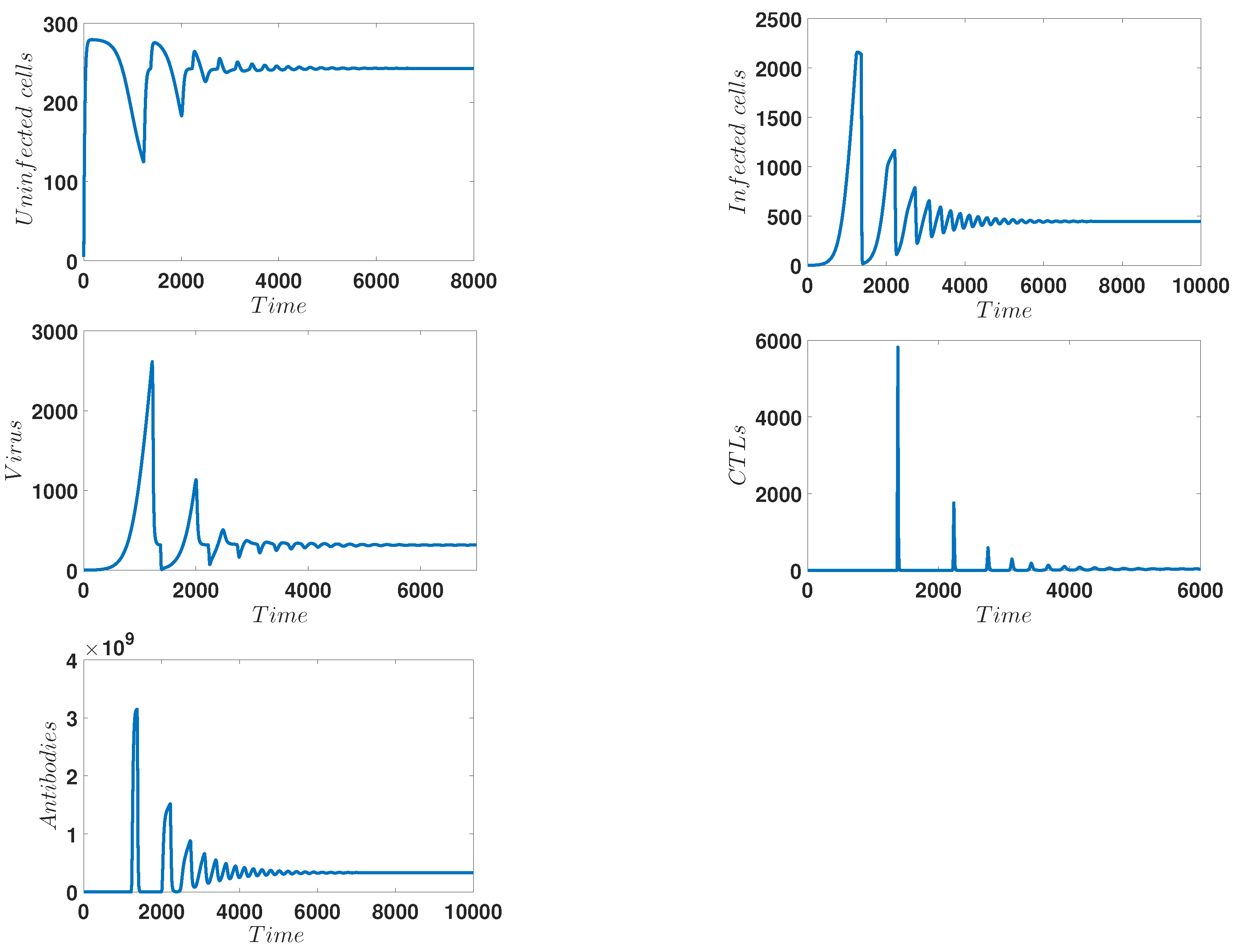
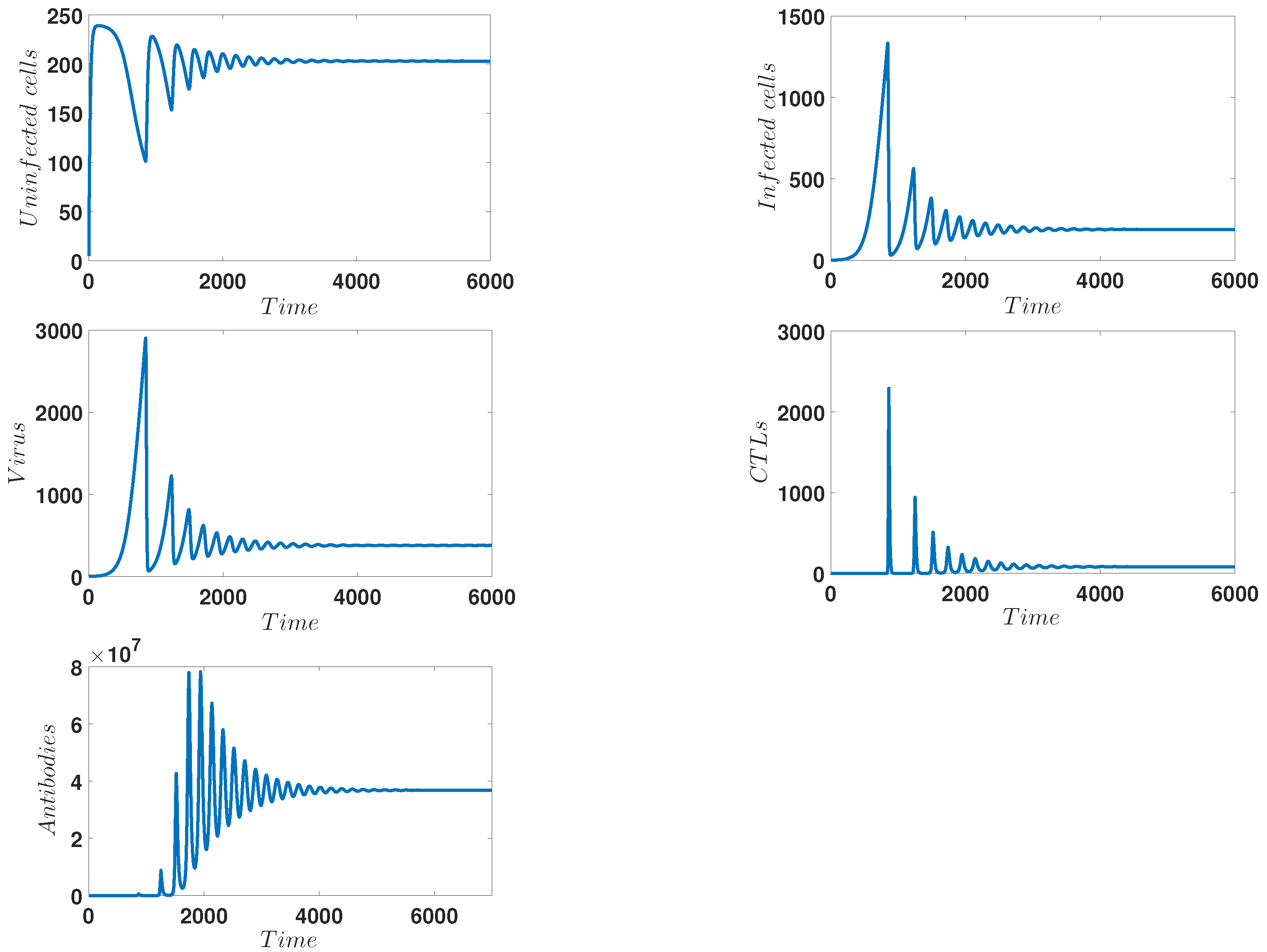
4. Numerical Simulations

The numerical simulations were performed using in-house code run in MATLAB software. To solve numerically the five differential equations of the system (1), numerical simulations have been carried out. The simulation parameters were derived from [13,19,20,21]. Our first numerical simulations were focused on demonstrating the importance of antibodies to reducing infection severity. Other numerical simulations was used to verify our theoretical findings. We also take into account the initial conditions given as follows: $x_0=5,y_0=1,v_0=1,z_0=1$, and $w_0=1$.

Figure 1 shows the development of the infection in the free equilibrium case: $d=0.007$, $\beta =0.00025$, $a=0.2$, $p=1$, $\mu =2.06$, $c=0.0051$, $h=0.004$, $\lambda =1$, $N=6.25$, $g=0.00013$, $q=0.12$, $\alpha ={10}^{-4}$, and $\sigma =0.12$. Within these chosen parameters, we have the basic reproduction number being less than unity $R_0=0.1084<1$, and we can observe the convergence of the curves corresponding to the stability of the disease-free equilibrium $E_f=(142.8571,0,0,0,0)$. This confirms our theoretical result given in Proposition 2.

Figure 2 shows the infection dynamics for the following parameters: $d=0.1$, $\beta =0.000024$, $a=0.002$, $\mu =3$, $c=5.8\times {10}^{-6}$, $h=0.23$, $\lambda =10$, $N=2640$, $g=1.3\times {10}^{-6}$, $q=5\times {10}^{-9}$, $\alpha ={10}^{-5}$, and $\sigma =0.2$. With these parameters we can easily compute the reproduction numbers $R_0=2.1120>1$ and $R_1=0.7535<1$, which means that the first one is greater than unity, and the second is less than one. This predicts numerical stability of the first endemic equilibrium, $E_1$. Indeed, we can observe that the curves converge toward the first endemic equilibrium $E_1=(85.8342,479.1444,800.2941,0,0)$, which confirms our theoretical finding concerning the stability of $E_1$.

Figure 3 shows the infection dynamics for the following parameters: $d=0.05$, $\beta =0.000024$, $a=0.0017$, $p=0.0001$, $\mu =2.06$, $c=3.9\times {10}^{-6}$, $h=0.15$, $\lambda =12$, $N=2640$, $g=1.3\times {10}^{-6}$, $q=5\times {10}^{-9}$, $\alpha ={10}^{-11}$, and $\sigma =20$. With these parameters we can easily compute the reproduction numbers $R_1=1.0010>1$ and $R_3=0.0325<1$. This predicts the numerical stability of the second endemic equilibrium, $E_2$. Indeed, we can observe that the curves converge toward the second endemic equilibrium $E_2=(199.7789,192.5205,419.4330,87.4592,0)$, which confirms our theoretical finding concerning the stability of $E_2$. Additionally, Figure 4 shows the infection dynamics for the following parameters: $d=0.05$, $\beta =0.000024$, $a=0.001$, $p=0.0001$, $\mu =2.06$, $c=2.4\times {10}^{-6}$, $h=0.26$, $\lambda =14$, $N=2640$, $g=1.3\times {10}^{-6}$, $q=5\times {10}^{-9}$, $\alpha ={10}^{-11}$, and $\sigma =0.1$. With these parameters, we can easily compute the reproduction numbers $R_2=3.6200>1$ and $R_4=0.1318<1$. This predicts the numerical stability of the third endemic equilibrium, $E_3$. Indeed, we observe that the curves converge toward the third endemic equilibrium, $E_3=(246.9057,434.8010,279.2416,0,4.168\times {10}^8)$, which confirms our theoretical finding concerning the stability of $E_3$. Figure 3 and Figure 4 show the actions of the disease in the absence of CTLs and antibody responses, respectively.

Finally, Figure 5 shows the infection dynamics for the following parameters: $d=0.05$, $\beta =0.000024$, $a=0.0017$, $p=0.0001$, $\mu =2.06$, $c=3.9\times {10}^{-6}$, $h=0.15$, $\lambda =12$, $N=2640$, $g=1.3\times {10}^{-6}$, $q=5\times {10}^{-9}$, $\alpha ={10}^{-11}$, and $\sigma =0.1$. With these parameters we can easily compute the reproduction numbers $R_3=1.0200>1$ and $R_4=2.4652>1$; both of them are greater than unity. This predicts the numerical stability of the fourth endemic equilibrium, $E_4$. Indeed, we can observe that the curves converge toward the fourth endemic equilibrium $E_4=(208.5510,1982.7148,420.251,104.9445,3.6800\times {10}^7)$, which confirms our theoretical finding concerning the stability of $E_4$ of model (1), which is globally asymptotically stable; this is consistent with Proposition 6. Figure 5 shows the actions of the complaint in the presence of all the variables acting on the model. The figure shows the continuity of HIV contagion. Additionally, we observe that the two immunity systems may control the infection better than only one immunity type. We have observed many oscillations like those in many previous works in the literature [22,23]. We have studied numerically the stability of the problem’s equilibria. We have found that the numerical tests are consistent with the theoretical results.

5. Conclusions

In this paper, we presented and investigated a new mathematical model of human immunodeficiency illness by considering the adaptive immune response and a trilinear antibody growth function. The model’s primary innovation is that it considers how antibody formation is influenced not only by illness and antibody concentration, but also by the concentration of uninfected cells, which has been validated by current findings. The boundedness and positivity of the findings were established once the new mathematical model was proposed. The local stability of the disease-free and infection-stable states was also investigated. Other numerical simulations were also carried out in order to verify the theoretical conclusions on equilibrium stability.

References

1. Weiss, R. How does HIV cause AIDS? Science 1993, 260, 1273–1279. [Google Scholar] [CrossRef]
2. Blanttner, W.; Gallo, R.; Temin, H. HIV causes aids. Science 1988, 241, 515–516. [Google Scholar] [CrossRef]
3. Bairagi, N.; Adak, D. Global analysis of HIV-1 dynamics with Hill type infection rate and intracellular delay. Appl. Math. Model. 2014, 38, 5047–5066. [Google Scholar] [CrossRef]
4. Balasubramaniam, P.; Prakash, M.; Rihan, F.A.; Lakshmanan, S. Hopf bifurcation and stability of periodic solutions for delay differential model of HIV infection of CD4+ T-cells. Abstr. Appl. Anal. 2014, 2014, 838396. [Google Scholar] [CrossRef] [Green Version]
5. Rihan, F.A.; Rahman, D.H.A. Delay differential model for tumour–immune dynamics with HIV infection of CD4+ T-cells. Int. J. Comput. Math. 2013, 90, 594–614. [Google Scholar] [CrossRef]
6. Nowak, M.; May, R. Mathematical biology of HIV infection: Antigenic variation and diversity threshold. Math. Biosci. 1991, 106, 1–21. [Google Scholar] [CrossRef]
7. Perelson, A.; Nelson, P. Mathematical analysis of HIV-1 dynamics in vivo. SIAM Rev. 1999, 41, 3–44. [Google Scholar] [CrossRef] [Green Version]
8. Tabit, Y.; Hattaf, K.; Yousfi, N. Dynamics of an HIV pathogenesis model with CTL immune response and two saturated rates. World J. Model. Simul. 2014, 10, 215–223. [Google Scholar]
9. Chun, T.W.; Murray, D.; Justement, J.S.; Blazkova, J.; Hallahan, C.W.; Fankuchen, O.; Gittens, K.; Benko, E.; Kovacs, C.; Moir, S.; et al. Broadly neutralizing antibodies suppress HIV in the persistent viral reservoir. Proc. Natl. Acad. Sci. USA 2014, 111, 13151–13156. [Google Scholar] [CrossRef] [PubMed] [Green Version]
10. Geib, Y.; Dietrich, U. The race between HIV and neutralizing antibodies. AIDS Rev. 2015, 17, 107–113. [Google Scholar]
11. West, A.P., Jr.; Scharf, L.; Scheid, J.F.; Klein, F.; Bjorkman, P.J.; Nussenzweig, M.C. Structural insights on the role of antibodies in HIV-1 vaccine and therapy. Cell 2014, 156, 633–648. [Google Scholar] [CrossRef] [PubMed] [Green Version]
12. Zhou, Y.; Yang, K.; Zhou, K.; Wang, C. Optimal Treatment Strategies for HIV with Antibody Response. J. Appl. Math. 2014, 2014, 685289. [Google Scholar] [CrossRef]
13. Allali, K.; Harroudi, S.; Torres, D.F.M. Optimal control of HIV model with a trilinear antibody growth function. arXiv 2021, arXiv:2105.10291. [Google Scholar] [CrossRef]
14. Wodarz, D. Helper-dependent vs. helper-independent CTL responses in HIV infection: Implications for drug therapy and resistance. J. Theor. Biol. 2001, 213, 447–459. [Google Scholar] [CrossRef] [PubMed]
15. Wang, Y.; Zhou, Y.; Brauer, F.; Heffernan, J.M. Viral dynamics model with CTL immune response incorporating antiretroviral therapy. J. Math. Biol. 2013, 67, 901–934. [Google Scholar] [CrossRef]
16. Zhu, H.; Zou, X. Dynamics of a HIV-1 infection model with cell-mediated immune response and intracellular delay. Discrete Contin. Dyn. Syst. Ser. B 2009, 12, 511–524. [Google Scholar] [CrossRef]
17. Stafford, M.A.; Corey, L.; Cao, Y.; Daar, E.S.; Ho, D.D.; Perelson, A.S. Modeling plasma virus concentration during primary HIV infection. J. Theor. Biol. 2000, 203, 285–301. [Google Scholar] [CrossRef] [Green Version]
18. Danane, J.; Allali, K. Mathematical analysis and clinical implications of an HIV Model with adaptive immunity. Comput. Math. Methods Med. 2019, 2019, 7673212. [Google Scholar] [CrossRef]
19. Gradshteyn, I.S.; Ryzhik, I.M. Table of integrals, series, and products. Math. Comput. 1982, 39, 747–757. [Google Scholar]
20. van den Driessche, P. Reproduction numbers of infectious disease models. Infect. Dis. Model. 2017, 2, 288–303. [Google Scholar] [CrossRef]
21. Tabit, Y.; Meskaf, A.; Allali, K. Mathematical analysis of HIV model with two saturated rates, CTL and antibody responses. World J. Model. Simul. 2016, 12, 137–146. [Google Scholar]
22. Lim, S.C.; Eab, C.H.; Mak, K.H.; Li, M.; Chen, S.Y. Solving linear coupled fractional differential equations by direct operational method and some applications. Math. Probl. Eng. 2012, 2012, 653939. [Google Scholar] [CrossRef] [Green Version]
23. Kartal, S.; Gurcan, F. Discretization of conformable fractional differential equations by a piecewise constant approximation. Int. J. Comput. Math. 2019, 96, 1849–1860. [Google Scholar] [CrossRef]
Figure 1. Behavior of the infection over time for d = 0.007 , β = 0.00025 , a = 0.2 , p = 1 , μ = 2.06 , c = 0.0051 , h = 0.004 , λ = 1 , N = 6.25 , g = 0.00013 , q = 0.12 , α = 10 4 , and σ = 0.12 , which corresponds to the stability of the free equilibrium E f = ( 142.8571 , 0 , 0 , 0 , 0 ) with ( R 0 = 0.1084 < 1 ) .
Mca 27 00085 g001
Figure 2. Behavior of the infection in time for d = 0.1 , β = 0.000024 , a = 0.002 , μ = 3 , c = 5.8 × 10 6 , h = 0.23 , λ = 10 , N = 2640 , g = 1.3 × 10 6 , q = 5 × 10 9 , α = 10 5 , and σ = 0.2 , which corresponds to the stability of the endemic equilibrium point E 1 = ( 85.8342 , 479.1444 , 800.2941 , 0 , 0 ) with ( R 0 = 2.1120 > 1 and R 1 = 0.7535 < 1 ).
Mca 27 00085 g002
Figure 3. Behavior of the infection over time for d = 0.05 , β = 0.000024 , a = 0.0017 , p = 0.0001 , μ = 2.06 , c = 3.9 × 10 6 , h = 0.15 , λ = 12 , N = 2640 , g = 1.3 × 10 6 , q = 5 × 10 9 , α = 10 11 , and σ = 20 , which corresponds to the stability of the endemic equilibrium E 2 = ( 199.7789 , 192.5205 , 419.4330 , 87.4592 , 0 ) with ( R 1 = 1.0010 > 1 and R 3 = 0.0325 < 1 ).
Mca 27 00085 g003
Figure 4. Behavior of the infection over time for d = 0.05 , β = 0.000024 , a = 0.001 , p = 0.0001 , μ = 2.06 , c = 2.4 × 10 6 , h = 0.26 , λ = 14 , N = 2640 , g = 1.3 × 10 6 , q = 5 × 10 9 , α = 10 11 , and σ = 0.1 , which corresponds to the stability of the endemic equilibrium E 3 = ( 246.9057 , 434.8010 , 279.2416 , 0 , 4.168 × 10 8 ) with ( R 2 = 3.6200 > 1 and R 4 = 0.1318 < 1 ).
Mca 27 00085 g004
Figure 5. Behavior of the infection over time for d = 0.05 , β = 0.000024 , a = 0.0017 , p = 0.0001 , μ = 2.06 , c = 3.9 × 10 6 , h = 0.15 , λ = 12 , N = 2640 , g = 1.3 × 10 6 , q = 5 × 10 9 , α = 10 11 , and σ = 0.1 , which corresponds to the stability of the endemic equilibrium E 4 = ( 208.5510 , 1982.7148 , 420.251 , 104.9445 , 3.6800 × 10 7 ) with ( R 3 = 1.0200 > 1 and R 4 = 2.4652 > 1 ).
Mca 27 00085 g005
Publisher’s Note: MDPI stays neutral with regard to jurisdictional claims in published maps and institutional affiliations.