Applications of ANFIS-Type Methods in Simulation of Systems in Marine Environments

Abstract

ANFIS-type algorithms have been used in various modeling and simulation problems. With the help of algorithms with more accuracy and adaptability, it is possible to obtain better real-life emulating models. A critical environmental problem is the discharge of saline industrial effluents in the form of buoyant jets into water bodies. Given the potentially harmful effects of the discharge effluents from desalination plants on the marine environment and the coastal ecosystem, minimizing such an effect is crucial. Hence, it is important to design the outfall system properly to reduce these impacts. To the best of the authors’ knowledge, a study that formulates the effluent discharge to find an optimum numerical model under the conditions considered here using AI methods has not been completed before. In this study, submerged discharges, specifically, negatively buoyant jets are modeled. The objective of this study is to compare various artificial intelligence algorithms along with multivariate regression models to find the best fit model emulating effluent discharge and determine the model with less computational time. This is achieved by training and testing the Adaptive Neuro-Fuzzy Inference System (ANFIS), ANFIS-Genetic Algorithm (GA), ANFIS-Particle Swarm Optimization (PSO) and ANFIS-Firefly Algorithm (FFA) models with input parameters, which are obtained by using the realizable k-ε turbulence model, and simulated parameters, which are obtained after modeling the turbulent jet using the OpenFOAM simulation platform. A comparison of the realizable k-ε turbulence model outputs and AI algorithms’ outputs is conducted in this study. Statistical parameters such as least error, coefficient of determination (R²), Mean Absolute Error (MAE), and Average Absolute Deviation (AED) are measured to evaluate the performance of the models. In this work, it is found that ANFIS-PSO performs better compared to the other four models and the multivariate regression model. It is shown that this model provides better R², MAE, and AED, however, the non-hybrid ANFIS model provides reasonably acceptable results with lower computational costs. The results of the study demonstrate an error of 6.908% as the best-case scenario in the AI models.

1. Introduction

Due to the increase in population growth and groundwater depletion, the demand for fresh and potable water has led to rising growth in desalination plants, especially in arid and semi-arid regions such as the Persian Gulf, Red Sea, and the Gulf of Oman [1]. It has also been estimated that the percentage of water shortage will increase by 60% by the year 2025 [2]. Hence, since about 97.5% of the total volume of the hydrosphere is contained in seas and oceans [3], desalination plants are the most viable solution for today’s drinking water problems, however, these plants cause many negative impacts. The effluent from desalination plants, called ‘brine’, is discharged into the seawater and contains concentrated salt, which is almost double the salinity of the receiving water and ends up adding this salinity to the seawater [1]. Along with this, if a desalination plant is using a multistage flash (MSF) technique, then the brine could also raise turbidity and temperature (Bleninger and Jirka, 2008) [4]. This concentrated brine stream can deteriorate chemical, physical, and biological attributes of the receiving water. Hence, the effect of brine is majorly evident on the environment, especially on flora and fauna. Therefore, many countries like the USA and Europe have made strict regulations for effluent standards [4].

To meet the existing regulations, a diffuser can be placed at the end of the outfall system to dilute the concentrated brine—since in the absence of dilution—brine plume extends its vicinity and will be harmful to the ecosystem [1]. It has also been reported that the discharge of brine using inclined dense jets has been in use since the 1970s, in which dilution and geometry are the major parameters to be considered [5]. Dilution of brine occurs in two steps: (a) Primary dilution, which appears in the near field due to density difference, between the seawater and effluent as well as due to momentum flux and geometry of the outfall; and (b) Natural dilution in the far-field, due to diffusion and mixing [6]. The impact can generally be seen in the range of 300 m from the point of discharge, which is generally the near-field region [2]. 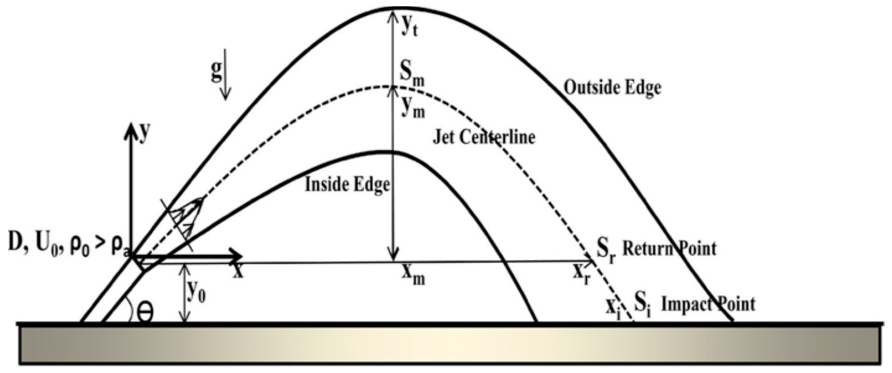Hence, it is important to focus on the near-field region to design the outfall system for greater dilution [7]. Since effluent density varies from the ambient water, which makes the jet rise or fall, when the dense effluent is discharged upwards it is called the negatively buoyant jet. As the jet moves upwards its momentum decreases, which then returns towards the bottom due to its high density after attaining the maximum height. When the effluent’s density is lower than the receiving water, and it is discharged downwards, a penetration depth is attained by the jet and the effluent is therefore made to rise, this is known as a positively buoyant jet [8,9].

Extensive studies have been conducted on negatively buoyant jets. Marti et al. (2010) [7] conducted research, in which an angle of 60 degrees was selected with three different Froude number regimes (one-third, two-thirds, and full-flow capacity) and it was found that the Froude numbers below 20 were giving higher dilution than the predicted extrapolation. Zhang et al. (2016) [10] did the numerical investigation for inclined dense jets at a 45° angle and for the study, a large eddy simulation (LES) method was applied along with a Smagorinsky and Dynamic Smagorinsky sub-grid scale (SGS). Later, numerical results including jet trajectory, geometry, and dilution were cross-validated with the experimental results and it was found that LES was able to regenerate the outputs satisfactorily. Shao and Law (2010) [11] studied the behavior of dense jet for angles of 30° and 45° with different densiometric Froude numbers. For the measurement of velocity and concentration, combined Particle Image Velocimetry (PIV) and Planar Laser-Induced Fluorescence (PLIF) were applied. Velocity and concentration profiles were used to find the mixing and diluting parameters as well. It was found that return point dilution, the horizontal distance of return point, terminal height, centerline peak location, and its dilution were correlated to the Froude number. Oliver et al. (2008) [12] investigated the k-ε turbulence model in the standard fluid dynamics package (CFX) and took two approaches, which included, one with the standard form of the model, and another with a calibrated model achieved by adjusting the Schmidt number. After comparing numerical data, experimental data, along with the data obtained from the studies of previous integral models, concluded that the k-ε model was providing better prediction for the trajectory data, except the data for the integrated dilution at the centerline as they were over-predicting the density gradient, which resulted in the under-estimation of the dilution. Palomar et al. (2012) [13] investigated the performances of CORMIX, VISUAL PLUMES, and VISJET models for the inclined dense studies and obtained some significant differences in the dilution prediction. Kikkert et al. (2007) [14] investigated the behavior of negatively buoyant jets with angles ranging from 0° to 75° and Froude numbers ranging from 14 to 99. The results showed good predictions for the outer spread and the maximum height of the outer edge. However, the inner spread was under-estimated and the minimum dilution prediction was conservative. Along with this, previous studies conducted with CorJet and VisJet models were compared with this study, and it was found that these numerical models had under-predicted the horizontal and vertical locations of maximum jet height. Furthermore, CorJet and VisJet were not accurate enough for an integrated dilution prediction compared to analytical solutions and the data obtained in a study by Kikkert et al. (2007) [14]. Jirka (2008) [15] performed a study with smaller angles, such as 30° and 45°, based on laboratory experiments and numerical modeling using the CorJet model. It was found that the lower angle resulted in higher dilution when the bottom slope was taken into consideration, as it provided better offshore transport of the mixed effluent. Kheirkhah Gildeh et al. (2015) [16] performed numerical modeling with 30° and 45° inclined dense jets. Five CFD models including LRR, RNG k-ε, Realizable k-ε, non-linear k-ε, and Launder Gibson were applied, and it was concluded that LRR and realizable k-ε turbulence models resulted in better predictions for mixing and dilution characteristics.

With the development of computing systems in recent years, the application of combined Fuzzy and AI methods has been increasing in engineering problems. Neshat et al. (2012) [17] used ANFIS models for the optimization of concrete mix designs. They found that the ANFIS model can be better than traditional fuzzy systems and non-fuzzy systems. In a study by Nadia et al. (2020) [18], ANFIS was applied for the prediction of the position of the sun in single- and dual-axis solar tracking systems in an attempt to optimize their performance. The results showed a clear advantage of ANFIS over traditional fuzzy methods with high prediction rates and low error values. Heydary et al. (2021) [19] adopted a combined Fuzzy GMDH (i.e., Group Method of Data Handling) Neural Network and Grey Wolf Optimization (GWO) Algorithm to predict the power produced by wind turbines with consideration of supervisory control and data acquisition (SCADA) data. They first applied a combination of K-means and density-based Local Outliers methods (hybrid K-means-LOF) to remove data outliers and the Empirical Mode Decomposition (EMD) method for the decomposition of SCADA data, and then used the GMDH method to predict the future power generation of wind turbines. They found that the performance of a hybrid EMD-FGMDH-GWO can lead to high accuracy, regardless of the time step applied.

Apart from conventional Computational Fluid Dynamics (CFD) and experimental measurements, soft computing methods could be applied to minimize the computational time for the simulation and investment of money on expensive laboratory equipment. Pourtousi et al. (2015) [20] investigated the combination of the CFD and ANFIS methods for the simulation of bubble column hydrodynamics. Previous experimental data were used to validate the CFD model and later these data were used to train the ANFIS model. It was concluded that ANFIS was a promising method for predicting the outputs of bubble column hydrodynamics. Taghavifar et al. (2015) [21] worked on the assessment of heat accumulation in a hydrogen engine, in which the experimental data were compared with the data obtained after CFD modeling to determine the accuracy between the two. Later, the CFD data were fed an ANFIS code to train the model and it was concluded that the ANFIS model with a Triangular membership function had given the highest R-squared (R²) and lowest root mean squared error (RMSE) value out of other membership functions, and ANFIS was confirmed to be more accurate and simpler than CFD technique in the study. Rezakazemi et al. (2017) [22] evaluated three models, namely ANFIS, ANFIS-PSO, and ANFIS-GA, to determine the performance of hydrogen mixed membranes, in which input parameters such as feed pressure and Nano filter contents were used to evaluate the output parameter (hydrogen gas selectivity). The criteria for investigation of the better model were R² and RMSE values and ANFIS-PSO had given better predictability. Amirkhani et al. (2015) [23] studied the performance of ANN and ANFIS models to estimate the inlet air velocity of the chimney. Three days of experimental data were used to train the models and it was found that the ANFIS model’s results were closer to the experimental results as its R² was higher than ANN. Bonakdari and Zaji (2018) [24] worked on the modified triangular side weir, in which they simulated its discharge coefficient. They studied three different methods of ANFIS, namely ANFIS-GA, ANFIS-PSO, and ANFIS-DE, with combinations of eight different input variables and it was found that ANFIS-DE performed better as it had given lowest the RMSE value compared to ANFIS-GA and ANFIS-PSO. Shabanian et al. (2017) [25] studied the ANFIS model with eight types of membership functions to predict the hydrogen yield of the jet fuel and efficiency of conversion for a non-catalytic filtration combustion reactor. Later, an imperialist competitive algorithm (ICA) was applied to get the optimized results for the hydrogen yield, which was found to be an efficient algorithm for the combustion process optimization. Apart from a soft computing method, multi-gene genetic programming (MCGP) is also a new approach to predict the output, as shown in the study conducted by Yan and Mohammadian (2019) [26], where MCGP turned out to be a promising method for the prediction of vertical buoyant jets.

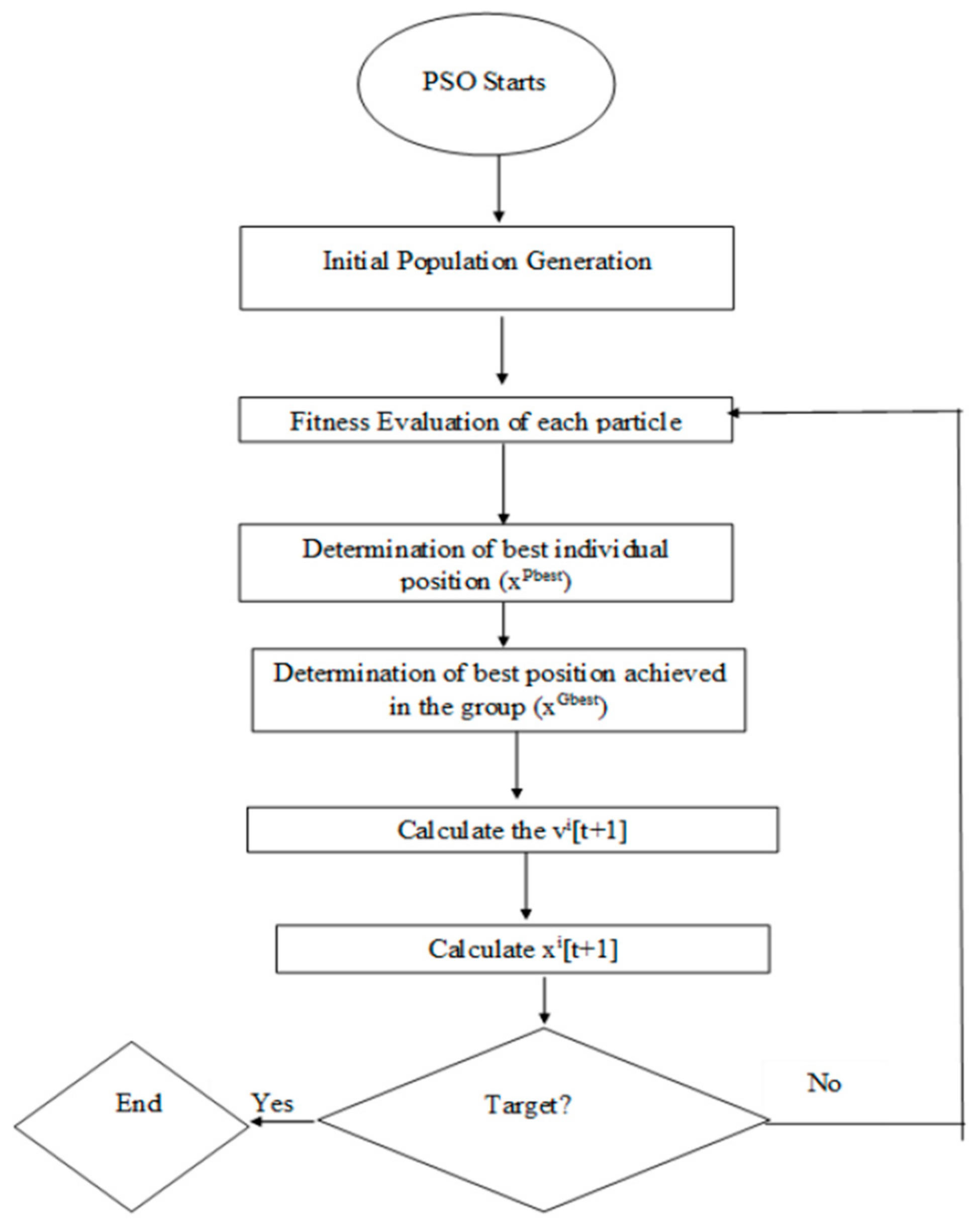
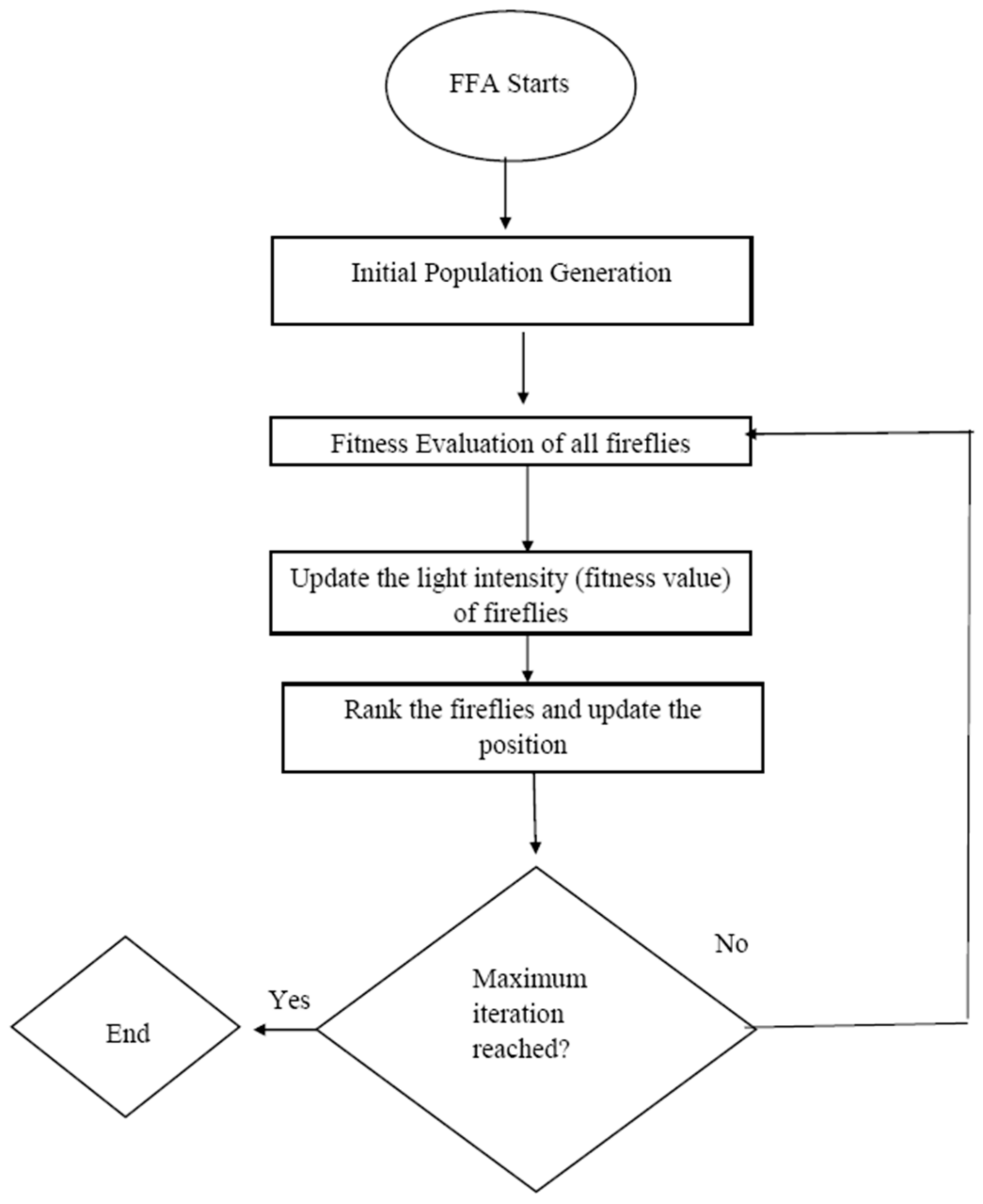
Currently, there is a gap in the application of AI methods in the context of inclined dense jets, which are among the most efficient mixing methods. In particular, to the best of the authors’ knowledge, no previous study has used an ANFIS model and its variants for negatively buoyant jets with an inclination. Such a method can bridge the gap between AI methods and the simulation of inclined dense jets and can potentially simulate these problems more efficiently than CFD methods. The aim of the current study is to consider the application of new AI methods and the generation of data for the testing and training of these models to find the optimum solutions. The main contribution of this project is to apply new AI methods to simulate and predict the dilution of inclined dense jets in the near-field zone. The proposed approach, as shown in this paper, can accurately and efficiently simulate these jets and contribute towards mitigating the negative environmental impacts of such jets. The discharged effluents can create irreversible damage to the marine environment and aquatic life if the outfall systems are not designed properly. The improper design of the system can also leave toxic contaminants in the coastal area. Hence, it is important to design proper outfall systems with efficient mixing. Furthermore, if the concentration of the effluents is determined before their discharge, then it would be helpful in the implementation of the solutions. The salinity of the discharged effluents can either be predicted by experimental or numerical methods, however, to avoid the cost of experimental equipment and save computational time, artificial intelligence techniques can be implemented in the coastal study. The aim of this research is to investigate the application and performance of a soft computing method with ANFIS, ANFIS-GA, ANFIS-PSO, ANFIS-FFA algorithms for negatively buoyant jets to predict the dilution and mixing characteristics. This is the first study on this topic. Negatively buoyant jets are considered for a wide range of Froude numbers, i.e., 5, 10, 12.5, 15, 17.5, 20, 22.5, 25, 27.5, 30, 32.5, 35, 37.5, 40, 50 and 60 with angles ranging from 20 degrees to 72.5 degrees using realizable k-ε model turbulence model in the OpenFOAM platform [27,28].

2. Materials and Methods

2.1. Dimensional Analysis and Numerical Model

As can be seen in Figure 1, negatively buoyant jets are discharged at an angle Θ and velocity U_o, the density of the ambient water is represented by ρ_a, and density of the jet is represented by ρ_o. It can be observed that ρ_o > ρ_a, which makes the jet rise. The diameter of the jet is denoted by D. The terminal height is represented by y_t, which hits the surface at coordinate x_i while the coordinates of peak centerline are represented by x_m and y_m with peak salinity as S_m. Furthermore, jet concentration is represented by C_o. The return point of the jet is represented by x_r and the return salinity value is S_r. For the dimensional analysis a densiometric Froude number is used, which is denoted by the following equation:

$$F{r}_d=\frac{U_{\mathrm{O}}}{\sqrt{g_0^{\prime }D}}$$

(1)

$$g_0^{\prime }=\left(\frac{\mathsf{\Delta }{\rho }_0}{{\rho }_{\mathrm{a}}}\right)$$

(2)

where Δρ_o = (ρ_o − ρ_a) and g₀′ is the reduced gravitational acceleration.

The centerline peak salinity is a function of the Froude number and angle, which can be represented by the following equation:

$$\frac{S_m}{F{r}_d}=f\left(F{r}_{d, } \mathsf{\theta }\right)$$

(3)

For numerical modeling, the following equations were used by Kheirkhah Gildeh et al. (2015) [16]:

• Continuity Equation:

$$\frac{\partial u}{\partial x}+\frac{\partial v}{\partial y}+\frac{\partial w}{\partial z}=0$$

(4)

• Momentum Equations:

$$\frac{\partial u}{\partial t}+u\frac{\partial u}{\partial x}+v\frac{\partial u}{\partial y}+w\frac{\partial u}{\partial z}=-\frac{1}{\rho }\frac{\partial P}{\partial x}+\frac{\partial }{\partial x}\left(v_{\mathrm{eff}}\left(\frac{\partial u}{\partial x}\right)\right)+\frac{\partial }{\partial y}\left(v_{\mathrm{eff}}\left(\frac{\partial u}{\partial y}\right)\right)+\frac{\partial }{\partial z}\left(v_{\mathrm{eff}}\left(\frac{\partial u}{\partial z}\right)\right)$$

(5)

$$\frac{\partial v}{\partial t}+u\frac{\partial v}{\partial x}+v\frac{\partial v}{\partial y}+w\frac{\partial v}{\partial z}=-\frac{1}{\rho }\frac{\partial P}{\partial y}+\frac{\partial }{\partial x}\left(v_{\mathrm{eff}}\left(\frac{\partial v}{\partial x}\right)\right)+\frac{\partial }{\partial y}\left(v_{\mathrm{eff}}\left(\frac{\partial v}{\partial y}\right)\right)+\frac{\partial }{\partial z}\left(v_{\mathrm{eff}}\left(\frac{\partial v}{\partial z}\right)\right)-g\frac{\rho -{\rho }_o}{\rho }$$

(6)

$$\frac{\partial w}{\partial t}+u\frac{\partial w}{\partial x}+v\frac{\partial w}{\partial y}+w\frac{\partial w}{\partial z}=-\frac{1}{\rho }\frac{\partial P}{\partial z}+\frac{\partial }{\partial x}\left(v_{\mathrm{eff}}\left(\frac{\partial w}{\partial x}\right)\right)+\frac{\partial }{\partial y}\left(v_{\mathrm{eff}}\left(\frac{\partial w}{\partial y}\right)\right)+\frac{\partial }{\partial z}\left(v_{\mathrm{eff}}\left(\frac{\partial w}{\partial z}\right)\right)$$

(7)

where v_eff denotes the effective kinematic viscosity, ρ is the fluid density, ρ_o is the reference fluid density and P represents the fluid pressure. Furthermore, the velocity components in x, y, and z directions are represented by u, v, and w.

• Concentration Equation:

$$\frac{\partial C}{\partial t}+u\frac{\partial C}{\partial x}+v\frac{\partial C}{\partial y}+w\frac{\partial C}{\partial z}=D\left(\frac{{\partial }^{2}C}{\partial x^2}+\frac{{\partial }^{2}C}{\partial y^2}+\frac{{\partial }^{2}C}{\partial z^2} \right)$$

(8)

where D is the diffusion coefficient and C denotes the concentration, which in this paper is salinity. For inlet, boundary conditions for velocity in x, y, and z directions are defined as u = U₀ * cos (ɵ), v = U₀ * sin (ɵ) and w = 0. While concentration C = C₀ and Temperature T = T₀ [16].

Initial conditions were assumed as follows: Zero velocity (stagnant) condition was assumed for the flow and the initial concentration of salt was assumed to be zero in the reservoir. As for boundary conditions, a wall function was used for the turbulent quantities at the bottom and a zero-velocity condition (no-slip) was used for the velocity at the bottom wall. Zero shear stress was applied to the top surface and sidewalls, and we developed the condition as assumed for the inlet jet and the values of turbulent quantities such as turbulent kinetic energy and dissipations, which we set according to fully developed pipe flow. The exit of the reservoir was modeled by a zero-gradient condition.

2.2. Data

The data generated from the numerical modeling using the realizable k-ε model in the OpenFOAM platform is used in this part, to train and test the ANFIS and hybrid models. For the soft computing method, two input variables, Froude numbers ranging from 5 to 60 and jet angles ranging from 20 degrees to 72.5, were employed. The aim is to investigate input and output combinations (

Table 1. Input-Output combinations.

Combinations	Input 1	Input 2	Output
1	Froude number	Angle	Sm
2	Froude number	Angle	Sr
3	Froude number	Angle	x
4	Froude number	Angle	xr

) to evaluate the performance of ANFIS, ANFIS-GA, ANFIS-PSO, ANFIS-FFA, and Multivariate regression models. In the present study, the programming language MATLAB is used to design ANFIS [29,30,31], and the three hybrid models, ANFIS-GA [32,33], ANFIS-PSO [33,34], and, ANFIS-FFA [35,36,37]. These models are built on the fundamentals of training and testing, which can be seen in Figure 2. The data are divided into two portions of 70% and 30% for training and model validation, respectively, and various error estimates such as RMSE, R2, etc., are measured for evaluation of the model’s accuracy.

2.3. Adaptive Neuro-Fuzzy Inference System (ANFIS)

Adaptive Neuro-Fuzzy Inference System is an artificial intelligence method, applied to solve nonlinear problems. The architecture for ANFIS containing two inputs, one output, f, and five layers is illustrated in Figure 3. In the architecture, the Sugeno model with Fuzzy IF-THEN rules is employed. The rules R1 and R2 are shown below:

• R1:

$$\mathrm{If} x_1=U_1 \mathrm{and} x_2=V_1$$

(9)

$$\mathrm{Then} f_1=s_1{x}_1+t_1{x}_2+r_1$$

(10)

• R2:

$$\mathrm{If} x_1=U_2 \mathrm{and} x_2=V_2$$

(11)

$$\mathrm{Then} f_2=s_2{x}_1+t_2{x}_2+r_2$$

(12)

where $U_1$, $U_2$ and V₁, V₂ are the membership functions for inputs x₁ and x₂, while s₁, s₂, t₁, t₂, r_1, and r₂ are the adjustable parameters determined during the training process.

The first layer is the input layer, in which input variables are transferred to the next layer and it is formed by the membership functions of the input variables.

$$O_{1,i}={\mu }_{Ui }(x_1), i=1,2$$

(13)

$$O_{1,i}={\mu }_{Vi}\left(x_2\right), i=1,2$$

(14)

The degree of membership functions is represented by ${\mathsf{\mu }}_{Ui}$ and ${\mu }_{Vi}$ for the fuzzy sets U_i and V_i, respectively.

In layer two, each node is fixed and non-adaptive, when each node input values are multiplied by each other, weights (w_i) are obtained.

$$O_{2i}=w_i={\mathsf{\mu }}_{Ui}\left(x_1\right){ \ast \mathsf{\mu }}_{Vi}\left(x_2\right), i=1,2$$

(15)

The third layer, which is non-adaptive in nature, is called the rule layer. In this layer, the weight function is normalized as follows:

$$O_{3i}=w_i^{*}=\frac{w_i}{{{\displaystyle \sum }}_i{w}_i}$$

(16)

The fourth layer, which is the layer where defuzzification takes place and the output of the previous layer, is combined with the Sugeno fuzzy rule’s function. However, nodes in this layer are adaptive and contain a node function:

$$O_{4i}=w_i^{*}{f}_i=w_i^{*}\left(s_i{x}_1+t_i{x}_2+r_i\right)$$

(17)

At layer five, which is the last layer and is called the output layer, the single node will calculate the overall output and will be the summation of all the inputs from the previous layers.

$$O_{5i}={\displaystyle \sum }_i{w}_i^{*}{f}_i=\frac{{{\displaystyle \sum }}_i{w}_i{f}_i}{{{\displaystyle \sum }}_i{w}_i}$$

(18)

2.4. Genetic Algorithm (GA)

Genetic Algorithm [32] is the heuristic search algorithm, which can be classed as an evolutionary algorithm (EA) and is based on the concept of natural selection and genetics, where the idea of inheritance, selection, cross-over, and mutation are applied. It is commonly used in various domains such as manufacturing, engineering, science, etc. [38]. Evolutionary algorithms such as GA are applied in conjugation with ANFIS to enhance the accuracy of the method by finding optimal solutions and lowering errors. The genetic algorithm (GA) starts the process of optimization with a random initial population (Figure 4). In GA, a population is a set of individuals, which are present in the workspace. Each individual has a set of parameters (variables), which are called genes, and are joined together to form a chromosome (solution), which could be mutated and altered. These solutions could either be presented in the form of binary coding, i.e., zeros and ones, or in other encoding forms. The criteria for determining the suitability of individuals are set by an evaluation through fitness function as the population is initialized through randomly generated individuals, hence, it is an iterative process [38]. The best suitable individual with a higher fitness value will be chosen from the population to create the new generation and the solutions of this new generation will be used for the next iteration in the same algorithm. The algorithm will be terminated when the produced generations reach the maximum limit, or a satisfactory fitness level is achieved [38]. In this paper, the GA code has been run in MATLAB software and the ANFIS model has been trained to find the mean salinity S_m, mean coordinates x_m and y_m, return salinity S_r and return coordinates x_r and y_r.

2.5. Particle Swarm Optimization (PSO)

PSO begins with random particles in the search space, which looks for optimal solutions, and each particle is associated with a fitness value, which is evaluated by a fitness function. Each particle is influenced by its best achieved individual position and the best position achieved among the group, and for every iteration, the updating of each particle takes place by these two best values. In every iteration particles choose new velocities based on their current velocity and the two mentioned best values. The new velocity and new position can be evaluated by the following equations [24]:

$$v^{\mathrm{i}}\left[t+1\right]=w{v}^{\mathrm{i}}\left[t\right]+c_1{r}_{1 }\left(x^{\mathrm{Pbest}}\left[t\right]-x^{\mathrm{i}}\left[t\right]\right)+c_2{r}_2\left(x^{\mathrm{Gbest}}\left[t\right]-x^{\mathrm{i}}\left[t\right]\right)$$

(19)

$$x^{\mathrm{i}}\left[t+1\right]=x^{\mathrm{i}}\left[t\right]+v^{\mathrm{i}}\left[t+1\right]$$

(20)

where, xⁱ and vⁱ are the position and velocity vector for particle i and x^Pbest and x^Gbest are the best individual position and best position achieved in the group, respectively. c₁ and c₂ are the personal learning and global learning coefficients, respectively, and r₁ and r₂ are the random coefficients. Furthermore, w represents the inertia weight. The PSO algorithm can be seen in Figure 5.

2.6. Firefly Algorithm (FFA)

The firefly algorithm (FFA) is built on the idea of a relationship between light and fireflies [35]. Based on this relationship, the attractiveness value is directly proportional to the luminosity, hence, it can be calculated by following equations [35,36]:

$$I=I_{\mathrm{o}}{e}^{-\gamma r^2}$$

(21)

$$w\left(r\right)=w_0{e}^{-\gamma r^2}$$

(22)

where w(r) denotes the attractiveness at distance r from the firefly, and I represents the light intensity. I_o and w₀ are the light intensity and attractiveness at distance r = 0 and γ is the coefficient of light absorption [35,36].

The distance between the fireflies i and j is represented by r, and can be calculated from the following equation [35,36]:

$$r_{ij}=\parallel x_{\mathrm{i}}+x_{\mathrm{j}}\parallel =\sqrt{{{\displaystyle \sum }}_{k=1}^d(x_{i,k}}-x_{j,k} )$$

(23)

where x_i and x_j are the locations of fireflies. As fireflies are attracted to one another, the movement for a firefly from one position to another is represented by the following equation [35]:

$${\mathsf{\Delta }}_{xi}={\beta }_0{\mathrm{e}}^{-\gamma r^2}\left(x_{\mathrm{j}}-x_{\mathrm{i}}\right)+\alpha {\epsilon }_i$$

(24)

where α denotes the randomization coefficient and ε_i represents the random number vector. Furthermore, α varies from 0 and 1. ${\beta }_0{\mathrm{e}}^{-\gamma r^2}$ is the attraction term [36]. Figure 6 illustrates the FFA Flowchart.

In this paper, the ANFIS model was integrated with the FFA in order to determine the mean salinity S_m, mean coordinates x_m and y_m, return salinity S_r and return coordinates x_r and y_r. By a trial-and-error method, the values of light absorption coefficient (γ), attraction coefficient base (β₀), and movement coefficient (α) are taken as 0.1, 4, and 0.3, respectively.

2.7. Multivariate Linear Regression Model (MLR)

Multivariate regression analysis is widely used to find a linear relationship between the dependent and multiple independent variables. The data collected from numerical modeling are non-linear, however, to determine the closeness of data with the linearity, multivariate regression analysis has been conducted using Microsoft excel add-ins, which helped to create a model based on least square methods [39]. The generalized equation for MLR can be expressed in the following way [40,41]:

$$Y={\beta }_{\mathrm{o}}+{\beta }_1{X}_1+{\beta }_2{X}_2$$

(25)

where, X₁ and X₂, are the independent variables, which are also called predictor variables. Y is the dependent variable also known as the response variable and n is the number of variables [41].

For multivariate regression, data collected from numerical modeling were divided into training and test data. The equation obtained for the training data set after a regression analysis has been used to generate the predicted test output. The statistical parameters to evaluate the multivariate regression model are the same as the ones used for the ANFIS and hybrid models. The equations mentioned in the statistical parameters section are used for the calculation of the values for regression analysis.

3. Statistical Analysis

To determine the accuracy of ANFIS, ANFIS-GA, ANFIS-PSO, ANFIS-FFA, and multivariate regression models as discussed, statistical parameters of all the models are compared, the statistical parameters taken into consideration are coefficient of determination (R²), root mean squared error (RMSE), mean absolute error (MAE), and average absolute deviation (δ%), i.e., error of the model in percentage [24]. The mentioned parameters can be measured by the following equations:

$$RMSE=\sqrt{\frac{{{\displaystyle \sum }}_{i=1}^N{(O_{\mathrm{i}}-P_{\mathrm{i}})}^2}{N}}$$

(26)

$$R^2=1-\frac{{{\displaystyle \sum }}_{i=1}^N{(O_{\mathrm{i}}-P_{\mathrm{i}})}^2}{{{\displaystyle \sum }}_{i=1}^N{(O_{\mathrm{i}}-O_{\mathrm{m}})}^2}$$

(27)

$$MAE=\frac{1}{N}{{\displaystyle \sum }}_{i=1}^N\mid O_{\mathrm{i}}-P_{\mathrm{i}}\mid$$

(28)

$$\delta \%=\frac{{{\displaystyle \sum }}_{i=1}^N\mid O_{\mathrm{i}}-P_{\mathrm{i}}\mid }{{{\displaystyle \sum }}_{i=1}^N{O}_{\mathrm{i}}}\ast 100$$

(29)

where P_i is the predicted value obtained after training the models, O_i is the observed value obtained after numerical modeling on OpenFOAM, O_m is the mean of observed value and N is the number of samples.

4. Results

Overall, 352 data points are obtained from numerical modeling for each of the S_m, S_r, x, x_r, and y outputs. The data are divided into two sections, training data and test data, where training data contain 272 of the total data and test data contain 80 of the total data test data. For the models, two input variables, i.e., the Froude number and the angle are chosen to obtain one output. The targeted outputs are S, S_r, x_m, y_m, x_r. Hence, five sets with different outputs are prepared for all the models, as shown in Table 1.

4.1. Performance Evaluation for Peak Salinity

The performance of ANFIS-type models and the Multivariate regression model for peak salinity (S_m) is determined in this section.

4.1.1. ANFIS-Type Models

It can be observed from

Table 2. Models’ performance evaluation for S_m.

Model	Output	Training Database				Test Database
		R2	RMSE	MAE	δ%	R2	RMSE	MAE	δ%
ANFIS	Sm	0.9505	0.959	0.726	12.160	0.964	0.890	0.709	11.680
ANFIS-GA	Sm	0.947	1.019	0.834	13.974	0.935	1.187	0.866	14.249
ANFIS-PSO	Sm	0.985	0.547	0.336	5.631	0.984	0.589	0.357	5.889
ANFIS-FFA	Sm	0.979	0.643	0.409	6.866	0.975	0.739	0.447	7.367
Multi-variate Regression	Sm	0.594	2.909	2.118	35.482	0.582	3.009	2.245	36.948

that all the models’ RMSE values for training and test data are almost the same, which means none of them are trapped in over-fitting. Furthermore, in Figure 7a–h, targets and outputs coincide reasonably with each other, which confirms the accuracy of the data for the ANFIS and hybrid models. From Table 2, it can be observed that out of all the models, ANFIS-PSO is giving the highest R², and the lowest RMSE, MAE, and δ%, which are 0.984, 0.589, 0.357, and 5.889% for the test data, making it the most accurate of all.

4.1.2. Multi-Variate Regression Model

The equation obtained after training the regression model for salinity (S_m) is shown below:

$$S_{\mathrm{m}}=13.4212-\left(0.23703\ast Fr\right)-\left(0.01983\ast \mathrm{Angle}\right)$$

(30)

The S_m equation was used to predict the test outputs and it can be seen from Table 2 that in the regression model there is no over-fitted data as the training and test data sets are showing almost similar statistical parameters, however, overall the regression model had the lowest R² value and highest RMSE, MAE and δ %, i.e., in both training and test sets as compared to other models, which made regression model incompatible for predicting peak salinity.

4.2. Performance Evaluation for Return Salinity

The performance of ANFIS-type models and the Multivariate regression model for return salinity (S_r) is determined in this section.

4.2.1. ANFIS-Type Models

Table 3. Models’ performance evaluation for output S_r.

Model	Output	Training Database				Test Database
		R2	RMSE	MAE	δ%	R2	RMSE	MAE	δ%
ANFIS	Sr	0.893	0.923	0.691	23.870	0.909	0.914	0.684	23.028
ANFIS-GA	Sr	0.967	0.510	0.376	12.981	0.976	0.471	0.350	11.803
ANFIS-PSO	Sr	0.958	0.579	0.404	13.946	0.973	0.503	0.395	13.304
ANFIS-FFA	Sr	0.958	0.573	0.369	12.755	0.975	0.481	0.336	11.331
Multi-variate Regression	Sr	0.455	2.147	1.394	48.104	0.441	2.265	1.429	48.077

shows the statistical results for S_r and it can be observed that test data for ANFIS-GA, ANFIS-PSO, and ANFIS-FFA are showing almost the same R² value, i.e., 0.976, 0.973, and 0.975, yet the lowest RMSE was observed in ANFIS-GA, i.e., 0.471. Hence, the ANFIS-GA model can be considered suitable for predicting the return salinity value. Furthermore, the δ% and MAE are also not high for this model. Notably, the RMSE and R² values of the test sets are mainly considered in this thesis work for determining the suitable model.

The graphs in Figure 8a–h shows that targets and outputs are following the same pattern, which again shows that models are properly trained for output S_r.

4.2.2. Multi-Variate Regression Model

The equation obtained after training the regression model for return salinity (S_r) is shown below:

$$S_r=7.601744-\left(0.12495\ast Fr\right)-\left(0.02693\ast \mathrm{Angle}\right)$$

(31)

It can be observed from Table 3 that the parameters for training and test data are almost the same, however, the regression model’s performance compared to other models is very poor, as it has the lowest R² value, i.e., 0.441 and highest RMSE, MAE values, i.e., 2.265 and 1.429 in the test set, respectively, which shows the model accuracy to predict the data is very low and its test outputs are not near to the outputs obtained from the numerical model.

4.3. Performance Evaluation for Peak Coordinate

The performance of ANFIS-type models and Multivariate regression models for peak coordinate (x_m) is determined in this section.

4.3.1. ANFIS-Type Models

From

Table 4. Models’ performance evaluation for output x_m.

Model	Output	Training Database				Test Database
		R2	RMSE	MAE	δ%	R2	RMSE	MAE	δ%
ANFIS	xm	0.985	0.018	0.013	5.409	0.983	0.018	0.013	5.433
ANFIS-GA	xm	0.981	0.020	0.015	6.251	0.987	0.018	0.014	5.736
ANFIS-PSO	xm	0.989	0.015	0.011	4.637	0.976	0.021	0.016	6.250
ANFIS-FFA	xm	0.987	0.017	0.012	5.011	0.987	0.016	0.011	4.650
Multi-Variate Regression	xm	0.899	0.058	0.043	17.707	0.892	0.047	0.036	14.348

, it can be observed that the statistical parameters for output x_m, are showing good accuracy between training and test, which shows none of the models are over-fitted. The models are trained properly, which can be seen from Figure 9a–h. Even though the percentage deviation for ANFIS-FFA’s test data is the smallest out of all the models, the statistical parameters of ANFIS-PSO’s training data are better when compared to its test data, which makes the model more reliable. Furthermore, the test sets for ANFIS-GA and ANFIS-FFA have the highest R², i.e., 0.987, 0.987 with RMSE values, 0.018 and 0.016, respectively. However, considering the RMSE and R² values of the test set, it can be seen that ANFIS-FFA is efficient in determining the output x_m as it has the highest R² and lowest RMSE, though it also has the lowest MAE and δ%.

4.3.2. Multi-Variate Regression Model

To predict, the test output x, the following equation was obtained from the regression analysis of the training set:

$$x_m=0.261093+\left(0.00818\ast Fr\right)-\left(0.00515\ast \mathrm{Angle}\right)$$

(32)

Table 4 shows that although the performance of the regression model was satisfactory, it had the lowest R² value and highest RMSE, MAE, and δ% in the test set compared to the other models’ test sets, which show that the predicted outputs from MLR are not close to the observed numerical outputs. The statistical parameters for the multivariate regression model are calculated by Equations (26)–(29).

4.4. Performance Evaluation for Return Coordinate in x Direction

The performance of ANFIS-type models and the Multivariate regression model for the return coordinate in the x-direction (x_r) is determined in this section.

4.4.1. ANFIS-Type Models

For output x_r,

Table 5. Performance Evaluation for all the models for output x_r.

Model	Output	Training Database				Test Database
		R2	RMSE	MAE	δ%	R2	RMSE	MAE	δ%
ANFIS	xr	0.989	0.028	0.021	4.745	0.981	0.035	0.024	5.119
ANFIS-GA	xr	0.966	0.051	0.039	8.827	0.953	0.056	0.041	8.832
ANFIS-PSO	xr	0.993	0.022	0.016	3.634	0.985	0.032	0.021	4.639
ANFIS-FFA	xr	0.986	0.031	0.023	5.258	0.980	0.035	0.026	5.717
Multi-variate Regression	xr	0.917	0.099	0.076	17.297	0.904	0.079	0.065	13.933

shows all the models’ test data are close in performance to the training data; in fact, the statistical parameters of the training sets are slightly higher than the test sets, which again shows that models are not over-fitted, and they have good predictability, which can be seen in Figure 10a–h. Out of all the models, ANFIS-PSO had given better results as its test set had a higher R² value i.e., 0.985, and lower RMSE, MAE, and δ % i.e., 0.032, 0.021, and 4.639% in the test data, respectively.

4.4.2. Multi-Variate Regression Model

For output x_r, the multivariate regression model showed quite good results with R² as 0.9044, and RMSE, MAE values as 0.079 and 0.065, respectively. The percentage deviation between the observed and predicted test output was 13.93%. The equation used for the predicted output was:

$$x_{\mathrm{r}}=0.399753+\left(0.015318\ast Fr\right)-\left(0.00804\ast \mathrm{Angle}\right)$$

(33)

4.5. Performance Evaluation for Peak Coordinate in y Direction

The performance of ANFIS-type models and the Multivariate regression model for the peak coordinate in the y-direction (y_m) is determined in this section.

4.5.1. ANFIS-Type Models

From

Table 6. Models’ performance evaluation for output y_m.

Model	Output	Training Database				Test Database
		R2	RMSE	MAE	δ%	R2	RMSE	MAE	δ%
ANFIS	ym	0.985	0.014	0.010	5.014	0.989	0.013	0.010	5.157
ANFIS-GA	ym	0.979	0.017	0.012	6.093	0.979	0.019	0.014	7.472
ANFIS-PSO	ym	0.990	0.011	0.008	3.900	0.986	0.014	0.010	5.285
ANFIS-FFA	ym	0.981	0.016	0.011	5.4363	0.986	0.014	0.010	5.475
Multivariate Regression	ym	0.855	0.040	0.030	15.016	0.846	0.049	0.038	19.735

it can be seen that the percentage deviations for both the data sets in ANFIS-GA are 6.093% and 7.472%, which are higher than all the ANFIS-type models. However, ANFIS, ANFIS-PSO, and ANFIS-FFA had given similar R² values, i.e., 0.989, 0.986, 0.986, respectively, for their test data sets, which are highest in the test data for all the models. Also, their test sets R² value is comparable to their respective training set, which shows the models are trained properly. Along with this, the RMSE values for ANFIS, ANFIS-PSO, ANFIS-FFA are 0.013, 0.014, 0.014, respectively, with the same MAE value of 0.010. Hence, they can be considered for the prediction of y_m. Figure 11a–h shows that models are not over-fitted as targets and outputs coincide with each other.

4.5.2. Multivariate Regression

The equation obtained after the regression analysis on the training set to obtain the predicted test outputs is:

$$y_{\mathrm{m}}=-0.13746+\left(0.007027\ast Fr\right)+\left(0.003153\ast \mathrm{Angle}\right)$$

(34)

It can be deduced from Table 6 that training and test sets show good similarity with each other, which proves that the data is not over-fitted and that statistical parameters’ values are lower as compared to ANFIS and hybrid ANFIS models. The gap between the predicted test output and observed test output is visible by the percentage deviation of 19.735%.

5. Discussion

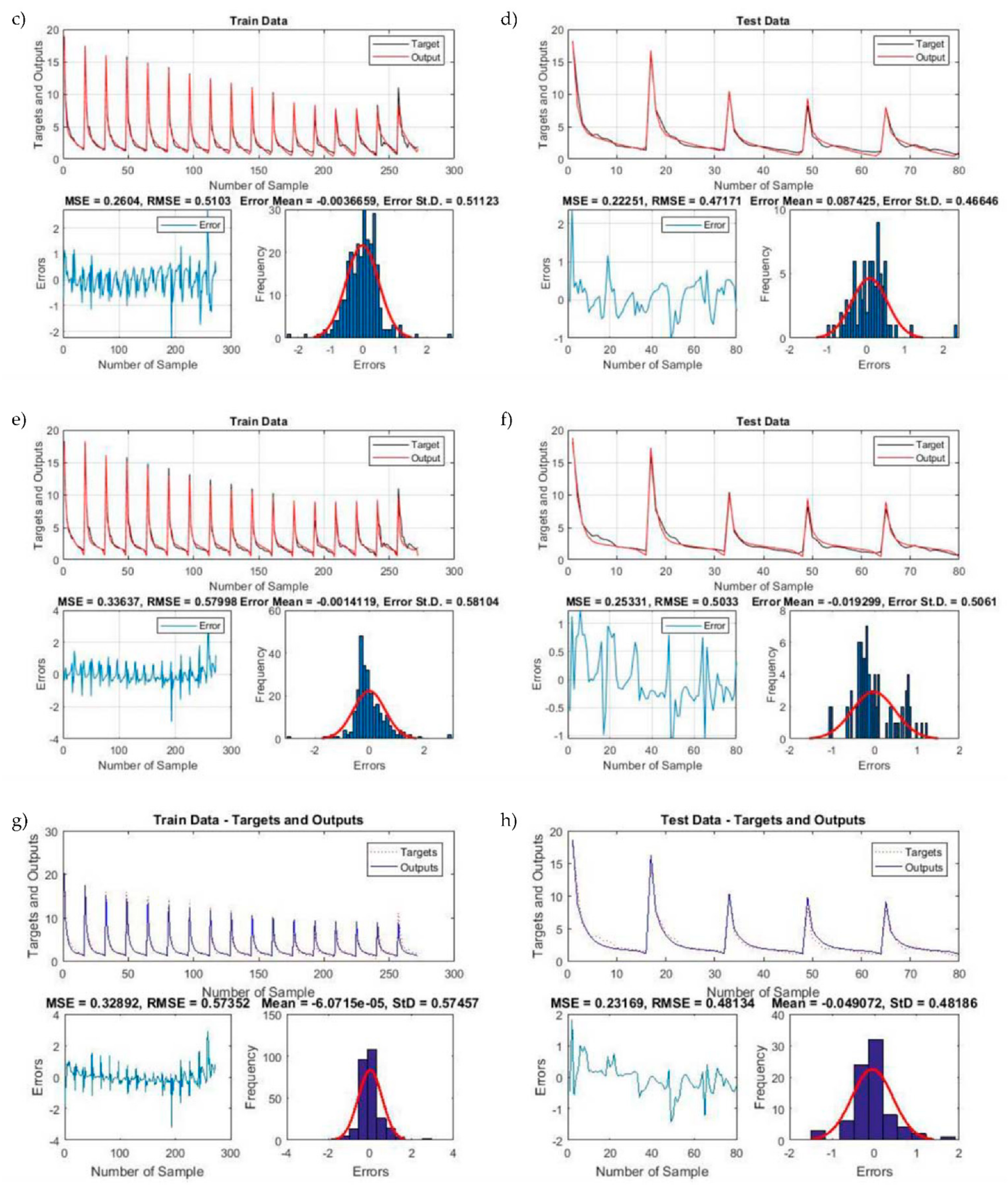
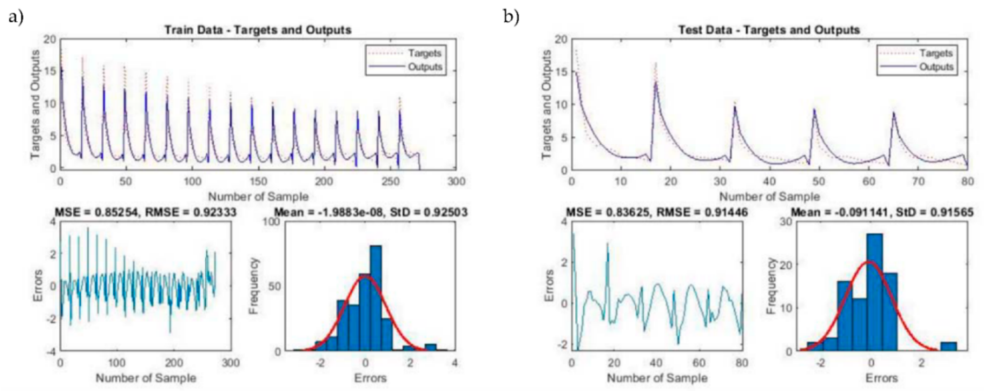
In this paper, the ANFIS model was incorporated with three different algorithms, namely, the Genetic Algorithm, Particle Swarm Optimization, and Firefly Algorithm. Also, to check the linearity of the data, a multivariate linear regression (MLR) was conducted. It was found that the coefficient of determination was too low for MLR, and root mean squared error (RMSE) was too high compared to ANFIS and hybrid ANFIS models. Four statistical indices were measured to determine the efficient model, and they were the coefficient of determination, root mean squared error, mean absolute error, and percentage deviation. Furthermore, to determine the reliable model, the statistical indices of the test set were compared for all the models. It could be seen that, for all the ANFIS-type models, over-fitting was not observed, which showed the models were trained well.

For different outputs, different models showed accuracy. Hence, to evaluate the overall model performance, the average of all the statistical parameters needs to be calculated. It could be seen from

Table 7. Overall performance evaluation for all the test data outputs.

Model	Training Set				Test Set
	R2	RMSE	MAE	δ%	R2	RMSE	MAE	δ%
ANFIS	0.960	0.388	0.292	10.239	0.965	0.374	0.288	10.083
ANFIS-GA	0.968	0.323	0.255	9.625	0.966	0.350	0.257	9.618
ANFIS-PSO	0.983	0.234	0.155	6.349	0.980	0.231	0.159	7.073
ANFIS-FFA	0.978	0.256	0.164	7.065	0.980	0.257	0.166	6.908
Multivariate Regression	0.744	1.051	0.732	26.721	0.733	1.090	0.762	26.608

that ANFIS-PSO and ANFIS-FFA generated the same value for R², i.e., 0.980. Also, the RMSE values of these models are lower than the rest of the models, i.e., 0.231 and 0.257, respectively. It could also be seen that the training data of ANFIS-PSO is better compared to ANFIS-FFA as the training set of ANFIS-PSO’s R² value was 0.983. The model, which showed the poor performance, was MLR as it had the lowest R² value, i.e., 0.733, and highest RMSE value, i.e., 1.090. The present study will be helpful in coastal research worldwide it is one of the first studies on artificial intelligence models in negatively buoyant jets for predicting effluent discharges in less computational time as the computational fluid dynamic model had taken approximately three and half days for simulation compared to the ANFIS-type models, which had taken ten to fifteen minutes.

Additionally, as AI techniques are widely used in the majority of sectors worldwide, it would be interesting to see their implementation in coastal studies. Most of the previous studies have been conducted using computational fluid dynamics models, and this is one of the first studies to have implemented artificial intelligence models in negatively buoyant jets. The study is also an extension of the Kheirkhah Gildeh et al. (2015) [16] study and it can be seen that the ANFIS-type models have performed as well as the CFD model, with less computational time. Although, as mentioned earlier, the present study is one of the first studies using AI models in coastal systems, there are some studies conducted on different coastal topics such as the Bonakdari and Zaji (2018) [24] study on the side weir discharge coefficient, which was modeled using ANFIS-type models. Yan and Mohammadian (2019) [26] studied the Multi-Gene Genetic Programming (MGGP) method for vertical buoyant jets to determine dilution properties. The approach, MGGP in this study, was efficient and accurate, hence, it can also be used to examine the present study on negatively buoyant jets for future work. Furthermore, in future work, several different algorithms such as Differential Evolution (DE), Ant Colony (ACO), Cuckoo Optimization Algorithm (COA) could also be merged with ANFIS to broaden the area of negatively buoyant jet study.

Furthermore, parameters such as temperature, sloping bed, density current, rosette diffuser, effects of stratification on various types of discharges with or without current, effects of secondary flow, various types of jets under wave effect, or current effect can also be considered. Other statistical parameters such as Scatter Index, BIAS, Nash, VAF can also be checked for performance evaluation. Along with this, positive and negative jets can be examined for crossflow using various AI methods such as ANFIS type procedures.

As the errors and performance results in Table 7 show, hybrid models such as ANFIS-PSO and ANFIS-FFA, in comparison with ANFIS, present lower error estimates and overall, more accurate solutions. However, the hybrid models have a higher computational cost. Therefore, the application of these models depends on the desired accuracy and the availability of computing systems. In other words, there is no single answer as to which model is to be selected.

It should be noted that this project did not attempt to train the model and validate it using real-time data, which is the subject of a subsequent study, in order to extend the use of the model to more practical applications.

6. Conclusions

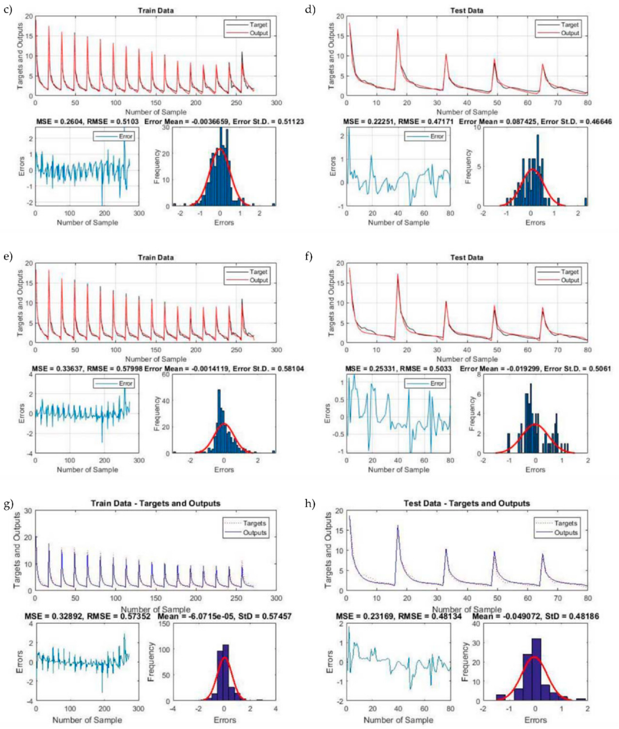
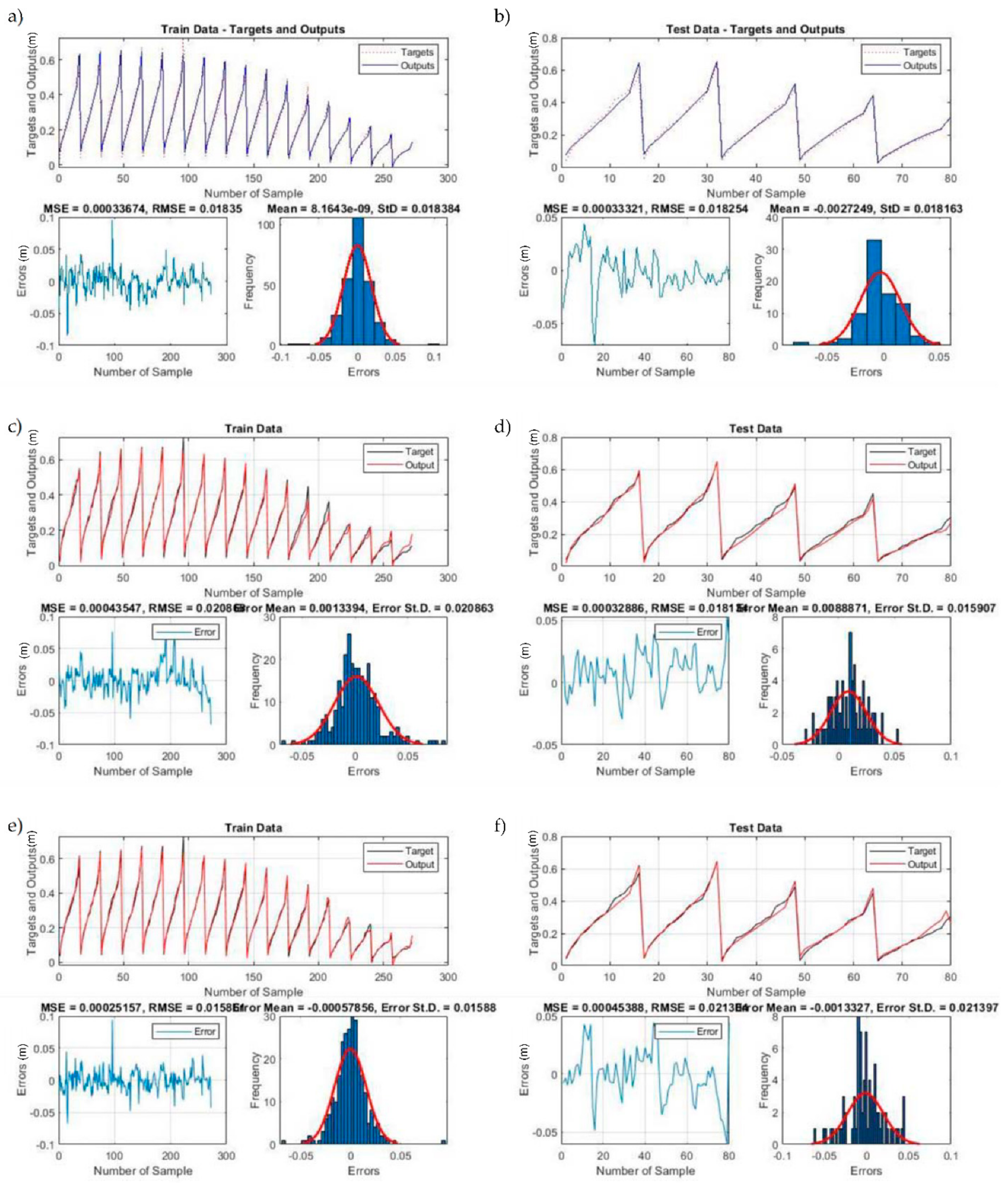
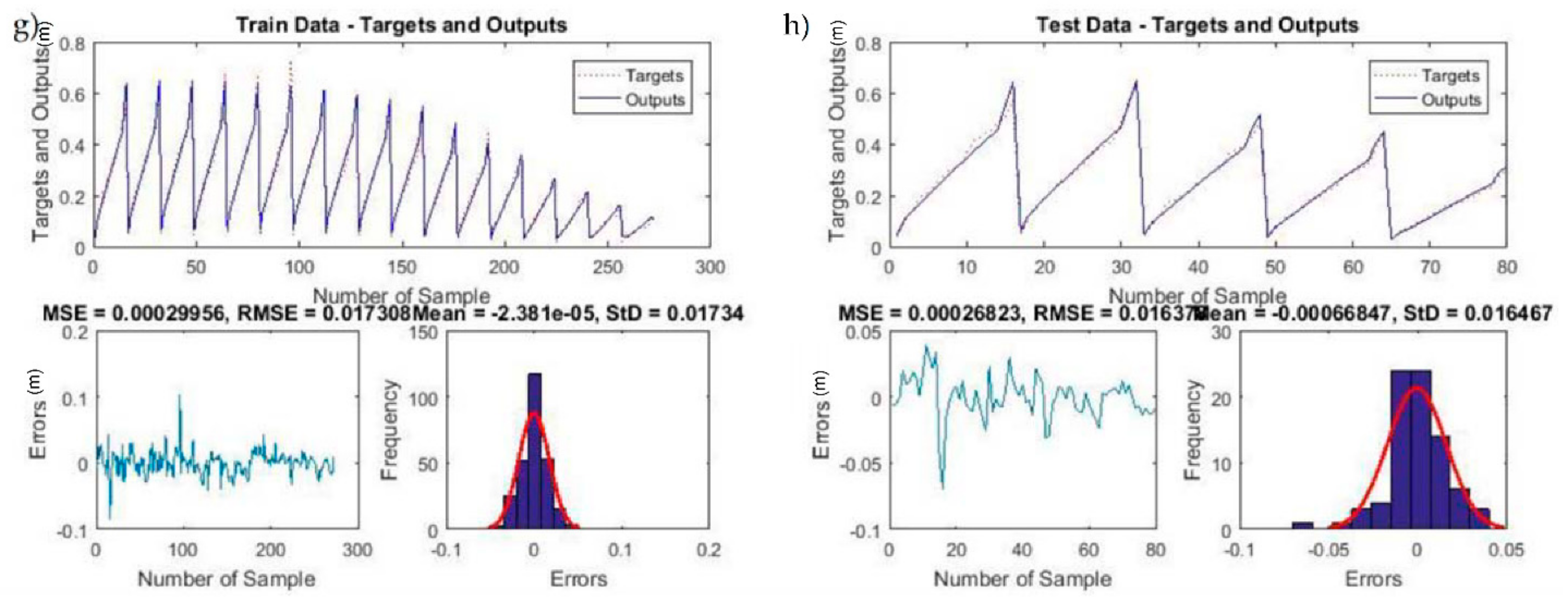
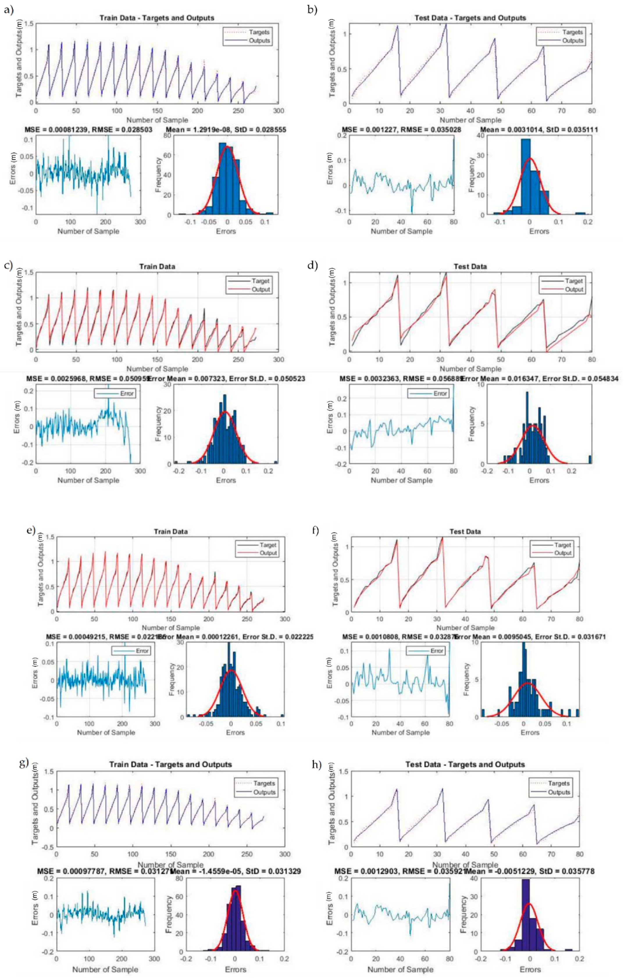
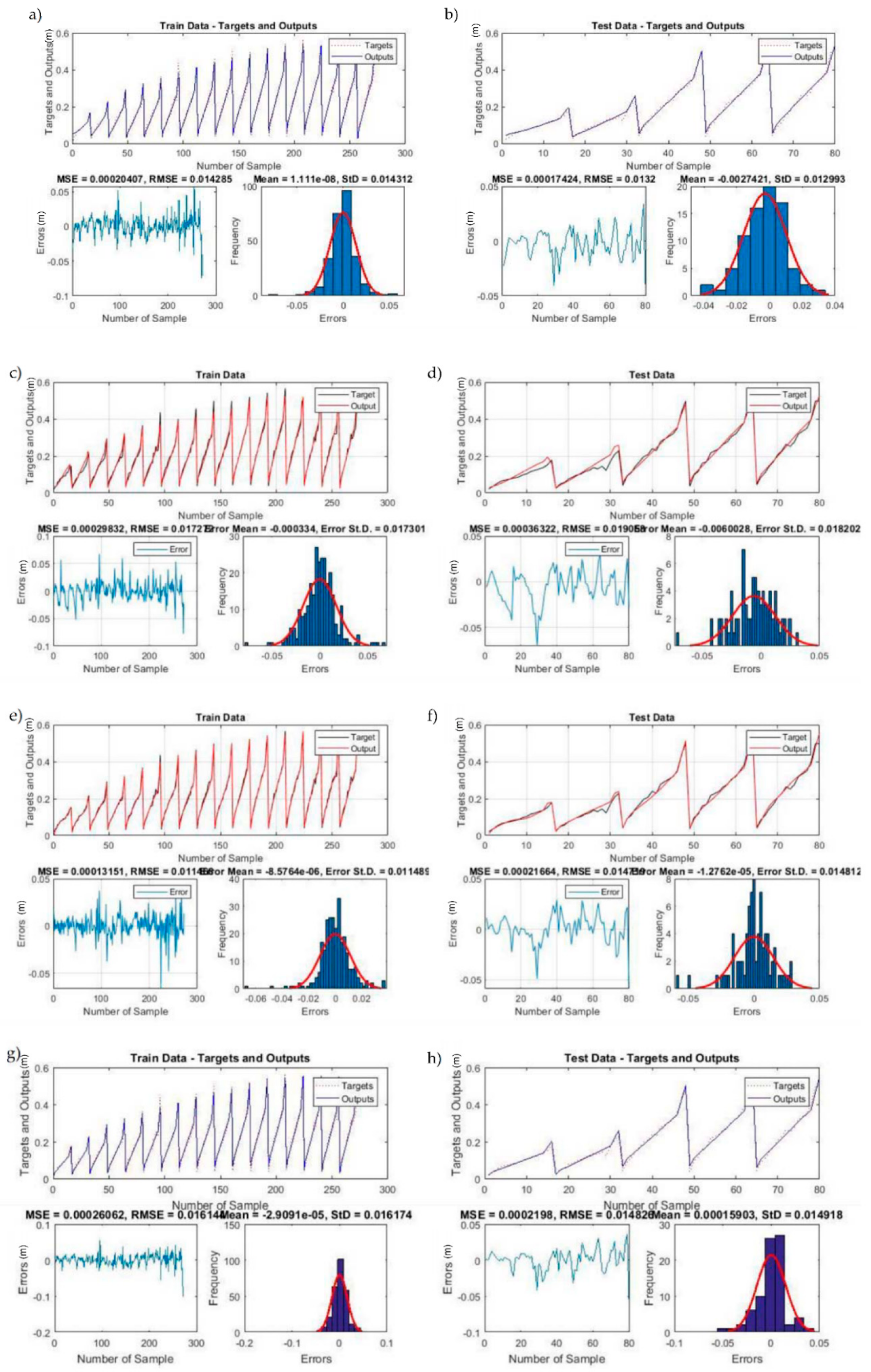
ANFIS model alone and different hybrid models such as ANFIS-GA, ANFIS-PSO, and ANFIS-FFA along with multivariate regression were investigated for the prediction of industrial outfall discharges. In this paper, negatively buoyant jets are focused. Proper outfall design is one of the important factors to mitigate the environmental effects of effluent discharge from desalination plants. With prior knowledge of effluents’ discharge characteristics, it is easier to implement proper solutions. Though most of the studies have been conducted using experimental and numerical methods, in this study, the ANFIS type models are examined for lesser computational time and to avoid the cost of an experimental setup. The results showed that ANFIS and hybrid models were trained properly, which could be seen from targets and output graphs in Figure 2, Figure 3, Figure 4, Figure 5, Figure 6, Figure 7, Figure 8, Figure 9, Figure 10 and Figure 11 as they almost coincided with each other. However, the results showed that the multi-variate regression model was not successful in interpreting the relationship between independent and dependent variables, especially due to the non-linearity of the data. Hence, ANFIS and hybrid models are suitable choices to predict the dilution characteristics of outfall discharges. To determine the efficient model to predict all the outputs mentioned in the previous section, it can be deduced from Table 7, which is generated by averaging all the outputs that ANFIS-PSO has the highest R² value, lowest RMSE, and lowest MAE. The other model which showed the same R² value to ANFIS-PSO is ANFIS-FFA, however, its RMSE value and MAE value are 0.257 and 0.166, respectively, which are a little higher than ANFIS-PSO. Furthermore, the difference observed between ANFIS-PSO and ANFIS-FFA was in their computational time, which was more for ANFIS-FFA at around 3.5 h compared to ANFIS-PSO, which was 10–15 min. Although, the computational time for all the ANFIS-type models was much less compared to the CFD model, which was approximately around 3.5 days. Overall, these two models, ANFIS-FFA and ANFIS-PAO, can be considered suitable for predicting the effluent discharge, although ANFIS-PSO would be preferable when one considers computational cost as a deciding factor.

The results presented in Table 7 demonstrate that hybrid models (especially ANFIS-PSO and ANFIS-FSA) overall, provide better results with lower errors than ANFIS. However, if one is looking for a quicker answer, ANFIS alone provides results within an acceptable margin of error and can be used.

The use of real-time data for training and validation of the model can be examined in a future study to enhance the practical applicability of the model.

References

1. Purnama, A.; Shao, D. Modeling brine discharge dispersion from two adjacent desalination outfalls in coastal waters. Desalination 2015, 362, 68–73. [Google Scholar] [CrossRef]
2. Alameddine, I.; El-Fadel, M. Brine discharge from desalination plants: A modeling approach to an optimized outfall design. Desalination 2007, 214, 241–260. [Google Scholar] [CrossRef]
3. Termeh, S.V.R.; Khosravi, K.; Sartaj, M.; Keesstra, S.D.; Tsai, F.T.C.; Dijksma, R.; Pham, B.T. Optimization of an adaptive neuro-fuzzy inference system for groundwater potential mapping. Hydrogeol. J. 2019, 27, 2511–2534. [Google Scholar] [CrossRef]
4. Bleninger, T.; Jirka, G.H. Modelling and environmentally sound management of brine discharges from desalination plants. Desalination 2008, 221, 585–597. [Google Scholar] [CrossRef]
5. Christodoulou, G.C.; Papakonstantis, I.G.; Nikiforakis, I.K. Desalination brine disposal by means of negatively buoyant jets. Desalin. Water Treat. 2015, 53, 3208–3213. [Google Scholar] [CrossRef]
6. Malcangio, D.; Petrillo, A.F. Modeling of brine outfall at the planning stage of desalination plants. Desalination 2010, 254, 114–125. [Google Scholar] [CrossRef]
7. Marti, C.L.; Antenucci, J.P.; Luketina, D.; Okely, P.; Imberger, J. Near-field dilution characteristics of a negatively buoyant hypersaline jet generated by a desalination plant. J. Hydraul. Eng. 2010, 137, 57–65. [Google Scholar] [CrossRef] [Green Version]
8. Papakonstantis, I.G.; Christodoulou, G.C.; Papanicolaou, P.N. Inclined negatively buoyant jets 1: Geometrical characteristics. J. Hydraul. Res. 2011, 49, 3–12. [Google Scholar] [CrossRef]
9. Papakonstantis, I.G.; Christodoulou, G.C.; Papanicolaou, P.N. Inclined negatively buoyant jets 2: Concentration measurements. J. Hydraul. Res. 2011, 49, 13–22. [Google Scholar] [CrossRef]
10. Zhang, S.; Jiang, B.; Law, A.W.K.; Zhao, B. Large eddy simulations of 45 inclined dense jets. Environ. Fluid Mech. 2016, 16, 101–121. [Google Scholar] [CrossRef]
11. Shao, D.; Law, A.W.K. Mixing and boundary interactions of 30 and 45 inclined dense jets. Environ. Fluid Mech. 2010, 10, 521–553. [Google Scholar] [CrossRef]
12. Oliver, C.J.; Davidson, M.J.; Nokes, R.I. k-ε Predictions of the initial mixing of desalination discharges. Environ. Fluid Mech. 2008, 8, 617. [Google Scholar] [CrossRef]
13. Palomar, P.; Lara, J.L.; Losada, I.J. Near field brine discharge modeling part 2: Validation of commercial tools. Desalination 2012, 290, 28–42. [Google Scholar] [CrossRef]
14. Kikkert, G.A.; Davidson, M.J.; Nokes, R.I. Inclined negatively buoyant discharges. J. Hydraul. Eng. 2007, 133, 545–554. [Google Scholar] [CrossRef]
15. Jirka, G.H. Improved discharge configurations for brine effluents from desalination plants. J. Hydraul. Eng. 2008, 134, 116–120. [Google Scholar] [CrossRef] [Green Version]
16. Kheirkhah Gildeh, H.; Mohammadian, A.; Nistor, I.; Qiblawey, H. Numerical modeling of 30° and 45° inclined dense turbulent jets in stationary ambient. Environ. Fluid Mech. 2015, 15, 537–562. [Google Scholar] [CrossRef]
17. Neshat, M.; Adeli, A.; Sepidnam, G.; Sargolzaei, M. Predication of concrete mix design using adaptive neural fuzzy inference systems and fuzzy inference systems. Int. J. Adv. Manuf. Technol. 2012, 63, 373–390. [Google Scholar] [CrossRef]
18. Nadia, A.R.; Isa, N.A.M.; Desa, M.K.M. Efficient single and dual axis solar tracking system controllers based on adaptive neural fuzzy inference system. J. King Saud Univ. Eng. Sci. 2020, 32, 459–469. [Google Scholar]
19. Heydari, A.; Majidi Nezhad, M.; Neshat, M.; Garcia, D.A.; Keynia, F.; De Santoli, L.; Tjernberg, L.B. A combined fuzzy GMDH neural network and grey wolf optimization application for wind turbine power production forecasting considering SCADA data. Energies 2021, 14, 3459. [Google Scholar] [CrossRef]
20. Pourtousi, M.; Sahu, J.N.; Ganesan, P.; Shamshirband, S.; Redzwan, G. A combination of computational fluid dynamics (CFD) and adaptive neuro-fuzzy system (ANFIS) for prediction of the bubble column hydrodynamics. Powder Technol. 2015, 274, 466–481. [Google Scholar] [CrossRef]
21. Taghavifar, H.; Khalilarya, S.; Jafarmadar, S. Adaptive neuro-fuzzy system (ANFIS) based appraisal of accumulated heat from hydrogen-fueled engine. Int. J. Hydrog. Energy 2015, 40, 8206–8218. [Google Scholar] [CrossRef]
22. Rezakazemi, M.; Dashti, A.; Asghari, M.; Shirazian, S. H2-selective mixed matrix membranes modeling using ANFIS, PSO-ANFIS, GA-ANFIS. Int. J. Hydrog. Energy 2017, 42, 15211–15225. [Google Scholar] [CrossRef]
23. Amirkhani, S.; Nasirivatan, S.; Kasaeian, A.B.; Hajinezhad, A. ANN and ANFIS models to predict the performance of solar chimney power plants. Renew. Energy 2015, 83, 597–607. [Google Scholar] [CrossRef]
24. Bonakdari, H.; Zaji, A.H. New type side weir discharge coefficient simulation using three novel hybrid adaptive neuro-fuzzy inference systems. Appl. Water Sci. 2018, 8, 10. [Google Scholar] [CrossRef] [Green Version]
25. Shabanian, S.R.; Edrisi, S.; Khoram, F.V. Prediction and optimization of hydrogen yield and energy conversion efficiency in a non-catalytic filtration combustion reactor for jet A and butanol fuels. Korean J. Chem. Eng. 2017, 34, 2188–2197. [Google Scholar] [CrossRef]
26. Yan, X.; Mohammadian, A. Multigene Genetic-Programming-Based Models for Initial Dilution of Laterally Confined Vertical Buoyant Jets. J. Mar. Sci. Eng. 2019, 7, 246. [Google Scholar] [CrossRef] [Green Version]
27. OpenFOAM Version 2.3.1. Computer Software. Available online: https://openfoam.org/version/2-3-1/ (accessed on 7 January 2022).
28. Greenshields, C.J. OpenFOAM User Guide; The OpenFOAM Foundation: London, UK, 2018. [Google Scholar]
29. Jang, J.S. ANFIS: Adaptive-network-based fuzzy inference system. IEEE Trans. Syst. Man Cybern. 1993, 23, 665–685. [Google Scholar] [CrossRef]
30. Ebtehaj, I.; Bonakdari, H. Performance evaluation of adaptive neural fuzzy inference system for sediment transport in sewers. Water Resour. Manag. 2014, 28, 4765–4779. [Google Scholar] [CrossRef]
31. Bonakdari, H.; Zaji, A.H.; Shamshirband, S.; Hashim, R.; Petkovic, D. Sensitivity analysis of the discharge coefficient of a modified triangular side weir by adaptive neuro-fuzzy methodology. Measurement 2015, 73, 74–81. [Google Scholar] [CrossRef]
32. Holland, J. Adaptation in Natural and Artificial Systems: An Introductory Analysis with Applications to Biology, Control, and Artificial Intelligence; MIT Press: Cambridge, MA, USA, 1975. [Google Scholar]
33. Yarpiz Evolutionary Algorithms. Available online: https://yarpiz.com/477/ypea-yarpiz-evolutionary-algorithms (accessed on 7 January 2022).
34. Kennedy, J.; Eberhart, R. Particle swarm optimization (PSO). In Proceedings of the IEEE International Conference on Neural Networks, Perth, Australia, 27 November–1 December 1995; pp. 1942–1948. [Google Scholar]
35. Yang, X.S. Firefly algorithm, Levy flights and global optimization. In Research and Development in Intelligent Systems XXVI; Springer: London, UK, 2010; pp. 209–218. [Google Scholar]
36. Yaseen, Z.M.; Ebtehaj, I.; Bonakdari, H.; Deo, R.C.; Mehr, A.D.; Mohtar, W.H.M.W.; Diop, L.; El-Shafie, A.; Singh, V.P. Novel approach for streamflow forecasting using a hybrid ANFIS-FFA model. J. Hydrol. 2017, 554, 263–276. [Google Scholar] [CrossRef]
37. Azimi, H.; Bonakdari, H.; Ebtehaj, I.; Michelson, D.G. A combined adaptive neuro-fuzzy inference system–firefly algorithm model for predicting the roller length of a hydraulic jump on a rough channel bed. Neural Comput. Appl. 2018, 29, 249–258. [Google Scholar] [CrossRef]
38. Yaghoobi, A.; Bakhshi-Jooybari, M.; Gorji, A.; Baseri, H. Application of adaptive neuro fuzzy inference system and genetic algorithm for pressure path optimization in sheet hydroforming process. Int. J. Adv. Manuf. Technol. 2016, 86, 2667–2677. [Google Scholar] [CrossRef]
39. Emadi, D.; Mahfoud, M. Comparison of Artificial Neural Network and Multiple Regression Analysis Techniques in Predicting the Mechanical Properties of A356 Alloy. Procedia Eng. 2011, 10, 589–594. [Google Scholar] [CrossRef] [Green Version]
40. Tosun, E.; Aydin, K.; Bilgili, M. Comparison of linear regression and artificial neural network model of a diesel engine fueled with biodiesel-alcohol mixtures. Alex. Eng. J. 2016, 55, 3081–3089. [Google Scholar] [CrossRef] [Green Version]
41. Fumo, N.; Biswas, M.R. Regression analysis for prediction of residential energy consumption. Renew. Sustain. Energy Rev. 2015, 47, 332–343. [Google Scholar] [CrossRef]
Figure 1. Configuration for Negatively Buoyant Jet (Reprinted with permission from Ref. [16]. Copyright 2022 Springer Nature).
Mca 27 00029 g001
Figure 2. Training data and Test.
Mca 27 00029 g002
Figure 3. ANFIS structure.
Mca 27 00029 g003
Figure 4. GA Flowchart.
Mca 27 00029 g004
Figure 5. PSO Flowchart.
Mca 27 00029 g005
Figure 6. FFA Flowchart.
Mca 27 00029 g006
Figure 7. For output Sm, ANFIS Model (a) targets and outputs, RMSE, MSE values and frequency vs. errors graphs for train data set (b) targets and outputs, RMSE, MSE values and frequency vs. errors graphs for test data set. ANFIS-GA: (c) targets and outputs, RMSE, MSE values and frequency vs. errors graphs for train data set (d) targets and outputs, RMSE, MSE values, and frequency vs. errors graphs for test data set. ANFIS-PSO: (e) targets and outputs, RMSE, MSE values and frequency vs. errors for train data set (f) targets and outputs, RMSE, MSE values, and frequency vs. errors for test data set. ANFIS-FFA: (g) targets and outputs, RMSE, MSE values and frequency vs. errors for train data set (h) targets and outputs, RMSE, MSE values, and frequency vs. errors for test data set.
Mca 27 00029 g007aMca 27 00029 g007b
Figure 8. For output Sr, ANFIS Model (a) targets and outputs, RMSE, MSE values and frequency vs. errors graphs for train data set (b) targets and outputs, RMSE, MSE values and frequency vs. errors graphs for test data set. ANFIS-GA: (c) targets and outputs, RMSE, MSE values and frequency vs. errors graphs for train data set (d) targets and outputs, RMSE, MSE values, and frequency vs. errors graphs for test data set. ANFIS-PSO: (e) targets and outputs, RMSE, MSE values and frequency vs. errors for train data set (f) targets and outputs, RMSE, MSE values, and frequency vs. errors for test data set. ANFIS-FFA: (g) targets and outputs, RMSE, MSE values and frequency vs. errors for train data set (h) targets and outputs, RMSE, MSE values, and frequency vs. errors for test data set.
Mca 27 00029 g008aMca 27 00029 g008b
Figure 9. For output xm, ANFIS Model (a) targets and outputs, RMSE, MSE values and frequency vs. errors graphs for train data set (b) targets and outputs, RMSE, MSE values and frequency vs. errors graphs for test data set. ANFIS-GA: (c) targets and outputs, RMSE, MSE values and frequency vs. errors graphs for train data set (d) targets and outputs, RMSE, MSE values, and frequency vs. errors graphs for test data set. ANFIS-PSO: (e) targets and outputs, RMSE, MSE values and frequency vs. errors for train data set (f) targets and outputs, RMSE, MSE values, and frequency vs. errors for test data set. ANFIS-FFA: (g) targets and outputs, RMSE, MSE values and frequency vs. errors for train data set (h) targets and outputs, RMSE, MSE values, and frequency vs. errors for test data set.
Mca 27 00029 g009aMca 27 00029 g009b
Figure 10. For output xr, ANFIS Model (a) targets and outputs, RMSE, MSE values and frequency vs. errors graphs for train data set (b) targets and outputs, RMSE, MSE values and frequency vs. errors graphs for test data set. ANFIS-GA: (c) targets and outputs, RMSE, MSE values and frequency vs. errors graphs for train data set (d) targets and outputs, RMSE, MSE values, and frequency vs. errors graphs for test data set. ANFIS-PSO: (e) targets and outputs, RMSE, MSE values and frequency vs. errors for train data set (f) targets and outputs, RMSE, MSE values, and frequency vs. errors for test data set. ANFIS-FFA: (g) targets and outputs, RMSE, MSE values and frequency vs. errors for train data set (h) targets and outputs, RMSE, MSE values, and frequency vs. errors for test data set.
Mca 27 00029 g010
Figure 11. As in Figure 9 for ym. ANFIS Model (a) targets and outputs, RMSE, MSE values and frequency vs. errors graphs for train data set (b) targets and outputs, RMSE, MSE values and frequency vs. errors graphs for test data set. ANFIS-GA: (c) targets and outputs, RMSE, MSE values and frequency vs. errors graphs for train data set (d) targets and outputs, RMSE, MSE values, and frequency vs. errors graphs for test data set. ANFIS-PSO: (e) targets and outputs, RMSE, MSE values and frequency vs. errors for train data set (f) targets and outputs, RMSE, MSE values, and frequency vs. errors for test data set. ANFIS-FFA: (g) targets and outputs, RMSE, MSE values and frequency vs. errors for train data set (h) targets and outputs, RMSE, MSE values, and frequency vs. errors for test data set.
Mca 27 00029 g011