Evaluation of Machine Learning Algorithms for Early Diagnosis of Deep Venous Thrombosis

Abstract

Deep venous thrombosis (DVT) is a disease that must be diagnosed quickly, as it can trigger the death of patients. Nowadays, one can find different ways to determine it, including clinical scoring, D-dimer, ultrasonography, etc. Recently, scientists have focused efforts on using machine learning (ML) and neural networks for disease diagnosis, progressively increasing the accuracy and efficacy. Patients with suspected DVT have no apparent symptoms. Using pattern recognition techniques, aiding good timely diagnosis, as well as well-trained ML models help to make good decisions and validation. The aim of this paper is to propose several ML models for a more efficient and reliable DVT diagnosis through its implementation on an edge device for the development of instruments that are smart, portable, reliable, and cost-effective. The dataset was obtained from a state-of-the-art article. It is divided into 85% for training and cross-validation and 15% for testing. The input data in this study are the Wells criteria, the patient’s age, and the patient’s gender. The output data correspond to the patient’s diagnosis. This study includes the evaluation of several classifiers such as Decision Trees (DT), Extra Trees (ET), K-Nearest Neighbor (KNN), Multi-Layer Perceptron Neural Network (MLP-NN), Random Forest (RF), and Support Vector Machine (SVM). Finally, the implementation of these ML models on a high-performance embedded system is proposed to develop an intelligent system for early DVT diagnosis. It is reliable, portable, open source, and low cost. The performance of different ML algorithms was evaluated, where KNN achieved the highest accuracy of 90.4% and specificity of 80.66% implemented on personal computer (PC) and Raspberry Pi 4 (RPi4). The accuracy of all trained models on PC and Raspberry Pi 4 is greater than 85%, while the area under the curve (AUC) values are between 0.81 and 0.86. In conclusion, as compared to traditional methods, the best ML classifiers are effective at predicting DVT in an early and efficient manner.

1. Introduction

Deep venous thrombosis (DVT) is a disorder in which blood clots form within the veins, obstructing the flow of blood through the circulatory system, and it affects people of all ages [1]. The cause of the disease is unknown; however, it is thought to be caused by a combination of variables, including genetic factors. Genetic factors are also thought to have a role in the diagnosis of the disorder. In the field of engineering, there are two major challenges: patients suspected of DVT have no visible symptoms, and failing to diagnose it could be fatal; without symptoms, the first test (D-dimer blood) is useless; and the use of ultrasound has high certainty but comes at a high cost and necessitates the use of many instruments [2,3]. DVT is a disease that must be recognized as soon as possible because the implications might be fatal for the patient. Several scientists have created various techniques and methods to diagnose the problem over the years, beginning in the 1970s with the development of ultrasonography [4], which marked a breakthrough in the timely diagnosis of clots in the lower limbs of the human body. Philip Wells, a renowned scientist, has stated on numerous occasions that technology, which has been revolutionized exponentially in recent years, will support the future in the early diagnosis of diseases. This, combined with new trends in the work of computer equipment, will enable great advances in science and human health.

Venous thromboembolism (VTE), the third most common vascular illness worldwide, is a complex condition impacted by various genetic and non-genetic risk factors [5]. The pathogenesis of VTE includes Virchow’s triad, which provides for hypercoagulability, reduced blood flow or stasis, and damage to blood vessels due to disease or injury [6]; they are blood clots that can occur if the patient’s blood flow changes or slows down somewhere in their body [7], putting the patient’s life and health at risk. The annual incidence is 1 to 3 people per 1000 people. The prevalence of this condition varies with age. It can cause DVT or pulmonary embolism (PE) in some cases [1,8,9,10]; thrombosis can also develop in other veins such as the liver, cerebral sinus, retina, and mesenteric veins. Approximately one-third of VTE patients develop a PE, while two-thirds exclusively have DVT [11].

The Primary Care Unit (PCU) is the backbone of any health care system. The record of previous epidemics demonstrates the critical significance of PCU and necessitates PCU specialists’ engagement in procedural decision making [12]. The PCU serves as the entry point to the Health System (HS), which is described as the primary level of health care. The “Health Unit Clinics” (Health Units that constitute Primary Health Care) are defined by their commitment to health promotion and protection, disease prevention, diagnosis, treatment, rehabilitation, harm reduction, and health maintenance on an individual and collective level, to provide comprehensive care that has a positive impact on the health status of communities [13]. They provide primary care services across the board, including the evaluation and diagnosis of acute illnesses and ongoing treatment for patients with chronic conditions [14].

Nowadays, numerous ways to determine the condition are available, such as statistical analysis and clinician scoring [15], D-dimer blood tests [16], infrared imaging [17], ultrasonography, and even the application of deep machine learning and Neural Networks (NN) [11,18]. Many countries, including the United States, Italy, the United Kingdom, Germany, and Canada, have pioneered artificial intelligence (AI) work in the diagnosis and prediction of DVT, with the percentage of accuracy and effectiveness steadily increasing over time as algorithms become more and more optimal and more data can be obtained from real cases. However, progress has been made in the development of NN in terms of debugging codes and developing new algorithms, but they have not been implemented outside of a computer. It should be noted that other types of prediction and analysis have very good effectiveness and accuracy, but the analysis is very expensive due to the difficulty of repeatability and reliability, since most diagnoses require two or more types of analysis.

On the other hand, it is well known that ultrasound is the standard test for the diagnosis of DVT and that it is one of the most accurate, and recently, they are also using ML techniques for the diagnosis of DVT [19]. However, the accuracy of the examinations improves with experience and the training that a sonographer gains in their working life, so the percentage is not always the same and is not very high at first [20,21]. Although there is research [22] that strives to combine Deep Learning (DL) and magnetic resonance imaging, with promising outcomes. Recently, it has been shown that the use of artificial neural network analysis can improve risk stratification of patients presenting with suspected DVT, the authors showed that an NN is able to diagnose DVT without the use of ultrasound, with a low false negative rate [23]. A new ML model was developed for the efficient, less intrusive, and reliable diagnosis of DVT. This is based on pattern recognition techniques that help with rapid diagnosis as well as well-trained machine learning models that help with decision making and validating whether or not someone is suffering from this ailment.

In recent years, the field of data science has been pioneered in the development of hardware and software for the application of Artificial Neural Networks (ANNs) in clinical analysis, which can be useful for the diagnosis of DVT and other diseases in general, for example, the use of ML models such as Decision Trees, Support Vector Machine (SVM), and Neural Networks [24,25,26]. Nowadays, there are alternative methods of DVT diagnosis, some of which use AI. For example, in [6], ML models for venous thromboembolism (VTE) risk assessment in China are compared to the Padua model, with the Random Forest (RF) model having a higher specificity and sensitivity than the Padua model. The authors in [27] reported an automatic diagnosis model by using effective ML to predict the important risk factors of VTE collecting patient data of the medical ward at King Chulalongkorn Memorial Hospital from Thailand. Other efforts are being dedicated for the prediction of VTE with ML techniques in young and middle-aged inpatients; for example, [28] develop VTE risk classifiers using models based on multi-kernel learning and random optimization [29]. However, a drawback is that these systems are expensive, big, heavy, and have moderate energy consumption.

On the other hand, edge computing can minimize the reaction time, increase the data processing capacity, ensure data security (since it is closer to end-users, it provides greater privacy) [30], be easy to design, and be cheap [31]. It has excellent application value and features such as high reliability, superior energy savings [32], low latency, and high real-time processing, increasing the overall data quality and utilization performance under the premise of efficient processing [33]. Accordingly, one can take advantage of edge devices such as Raspberry Pi 4 (RPi4), which are very useful for solving real-world problems across various fields of application [34,35,36,37,38,39]. In this paper, the well-known RPi4 is used as the edge-computing device to develop the ML models and to evaluate their performance in diagnosing DVT. The cost–benefit of a clinical pre-examination based on ML is noted in the research [7], reducing the expenses of medical units and labor acquired using the standard method. The authors of [40] describe the development of a device for the treatment of DVT that uses Bluetooth communication with a mobile app and sensors within the system to collect data for statistical analysis.

The ML algorithms have advanced in the early diagnosis of DVT and other applications [41,42,43], moving from binary Decision Trees developed by the team of [44] to more sophisticated algorithms that integrate image analysis by AI [18] and are also very complex in that they go into up to 68 variables to give a final verdict of this disease [45]. In some investigations with very big datasets, the predictors have an area under the receiver operating characteristic (AU-ROC) of 0.83 to 0.85 [46].

For the reasons stated above, the goal of this research is to propose several ML models that are trained by using a dataset of patients with the condition. It is collected from the state of the art [10] to have good judgment and clinical analysis to determine the diagnosis of DVT in a patient with the symptomatology of the condition, with the purpose of having a timely response and thus saving many lifes. In this research, the well-known Raspberry Pi 4 (RPi4) is employed as the edge-computing device to develop ML models and assess their performance in diagnosing DVT. This is to facilitate the development of smart, portable, reliable, and cost-effective instrumentation. All of this is possible thanks to pattern recognition algorithms that provide accurate diagnoses and well-trained ML algorithms that determine whether or not a patient has the condition. The assumption is that ML algorithms will outperform today’s standard approaches as a means of early diagnosis for diagnostic aid in the health sector and primary care.

The paper is organized as follows. Section 2 presents the materials and methods used to develop the ML models. In Section 3, the scoring and performance metrics of every ML model are shown; furthermore, the usage scenario is described, and the performance comparison of PC and RPi4. Finally, in Section 4, the conclusions and future work are summarized.

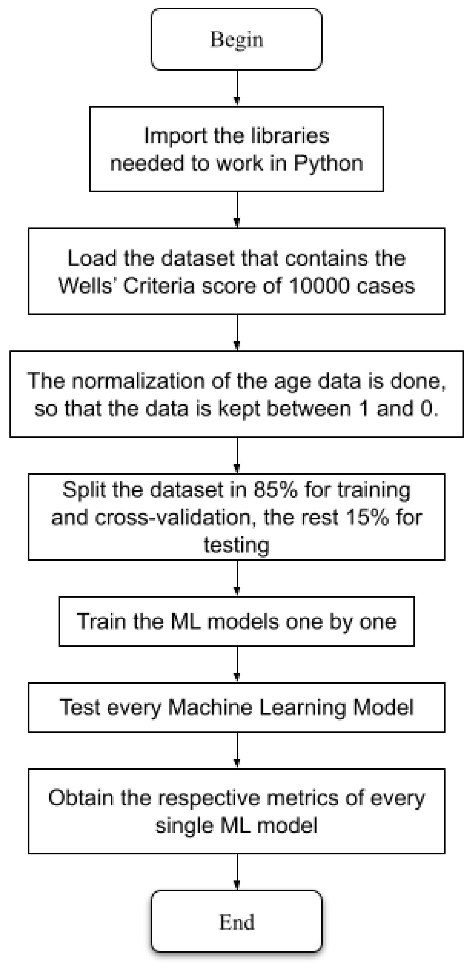
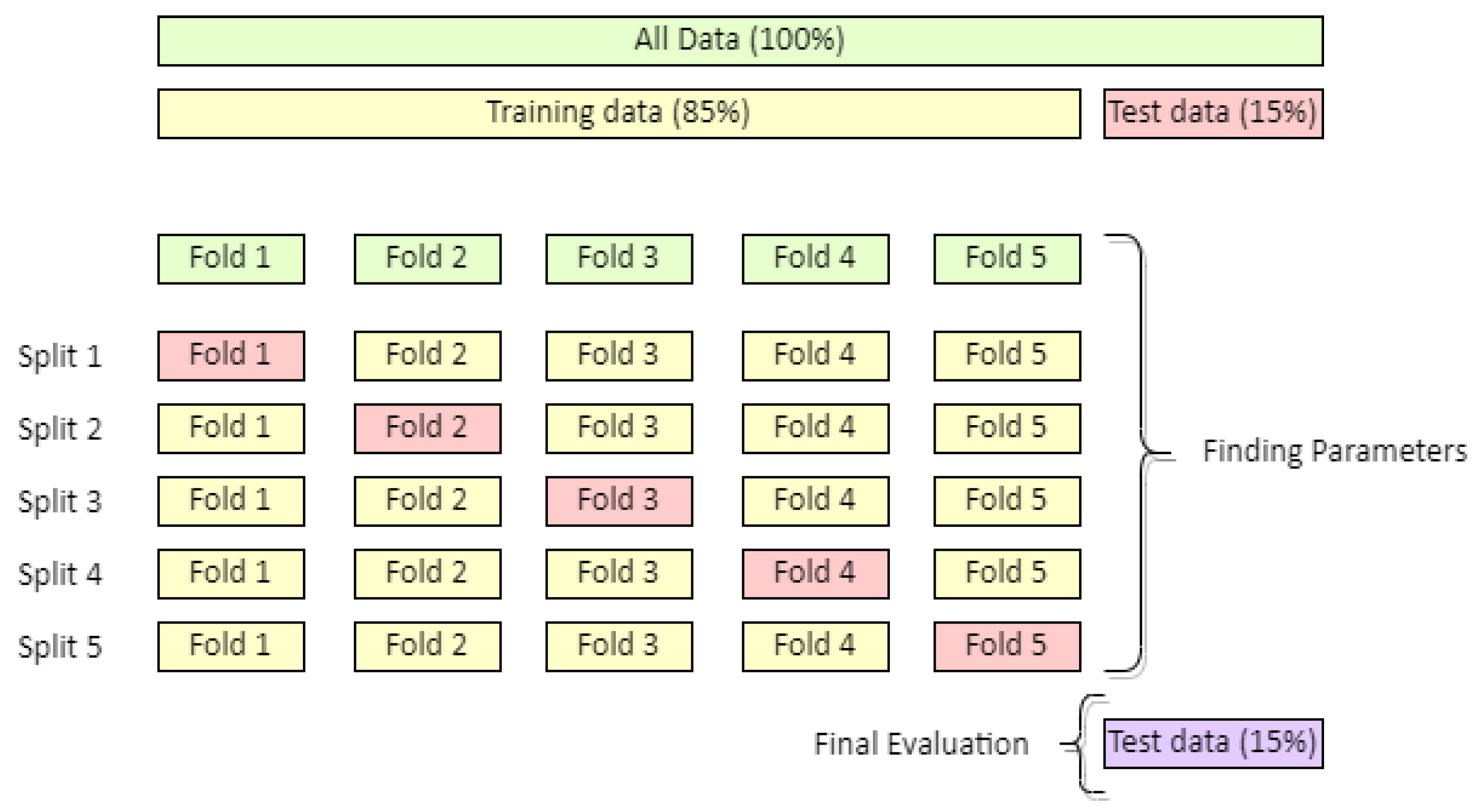
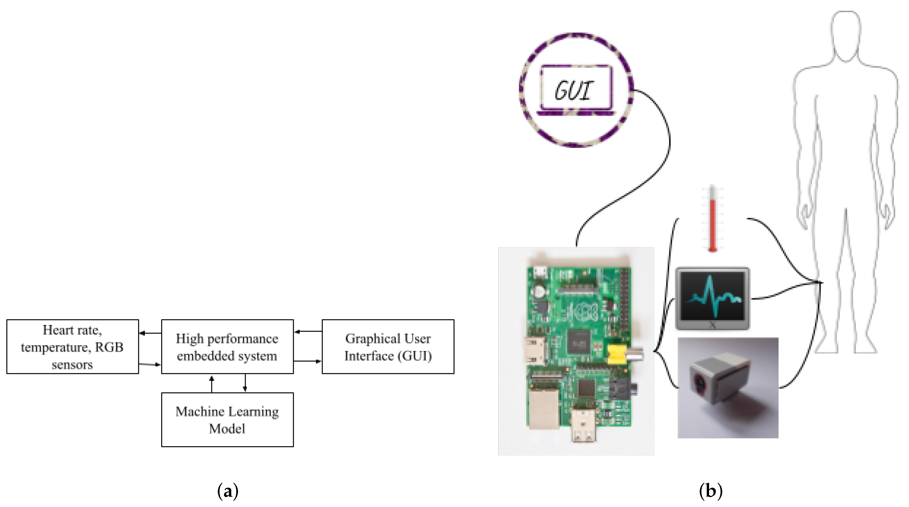
2. Materials and Methods

2.1. Machine Learning Algorithm Training

In this paper, we propose six ML algorithms to evaluate the occurrence of DVT in a patient: Decision Trees (DT), K-Nearest Neighbors (KNN), Support Vector Machine (SVM), Random Forest (RF), Multi-Layer Perceptron Neural Network (MLP-NN), and Extra Trees (ET). All of these ML models may be found in the Scikit Learn library [47,48]. The Scikit Learn library is built on top of NumPy, and it can be used for any kind of project. It has a lot of tools that can be used for both the pre- and post-processing of data. The flow chart for performing the ML algorithm training and testing is shown in Figure 1. First, it imports the appropriate libraries or toolboxes, such as Scikit Learn, Pandas, and Seaborn. Next, the features dataset is loaded, and the input data (features) and output data must be separated. Then, the dataset is randomly divided, with 85% used for training and cross-validation, and the remaining 15% used for testing. Next, the data are scaled between 0 and 1 to produce optimum results. Then, the ML algorithms is trained. Next, the ML model is scored, i.e., the confusion matrix and performance metrics are used to evaluate the ML models.

In this paper, a PC and RPi4 are used to train the ML models for DVT diagnosis, with the goal of testing their performance on both hardware and confirming that the RPi4’s scoring parameters and performance metrics are equally as trustworthy as those on a PC.

Table 1. RPi4 versus PC technical specifications comparison.

Hardware	Raspberry Pi 4	PC (Laptop)
Central Processing Unit (CPU)	Broadcom BCM2711 Quad Core 1.5 GHz	AMD Ryzen 7 4800H 2.9 GHz
Graphics Processing Unit (GPU)	Video Core VI 500 MHz	Nvidia GeForce GTX 1660ti
Random Access Memory (RAM)	4 GB DDR4	8 GB DDR4
Networking	WiFi, Ethernet, Bluetooth	WiFi, Ethernet, Bluetooth
Storage	32 GB SD-Card	512 GB SSD
Operating system	Raspbian	Windows 10
Operating Voltage	5 V	19.5 V
Energy consumption	3–7 Wh	200 Wh
Weight	46 g	2.37 Kg
Cost (USD)	$55.00	$1599.00

compares the RPi4’s primary technical specifications to those of a PC. While the hardware of the PC (laptop) obviously outperforms that of the RPi4, it is vital to prove experimentally that the results produced with the RPi4 are competitive to those obtained with a PC. Additionally, it is observed that the RPi4 is significantly less expensive than a PC, which would significantly lower manufacturing costs in a process of large-scale production of intelligent devices, for example, in the manufacture of hundreds or millions of smart instruments.

The dataset for this study was compiled from the following sources [10]. Since these data had been used previously, and only 59 real cases from a public hospital had been obtained, a data augmentation algorithm was devised. They are used to construct a dataset of 10,000 synthetic examples, which will be used for later training, validation, and testing as well as validation of the proposed ML models. The following process was used, as shown in Figure 1, and it will be detailed in depth in each stage below.

Data augmentation is a technique that is frequently used in machine learning to enhance the size of the dataset utilized in the learning process [10]. It entails producing new instances from the original data set while maintaining the data’s pattern. It is mostly used in medical contexts to augment the image collection for image-based diagnosis; see, for example [49,50,51,52]. In this paper, Algorithm (1) reported in [10] was used. It performs the data augmentation to generate each case that will comprise the set of synthetic data for training and validation of the proposed ML models. Therefore, the first task to be performed is to calculate the percentage of positive and negative cases that are present for each type of risk probability of the occurrence of DVT in addition to the percentage for which each of the factors of the Wells Score was observed in the real cases to which we had access. To calculate the percentage of suspected cases of DVT in each type of risk proposed by Wells, historical data was taken, where it is mentioned that of all the cases observed, 19% were diagnosed as DVT, while the remaining 81% had a different diagnosis. Furthermore, it is mentioned that in the cases detected as Low Risk, only 5% of the cases were diagnosed as positive for DVT, while 17% were diagnosed in Medium Risk, and 53% were diagnosed as High Risk.

The Wells Criteria, as shown in

Table 2. Wells criteria for predicting deep vein thrombosis (DVT), taken from [10,53,54,55].

Clinical Feature	Score
Lower extremity paralysis, paresis, or recent cast immobilization	1
Deep vein thrombosis has previously been observed	1
Active cancer (patients who are undergoing cancer therapy or who have been diagnosed with cancer within the last 6 months)	1
Pitting edema limited to the affected leg	1
Recently hospitalized for three or more days, or recently had major surgery Anesthesia is required for a total of 12 weeks	1
Tenderness in a specific area of the deep venous system’s distribution	1
Skinny veins on each sides (non-varicose)	1
The whole leg is swollen	1
Calf enlarged by at least 3 cm in comparison to the asymptomatic (ten centimeters below the tibial tuberosity)	1
Deep vein thrombosis is the most probable diagnosis; however, other possibilities exist.	−2
When a patient has symptoms in both legs, the leg with the most severe symptoms is utilized.

, are used to train the ML algorithms for the prediction of DVT, in which the trained models are expected to perform well in order to reach a high accuracy in the prediction of this condition.

2.2. Pre-Processing Data

Two criteria are taken into account that are not covered by the Wells rubric. The first is age, which is measured in numbers ranging from 1 to 9, each of which corresponds to one of the age groups listed in

Table 3. Age factor pre-processing, taken from [10].

Age (Years Old)	Life Stage	Numerical Value
85–120	Advanced old age	9
70–84	Intermediate old age	8
60–69	Initial old age	7
50–59	Mature adults	6
40–49	Average adults	5
21–39	Young adults	4
13–20	Youth	3
6–12	Middle childhood	2
0–5	Childhood	1

[10]. The second factor is gender, which is assigned a value of 0 to males and 1 to females. They are being offered as a way to help patients with suspected DVT better stratify their risk, just as it is managed in [23], so that the data collected may be pre-processed and ML can detect the illness without difficulty. Since the input data are binary, that is, they are regarded as 1 (for positive comorbidity) or 0 (for negative comorbidity), working with them in a computer system is simple, as most media handle binary values, with the age range being the main distinction, as weighted in Table 3.

The dataset is in Comma Separated Values (CSV) format in American Standard Code for Information Interchange (ASCII), so that it can be processed more easily in the Python environment, as well as in management so that it can be saved and extracted quickly. The data from the Excel file is fed into the software on the computer, using the Jupyter Notebook platform with Python, with each header referring to the DVT comorbidity in each of the columns. After that, using the Seaborn pairplot command, plots are generated between all of the data so that each of the values may be discriminated. It is required to normalize the values of 1–9 to values between 0 and 1 for good NN training.

Equation (1) is used to normalize the data in the age column so that this factor is not the most determinant or the one with the most weight within the ML model used. In this way, all the values of each clinical characteristic will be kept between 0 and 1 except for the age, which will be a floating value, and the others being integers.

$${\mathit{Norm}}_{\mathit{Age}}=\frac{Age-Mi{n}_{Age}}{Ma{x}_{Age}-Mi{n}_{Age}}$$

(1)

A data description is created to note specific properties of each column of information as well as the primary statistics of the values in the constructed dataset. We noted that the data is in a huge imbalance as a result of this, as it contains 7562 negative genuine cases and 2438 positive real cases.

The train test split function divides the dataset into 85% for training and 15% for validation, where the 11 input factors are considered clinical characteristics of the Wells criteria (cancer, immobilization, surgery, pain, leg swelling, ankle swelling, edema, superficial veins, and previously diagnosed DVT) and the factors of age and gender, respectively, and the output will result in the DVT diagnosis.

The K-fold cross-validation (with K = 5) is used to evaluate the performance of the ML models and perform a comparative analysis to select the model that best fits the DVT classification problem [56].

An early-stopping function has been constructed so that if there is no change of 0.01 in accuracy after 5 epochs, the model’s training is truncated and ended, so that the training does not take too long and the percentage of accuracy of the ML model employed during training does not vary much.

2.3. Hyperparameters of the ML Models

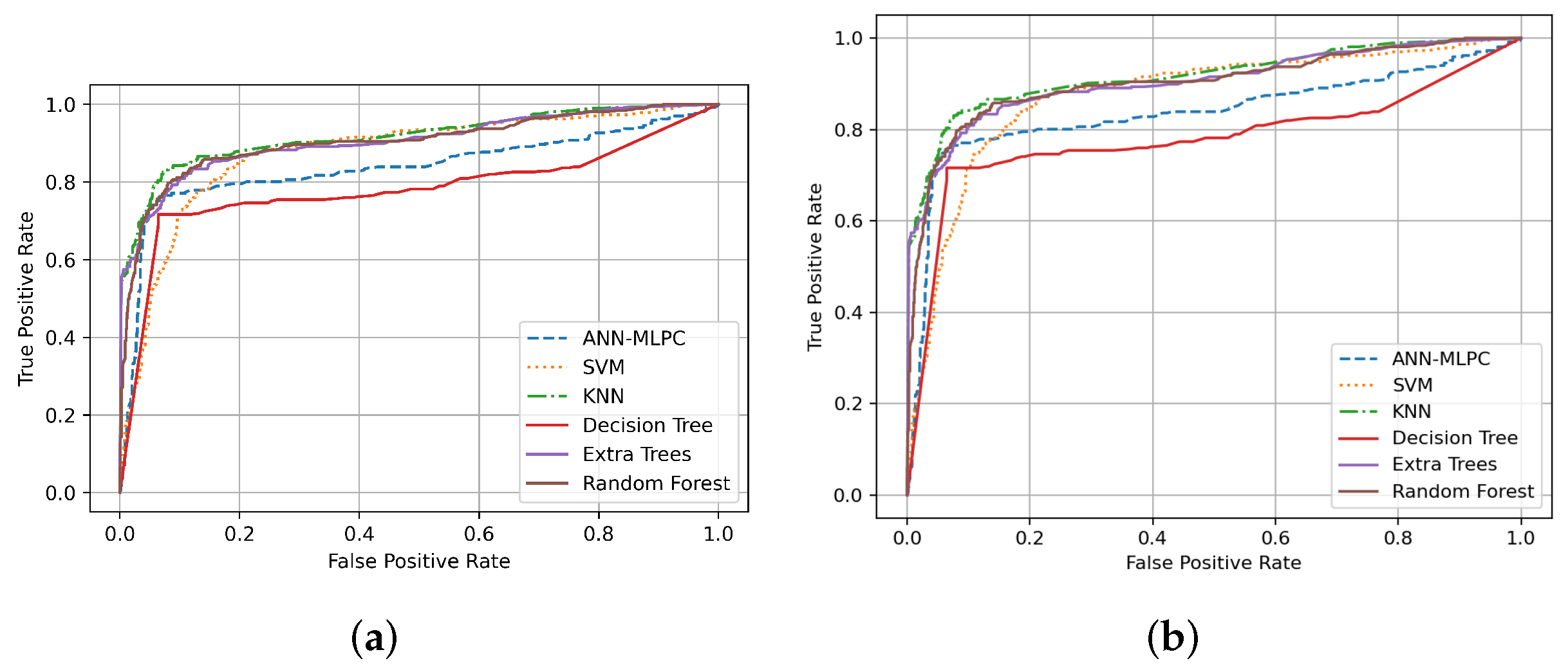
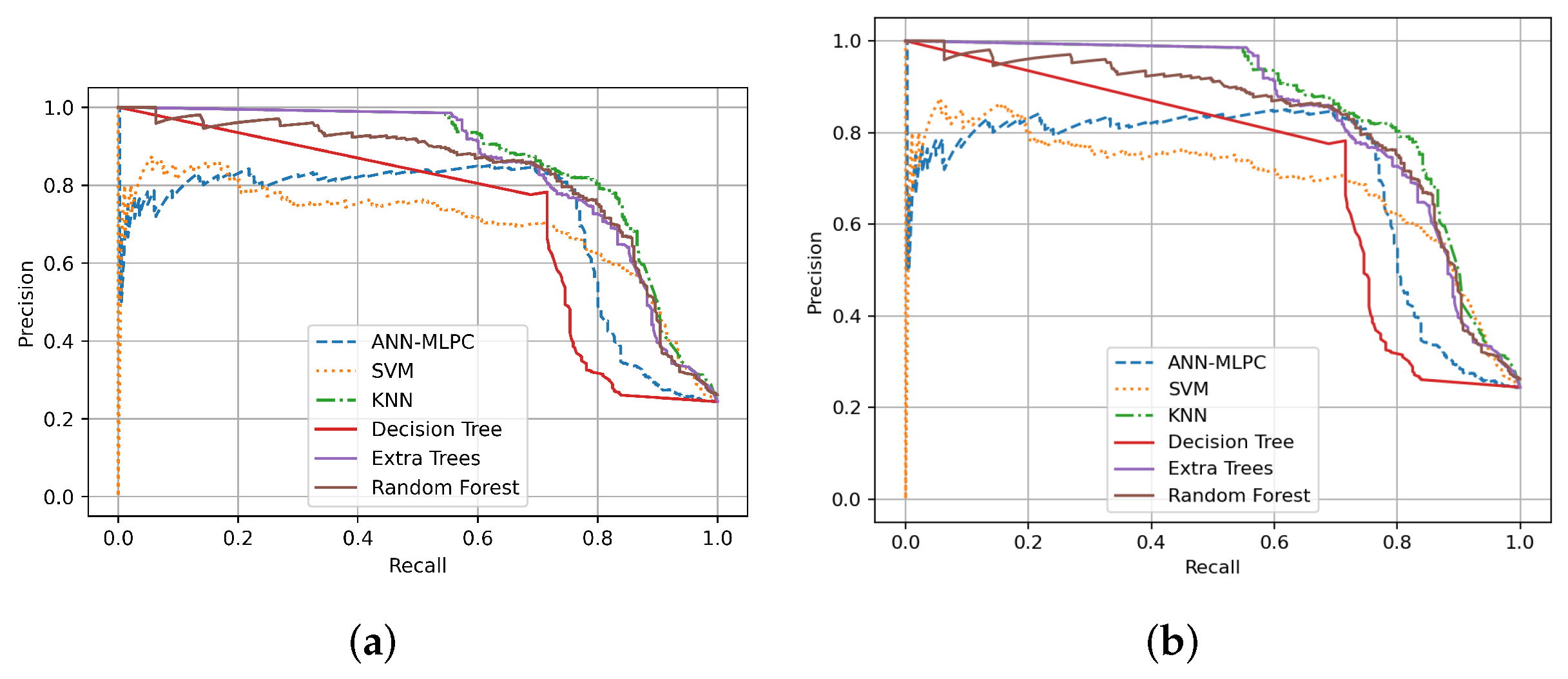
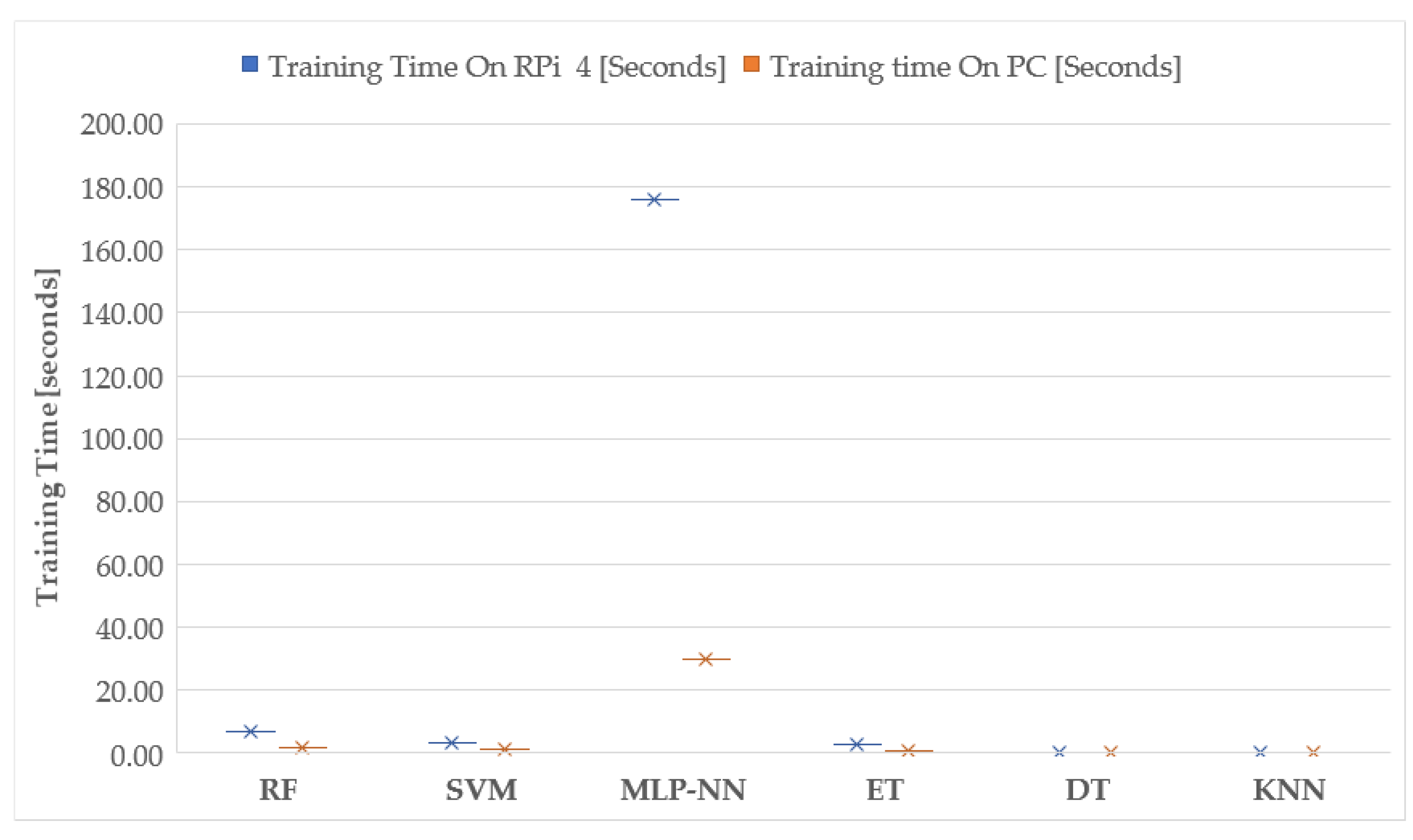
The use of an NN with table properties was first suggested during the creation of neural networks. It has an input layer with 11 predictors (cancer, immobility, surgery, pain, leg swelling, ankle swelling, edema, superficial veins, and previously diagnosed DVT). There is no magic formula for selecting the optimum number of hidden layers and neurons. However, some thumb rules are available for calculating the number of hidden layers and neurons. A rough approximation can be obtained by the geometric pyramid rule proposed by [57,58]. In this case, four hidden layers (32–64–32–16) were found for the best performance metrics, and an output layer with the DVT diagnosis is proposed, as shown in

Table 4. Proposed sequential model (NN) for DVT diagnosis.

Input Layer with 11 Predictors	Hidden Layer	Output Layer
Gender, age, cancer, surgery, immobilization, tenderness, leg swollen, calf swollen, edema, superficial veins, previous DVT	32–64–32–16	DVT diagnosis

. Since the computer is binary, it is suggested that the number of neurons per layer be multiples of $2^N$ for optimal processing time, where N is an integer, and the number of neurons in the first hidden layer should be greater than the number of inputs, being multiples of $2^N$, ascending in each hidden layer until a maximum of $2^N$ is reached and then descending with multiples of $2^N$ until the last hidden layer has a number of neurons slightly greater than the number of input neurons.

An input layer of 11 neurons, four hidden layers of 32, 64, 32, and 16 neurons, and an output layer representing the diagnostic result make up this ANN model. The input layer’s activation function is a relu function, while the hidden layers’ activation function is tanh, the learning rates of the classifier are defined as constant equal to 0.001, the max iteration number is 400, and with Adam as the optimizer.

The same ANN model is also trained on a Raspberry Pi 4 due to hardware limitations, and the hyperparameters of the classifiers are the same as the PC, only the results are slightly different and are discussed on Section 3. Furthermore, it is suggested that ML models be used in DVT diagnosis to compare each of the models, including SVM, KNN, DT, ET, and RF classifiers. The hyperparameters dealt with by the SVM classifier are as follows: a random state of 42, a C parameter of 1.0, a “linear” classifier kernel, a degree of 3, a gamma “scale”, and a random state of 3. The hyperparameters for the KNN classifier are as follows: the number of neighbors is set to 50, the weights are set to “distance”, and the algorithm is set to “ball tree”.

The Decision Tree classifier criteria used is “entropy”, the splitter is “random”, the minimum sample divisors is 2, the minimum leaf samples are given by 1, the maximum features are given by “auto”, the max features are 80, and there is a random state of 42.

The Extra Trees classifier is employed with a random state of 42 and many estimators of 200. The criterion utilized is “gini”, the minimum sample divisors is 2, the minimum leaf samples is 1, the maximum of features is “auto”, and the max features are given by 80.

Finally, the RF classifier has several estimators in 480, with “gini” as the criterion, 2 as the minimum sample divisors, 1 as the minimum number of leaf samples, “auto” as the maximum number of features, true Bootstrap, and 42 as the random state. All these hyperparameters are shown in the

Table 5. Hyperparameters of ML models.

Hyperparameter	SVM	KNN	Decision Tree	Extra Trees	Random Forest
C	1.0	N/A	N/A	N/A	N/A
Kernel	“linear”	N/A	N/A	N/A	N/A
Degree	3	N/A	N/A	N/A	N/A
Gamma	“scale”	N/A	N/A	N/A	N/A
Random State	42	42	42	42	42
N Neighbors	N/A	50	N/A	N/A	N/A
Weights	N/A	“Distance”	N/A	N/A	N/A
Algorithm	SVM	“Ball tree”	DT	ET	RF
Criterion	N/A	N/A	“Entropy”	“gini”	“gini”
Splitter	N/A	N/A	“Random”	N/A	N/A
Min Samples Split	N/A	N/A	2	2	2
Min Samples Leaf	N/A	N/A	1	1	1
Max Features	N/A	N/A	“auto”	“auto”	“auto”
Max Depth	N/A	N/A	80	80	N/A
N Estimators	N/A	N/A	N/A	200	480
Bootstrap	N/A	N/A	N/A	N/A	True

for every simulation in this paper.

To improve the performance of each classifier, the hyperparameters must be optimized. This can be accomplished using the GridSearchCV tool, which implements the standard estimator API. By “fitting” it to a dataset, all possible combinations of parameter values are evaluated, and only the best combination is kept. The chosen parameters maximize the score of the missing data unless an explicit score is given, in which case it is utilized instead of the default parameters for scoring [47,48]. The following classifiers have modified hyperparameters: the Random Forest and Extra Trees classifiers (Number of Estimators, Criterion, Max Features), the KNN classifier (Number of Neighbors, Weights, and Algorithm), the Decision Tree classifier (Criterion, Splitter, Max Features, and Max Depth), and the SVM classifier (C, Kernel, Degree (when using rbf, poly, and sigmoid)). They were distinct in each of them regarding the different possibilities dealt with. The optimization procedure is based on the “GridSearch” (GS) algorithm, which methodically calculates all possible combinations of hyperparameters. The main disadvantage is that it needs a significant amount of time and calculation [59].

The hardware used for the development of these experiments has the following specifications: AMD Ryzen 7 2.9 GHz CPU, 8 GB 3200 MHz DDR4 RAM, NVIDIA GeForce GTX 1660 Ti 6000 MB GPU, a Windows 10 operating system, and Python software with Anaconda 3. Similarly, a Raspberry Pi 4 SBC with the following specs: CPU 1.5 GHz Broadcom BXM2711, RAM 4GB 3200 MHz DDR4, Raspbian OS, and Python software with Thonny IDE was used to study the behavior of the ML in various contexts and system architectures. The following libraries utilized in this paper: Seaborn, which aids in statistical data visualization within Python; Pandas, which is a library to perform data analysis; NumPy, the platform’s data manipulation library; and Matplotlib, which is Python’s animated and interactive static visualization library. Scikit-Learn was used to create the ML models as well as custom neural networks.

3. Results

A two-class classification confusion matrix is developed to track the progress of the ML model trained, allowing the metrics to be validated and the process to be more dependable within the rubric by separating it into negative and positive DVT classifications, respectively.

Each of them is kept with the true diagnosis and the diagnosis predicted by the ML algorithm; the first is True Negative (TN), in which both the true diagnosis and the ML prediction are negative, and the second is False Negative (FN), in which the ML diagnosis is negative but the true diagnosis is positive for DVT. Another level of the confusion matrix is the False Positive (FP) criterion, which occurs when the algorithm diagnoses DVT as positive when the actual diagnosis is negative, and finally, the True Positive (TP) criterion, which occurs when the actual diagnosis is positive for the condition and the ML model prediction is positive, resulting in a True Positive (TP), as shown in

Table 6. Confusion matrix of two-class classification, taken from [10,60].

Predicted Diagnostic
True Diagnostic	Negative DVT	Positive DVT
Negative DVT	True Negative	False Positive
Positive DVT	False Negative	True Positive

.

For each ML model trained, the values of Accuracy, F1 Score, Precision, Recall, Specificity, and the area under the curve (AUC) are acquired and printed using sklearn metrics, the acquisition of Accuracy, Precision, Recall, and the ROC curve was accomplished in the case of the Multi-Layer Perceptron NN (MLP-NN), and the Accuracy (2), F1 score (3), Specificity (4), and Recall (5) values are calculated using the following equations taken from [24,61].

$$\mathit{Accuracy}=\frac{\mathit{True}\mathit{Positive}+\mathit{True}\mathit{Negative}}{\mathit{True}\mathit{Positive}+\mathit{False}\mathit{Positive}+\mathit{True}\mathit{Negative}+\mathit{False}\mathit{Positive}}$$

(2)

$$\mathit{F}\mathit{1}-\mathit{Score}=2·\frac{Precision·Recall}{Precision+Recall}$$

(3)

$$\mathit{Specificity}/\mathit{Precision}=\frac{\mathit{True}\mathit{Negative}}{\mathit{False}\mathit{Positive}+\mathit{True}\mathit{Negative}}$$

(4)

$$\mathit{Sensitivity}/\mathit{Recall}=\frac{\mathit{True}\mathit{Positive}}{\mathit{False}\mathit{Negative}+\mathit{True}\mathit{Positive}}$$

(5)

These actions are carried out for both PC and Raspberry Pi 4 metrics acquisition.

Table 7. Scoring parameters of the ML algorithms evaluated in this study using 15% of the separated data for testing.

	Machine Learning Algorithm on PC
Scoring Parameters	SVM	Decision Trees	Extra Trees	RF	MLP-NN	KNN
True Positive	265	262	268	274	274	292
True Negative	1017	1061	1060	1064	1067	1064
False Positive	117	73	74	70	67	70
False Negative	101	104	98	92	92	74
Accuracy	0.8546	0.8820	0.8853	0.8920	0.8940	0.9040
F1 Score	0.7085	0.7475	0.7570	0.7718	0.7751	0.8021
Specificity/Precision	0.6937	0.7820	0.7836	0.7965	0.8035	0.8066
Sensitivity/Recall	0.7240	0.7158	0.7322	0.7486	0.7486	0.7978
	Machine Learning Algorithm on RPi 4
Scoring Parameters	SVM	Decision Trees	Extra Trees	RF	MLP-NN	KNN
True Positive	265	262	268	274	274	292
True Negative	1017	1061	1060	1064	1067	1064
False Positive	117	73	74	70	67	70
False Negative	101	104	98	92	92	74
Accuracy	0.8546	0.8820	0.8853	0.8920	0.8940	0.9040
F1 Score	0.7085	0.7475	0.7570	0.7718	0.7751	0.8021
Specificity/Precision	0.6937	0.7820	0.7836	0.7965	0.8035	0.8066
Sensitivity/Recall	0.7240	0.7158	0.7322	0.7486	0.7486	0.7978

shows each of the scoring parameters gathered by each ML model (SVM, KNN, Decision Tree, Extra Trees, Random Forest), the ANN Multi-Layer Perceptron (MLP) model was also registered in the same way; each one includes the metrics (Accuracy, F1 Score, Precision/Specificity, and Recall/Sensitivity) as well as the values that each of the boxes of the two-class confusion matrix (True Positive, True Negative, False Positive and False Negative) gave, allowing you to see how these findings are obtained.

In terms of prediction model validation, there are two basic approaches utilized as selection criteria for a prediction model: (i) The hold-out model and (ii) the K-fold cross validation model. Both have the feature of utilizing a subset of the dataset for training and keeping a portion for validation. The K-fold cross-validation is a method that is utilized as a selection criterion for a prediction/classification model [56]. Essentially, it entails using a subset of the dataset to construct the model and leaving another portion of the dataset to validate it. The K-fold cross-validation procedure runs K times and averages the classification results for each interaction. As shown in Figure 2, it entails partitioning the dataset into k segments and selecting a different section to test the model K times. In contrast, the remaining K-1 elements are used to train the ML model [10,56]. The average values computed in the loop are the performance metrics supplied by K-fold cross-validation. This method is computationally expensive, but it does not waste a lot of data (unlike setting an arbitrary validation set), which is a big plus in applications such as inverse inference when the number of samples is small [47,48].

Table 8. Average results of K-fold cross-validation with K = 5 of the ML models trained on PC.

ML Model	K-Fold Cross-Validation with K = 5
	Accuracy	F1 Score	Specificity/Precision	Sensitivity/Recall	ROC-AUC
SVM	0.8468	0.6906	0.6804	0.7012	0.8589
Decision Trees	0.8677	0.7154	0.7528	0.6819	0.7562
Extra Trees	0.8710	0.7248	0.7552	0.6969	0.8831
RF	0.8744	0.7347	0.7576	0.7133	0.8830
MLP-NN	0.8632	0.7107	0.7347	0.6887	0.7924
KNN	0.8823	0.7586	0.7586	0.7586	0.8906

shows the average results of K-fold cross-validation corresponding to each ML model. In this study, we use K = 5 folds, and this assisted in validating all the scoring parameters of each ML model. The Accuracy, F1 score, Precision, Recall, and ROC-AUC were the metrics that could be achieved through this cross-validation; the ML model that had the best overall performance was the KNN, with the best scoring parameters, followed by RF in second place. Later, we found the Extra Trees model, in fourth place is MLP-NN, in fifth place are the Decision Trees, and last but not least is the SVM classifier.

Regarding the final evaluation (testing), Table 7 and

Table 9. Performance metrics of the six ML algorithms evaluated in this study using 15% of the separated data for testing.

	Performance Metrics on PC
Machine Learning Algorithm	ROC-AUC	PR-AUC	Cohen’s Kappa Coefficient	Hamming Loss	Matthew’s Correlation Coeficient
SVM	0.8104	0.6960	0.6118	0.1453	0.6120
Decision Trees	0.8257	0.6432	0.6707	0.1180	0.6718
Extra Trees	0.8334	0.8461	0.6821	0.1146	0.6828
Random Forest (RF)	0.8434	0.8283	0.7011	0.1080	0.7017
MLP-NN	0.8447	0.7102	0.7058	0.1060	0.7066
KNN	0.8680	0.8619	0.7388	0.0960	0.7388
	Performance Metrics on RPi 4
Machine Learning Algorithm	ROC-AUC	PR-AUC	Cohen’s Kappa Coefficient	Hamming Loss	Matthew’s Correlation Coeficient
SVM	0.8104	0.6954	0.6118	0.1453	0.6120
Decision Trees	0.8257	0.6432	0.6707	0.1180	0.6718
Extra Trees	0.8334	0.8461	0.6821	0.1146	0.6828
Random Forest (RF)	0.8434	0.8283	0.7011	0.1080	0.7017
MLP-NN	0.8447	0.7102	0.7058	0.1060	0.7066
KNN	0.8680	0.8619	0.7388	0.0960	0.7388

show the the outcomes of performance metrics when the ML models were tested with 15% of the dataset that was randomly split from the original dataset; i.e., this 15% of the data was kept separate from the dataset used for training; therefore, they had influence neither during training nor in cross-validation. As indicated in Table 7, the best ML model for this issue using PC is KNN, which has the greatest metrics. MLP-NN is second, Random Forest (RF) is third, Extra Trees is fourth, Decision Trees is fifth, and lastly, we have the SVM model that is sixth. Within these rubrics, the accuracy values of the ML models are very good, ranging from 85.4% (SVM) to 90.4% (KNN), as well as the specificity of the model, which is somewhat deplorable in the case of the SVM, being the lowest with 69.37 %, but the others far exceed it, with the KNN classifier reaching 80.66%. It also possessed a superior comparative response to the angiologist physician metrics of 73.82% in accuracy and a specificity of 71.43% [10], proving to be a better technique to detect DVT.

Despite its restricted technology, the Raspberry Pi 4 achieves good results, attaining the same metrics as the PC with no differences, demonstrating the strength of the SystemOnChip (SoC), which is ideal for moving this type of diagnosis to smart devices. Despite the embedded system’s limited computational capability, excellent metrics for a portable intelligent system are attained, outperforming the Wells technique in a typical approach.

Receiver Operating Characteristic (ROC) curves can be generated using the aforementioned data, which indicate how well the model can distinguish between two objects. They are key metrics for assessing an ML model’s performance. Furthermore, they are employed in binary classification issues, i.e., problems with two distinct output classes. The connection between the model’s True Positive Rate (TPR) and False Positive Rate (FPR) is depicted by the ROC curve.

Both the ROC curve on PC and the ROC curve on Raspberry Pi 4 have a similar response; the KNN model has a larger area under the curve, making it more visually appealing, which is complemented by the scoring metrics mentioned in Table 7, which is followed by the Random Forest (RF) classifier, as shown in Figure 3.

Similarly, it is possible to obtain PR curves (Precision–Recall curves), which are a useful measure for observing prediction success when classes are highly disequilibrated or unbalanced. In information retrieval, precision is a measure of the relevance of the results, whereas recall is a measure of the number of truly relevant results that are returned. The PR curve depicts the trade-off between Precision and Recall at various levels. A high area under the curve indicates both High Recall and High Precision, with High Precision corresponding to a low False Positive Rate and high Recall corresponding to a low False Negative Rate. High scores in both cases show that the classifier is delivering accurate (High Precision) results as well as the bulk of positive outcomes (High Recall).

Figure 4 shows that the PR curves of the Raspberry Pi 4 and PC are similar; the KNN classifier has a better PR curve over all classifiers in both cases, having a larger area under the curve covered within the graph, making it one of the best classifiers, followed by the Extra Trees classifier.

The next step is to obtain the performance metrics to evaluate the ML models; we rely on the metrics of the Scikit learn library. The performance metrics are the Area Under the Curve (AUC) using the trapezoidal method, the Cohen’s Kappa coefficient, Hamming Loss, and Matthew’s correlation coefficient, all of which are achieved on a PC and a Raspberry Pi 4 correspondingly, which are listed in Table 9.

According to Table 9, the KNN classifier is the best binary ML classifier for PC in terms of performance metrics, followed by Random Forest (RF) in second, the Extra Trees classifier in third, MLP-NN model in fourth, Decision Trees classifier in fifth, and last but not least, the SVM classifier. The system’s measurements show an AUC ranging from 81.04% with the SVM model to 86.80% with the KNN classifier. The Hamming Loss is another metric that goes from SVM at 14.53% to the best with a lower percentage, the KNN model at 9.60%.

For its part, the Raspberry Pi 4 achieved good results, which are identical in theory to those acquired by the PC, when all of the parameters involved in each of the classifiers, during training, and determining the performance metrics and score were taken into account.

The average time of each of the proposed classifiers to be used within this problem was obtained both on PC and Raspberry Pi 4. Figure 5 shows the average time of ten training runs of each model with their respective characteristics, both on the computer and on the SoC, to analyze the cost–benefit of each of the proposed classifiers to be used within this problem. Due to factors of processing power operations, it turns out to be faster than the Raspberry Pi 4, with the Decision Trees model being the fastest, followed closely by the KNN, and further behind the Extra Trees, all with a training time of less than a second, then the SVM, before reaching 2 s, the RF classifier, and finally, the MLP-NN being the slowest of all with a time greater than 30 s. The training on the Raspberry Pi 4 takes two to five times longer due to the embedded system’s processing limitations, with times of 0.02 s in Decision Trees, 0.1 s in KNN models, 2.81 s in Extra Trees, 3.12 s in SVM, 6.89 s in RF models, and finally 175.85 s in RF models.

Usage Scenario

These ML models could be implemented on an embedded system such as the Raspberry Pi 4 (RPi4) to develop a DVT diagnostic smart system. This could be integrated with a color sensor (RGB), heart rate (BPM), and temperature (°C), as well as a user interface (GUI) that may include some questions according to the Wells criteria. Furthermore, the physician can acquire the raw Wells criteria for each patient to be diagnosed with this proposed system. The smart system will have a trained ML model into which the selected patient’s data will be entered, and it will provide a diagnosis prediction for the patient’s condition. The prospective apparatus proposed by this research can be shown in Figure 6. As discussed before and shown in Table 1, the RPi4 is less expensive than a PC, which would result in significant cost savings associated with the large-scale production of intelligent devices, such as the manufacture of hundreds or millions of smart instruments.

4. Conclusions

Multiple ML classifiers were assessed for the prediction of DVT in the lower limbs according to Wells criteria. They were subjected to different score and performance metrics to assist with identifying the dependability of each one. The results of each of the created models were subjected to cross-validation. The experimental results show that the KNN model is the best in terms of performance and score metrics (higher accuracy (90.40%), higher specificity (80.66%), ROC-AUC (86.80%), and PR-AUC (86.16%)), but it is second in terms of execution time (0.01904 s) followed by the MLP-NN model, which is the slowest in terms of execution time (30.08 s), but gives us the second best accuracy (89.40%). The KNN classifier, on the other hand, among the models trained on the Raspberry Pi 4, has the same score and performance metrics as on the PC; the main difference is in the execution time, as it takes 0. 0951 s to train the model, making it the second in this category; however, in real terms, it is possible to wait a little longer for a portable result, and in second place is the MLP-NN classifier, with an execution time of 175.8485 s, making it the slowest. The accuracy of all trained models on PC and Raspberry Pi 4 is greater than 85%, while the AUC values are between 81 and 86%. In conclusion, as compared to traditional methods, the best ML classifiers were effective at predicting DVT diagnosis in a timely and efficient manner.

References

1. Yang, M.; Tan, T. Formation of Thrombosis and Its Potential Diagnosis and Treatment with Optoacoustic Technology. In Proceedings of the Third International Conference on Medical and Health Informatics 2019 (ICMHI 2019), Xiamen, China, 17–19 May 2019; pp. 1–5. [Google Scholar] [CrossRef]
2. Liu, K.; Chen, J.; Zhang, K.; Wang, S.; Li, X. A Diagnostic Prediction Model of Acute Symptomatic Portal Vein Thrombosis. Ann. Vasc. Surg. 2019, 61, 394–399. [Google Scholar] [CrossRef] [PubMed]
3. Kim, D.; Byyny, R.; Rice, C.; Faragher, J.; Nordenholz, K.; Haukoos, J.; Liao, M.; Kendall, J. Test Characteristics of Emergency Physician-Performed Limited Compression Ultrasound for Lower-Extremity Deep Vein Thrombosis. J. Emerg. Med. 2016, 51, 684–690. [Google Scholar] [CrossRef] [PubMed]
4. Moore, R.D.; Pryce, W.I.J.; Todd, J.M. The use of the ultrasonic Doppler test in the detection of deep vein thrombosis. Phys. Med. Biol. 1973, 18, 142–143. [Google Scholar] [CrossRef]
5. Penco, S.; Grossi, E.; Cheng, S.; Intraligi, M.; Maurelli, G.; Patrosso, M.; Marocchi, A.; Buscema, M. Assessment of Genetic Polymorphism Role in Venous Thrombosis Through Artificial Neural Networks. Ann. Hum. Genet. 2005, 69, 693–706. [Google Scholar] [CrossRef]
6. Wang, X.; Yang, Y.Q.; Liu, S.H.; Hong, X.Y.; Sun, X.F.; Shi, J.H. Comparing different venous thromboembolism risk assessment machine learning models in Chinese patients. J. Eval. Clin. Pract. 2019, 26, 26–34. [Google Scholar] [CrossRef]
7. Luo, L.; Kou, R.; Feng, Y.; Xiang, J.; Zhu, W. Cost-Effective Machine Learning Based Clinical Pre-Test Probability Strategy for DVT Diagnosis in Neurological Intensive Care Unit. Clin. Appl. Thromb. 2021, 27, 10760296211008650. [Google Scholar] [CrossRef]
8. Ferroni, P.; Zanzotto, F.M.; Scarpato, N.; Riondino, S.; Guadagni, F.; Roselli, M. Validation of a Machine Learning Approach for Venous Thromboembolism Risk Prediction in Oncology. Dis. Markers 2017, 2017, 8781379. [Google Scholar] [CrossRef] [Green Version]
9. Riondino, S.; Ferroni, P.; Zanzotto, F.M.; Roselli, M.; Guadagni, F. Predicting VTE in cancer patients: Candidate biomarkers and risk assessment models. Cancers 2019, 11, 95. [Google Scholar] [CrossRef] [Green Version]
10. Fong-Mata, M.; Garcia-Guerrero, E.; Mejia-Medina, D.; Lopez-Bonilla, O.; Villarreal-Gomez, L.; Zamora-Arellano, F.; Lopez-Mancilla, D.; Inzunza-Gonzalez, E. An Artificial Neural Network Approach and a Data Augmentation Algorithm to Systematize the Diagnosis of Deep-Vein Thrombosis by Using Wells’ Criteria. Electronics 2020, 9, 1810. [Google Scholar] [CrossRef]
11. Segal, J.B.; Eng, J.; Tamariz, L.J.; Bass, E.B. Review of the Evidence on Diagnosis of Deep Venous Thrombosis and Pulmonary Embolism. Ann. Fam. Med. 2007, 5, 63. [Google Scholar] [CrossRef] [Green Version]
12. Smyrnakis, E.; Symintiridou, D.; Andreou, M.; Dandoulakis, M.; Theodoropoulos, E.; Kokkali, S.; Manolaki, C.; Papageorgiou, D.I.; Birtsou, C.; Paganas, A.; et al. Primary care professionals’ experiences during the first wave of the COVID-19 pandemic in Greece: A qualitative study. BMC Fam. Pract. 2021, 22, 174. [Google Scholar] [CrossRef]
13. da Silva, L.G.R.; da Silva Pinto, A.W.; de Queiroz, W.E.; Coelho, C.C.; Blatt, C.R.; Oliveira, M.G.; de Lima Pimentel, A.C.; Elseviers, M.; Baldoni, A.O. Deprescribing clonazepam in primary care older patients: A feasibility study. Int. J. Clin. Pharm. 2022. [Google Scholar] [CrossRef] [PubMed]
14. Győrffy, Z.; Békási, S.; Döbrössy, B.; Bognár, V.K.; Radó, N.; Morva, E.; Zsigri, S.; Tari, P.; Girasek, E. Exploratory attitude survey of homeless persons regarding telecare services in shelters providing mid- and long-term accommodation: The importance of trust. PLoS ONE 2022, 17, e0261145. [Google Scholar] [CrossRef] [PubMed]
15. Wells, P. Predictive analytics by deep machine learning: A call for next-gen tools to improve health care. Res. Pract. Thromb. Haemost. 2020, 4, 181–182. [Google Scholar] [CrossRef] [PubMed]
16. Yokomichi, A.; Rodrigues, V.; Moroz, A.; Bertanha, M.; Ribeiro, S.; Defune, E.; Moraes, M. Detection of Factor VIII and D-dimer biomarkers for venous thromboembolism diagnosis using electrochemistry immunosensor. Talanta 2020, 219, 121241. [Google Scholar] [CrossRef]
17. Kacmaz, S.; Ercelebi, E.; Zengin, S.; Cindoruk, S. The Use of Infrared Thermal Imaging in the Diagnosis of Deep Vein Thrombosis. Infrared Phys. Technol. 2017, 86, 120–129. [Google Scholar] [CrossRef]
18. Tanno, R.; Makropoulos, A.; Arslan, S.; Oktay, O.; Mischkewitz, S.; Noor, F.; Oppenheimer, J.; Mandegaran, R.; Kainz, B.; Heinrich, M. AutoDVT: Joint Real-Time Classification for Vein Compressibility Analysis in Deep Vein Thrombosis Ultrasound Diagnostics. In Proceedings of the 21st International Conference, Granada, Spain, 16–20 September 2018; Part II. pp. 905–912. [Google Scholar] [CrossRef]
19. Kainz, B.; Heinrich, M.P.; Makropoulos, A.; Oppenheimer, J.; Mandegaran, R.; Sankar, S.; Deane, C.; Mischkewitz, S.; Al-Noor, F.; Rawdin, A.C.; et al. Non-invasive diagnosis of deep vein thrombosis from ultrasound imaging with machine learning. NPJ Digit. Med. 2021, 4, 137. [Google Scholar] [CrossRef]
20. Lewiss, R.E.; Kaban, N.L.; Turandot, S. Point-of-Care Ultrasound for a Deep Venous Thrombosis. Glob. Heart 2013, 8, 329–333. [Google Scholar] [CrossRef] [Green Version]
21. Ly-Pen, D.; Penedo-Alonso, R.; Sánchez-Pérez, M. Comparison of the Accuracy of Emergency Department–Performed Point-of-Care Ultrasound in the Diagnosis of Lower-Extremity Deep Vein Thrombosis. J. Emerg. Med. 2018, 55, 716–717. [Google Scholar] [CrossRef]
22. Huang, C.; Tian, J.; Yuan, C.; Zeng, P.; He, X.; Chen, H.; Huang, Y.; Huang, B. Fully Automated Segmentation of Lower Extremity Deep Vein Thrombosis Using Convolutional Neural Network. BioMed Res. Int. 2019, 2019, 3401683. [Google Scholar] [CrossRef] [Green Version]
23. Willan, J.; Katz, H.; Keeling, D. The use of artificial neural network analysis can improve the risk-stratification of patients presenting with suspected deep vein thrombosis. Br. J. Haematol. 2019, 185, 289–296. [Google Scholar] [CrossRef] [PubMed]
24. Fong-Mata, M.B.; Inzunza-Gonzalez, E.; Garcia-Guerrero, E.; Mejia-Medina, D.; Morales Contreras, O.; Gomez-Roa, A. Trombosis venosa profunda en extremidades inferiores: Revisión de las técnicas de diagnóstico actuales y su simbiosis con el aprendizaje automático para un diagnóstico oportuno. Rev. Cienc. Tecnol. 2020, 3, 23–34. [Google Scholar] [CrossRef]
25. Litjens, G.; Kooi, T.; Ehteshami Bejnordi, B.; Adiyoso Setio, A.A.; Ciompi, F.; Ghafoorian, M.; Van Der Laak, J.A.W.M.; Van Ginneken, B.; Sánchez, C.I. A survey on deep learning in medical image analysis. Med. Image Anal. 2017, 42, 60–88. [Google Scholar] [CrossRef] [PubMed] [Green Version]
26. Agharezaei, L.; Agharezaei, Z.; Nemati, A.; Bahaadinbeigy, K.; Keynia, F.; Baneshi, M.; Iranpour, A.; Agharezaei, M. The Prediction of the Risk Level of Pulmonary Embolism and Deep Vein Thrombosis through Artificial Neural Network. Acta Inform. Med. 2016, 24, 354. [Google Scholar] [CrossRef] [PubMed] [Green Version]
27. Sukperm, A.; Rojnuckarin, P.; Akkawat, B.; Sa-Ing, V. Automatic Diagnosis of Venous Thromboembolism Risk based on Machine Learning. In Proceedings of the 2021 IEEE International IOT, Electronics and Mechatronics Conference (IEMTRONICS), Toronto, ON, Canada, 21–24 April 2021; pp. 1–4. [Google Scholar] [CrossRef]
28. Liu, H.; Yuan, H.; Wang, Y.; Huang, W.; Xue, H.; Zhang, X. Prediction of venous thromboembolism with machine learning techniques in young-middle-aged inpatients. Sci. Rep. 2021, 11, 12868. [Google Scholar] [CrossRef]
29. Ferroni, P.; Zanzotto, F.M.; Scarpato, N.; Riondino, S.; Nanni, U.; Roselli, M.; Guadagni, F. Risk Assessment for Venous Thromboembolism in Chemotherapy-Treated Ambulatory Cancer Patients: A Machine Learning Approach. Med. Decis. Mak. 2016, 37, 234–242. [Google Scholar] [CrossRef]
30. Egwuche, O.S.; Ganiyu, M.; Ibiyomi, M.A. A survey of mobile edge computing in developing countries: Challenges and prospects. J. Phys. Conf. Ser. 2021, 2034, 012004. [Google Scholar] [CrossRef]
31. Liu, L.; Chen, L.; Xu, S.; Xu, Y.; Shi, C. Design and implementation of intelligent monitoring terminal for distribution room based on edge computing. Energy Rep. 2021, 7, 1131–1138. [Google Scholar] [CrossRef]
32. Andrawes, A.; Nordin, R.; Albataineh, Z.; Alsharif, M.H. Sustainable delay minimization strategy for mobile edge computing offloading under different network scenarios. Sustainability 2021, 13, 12112. [Google Scholar] [CrossRef]
33. Teng, Y.; Cui, J.; Jiang, W. Research on application of edge computing in real-time environmental monitoring system. J. Phys. Conf. Ser. 2021, 2010, 012157. [Google Scholar] [CrossRef]
34. Alessio, K.; Tischer, B.; Voss, M.; Teixeira, I.; Brendler, B.; Duarte, F.; Helfer, G.; Costa, A.; Barin, J. Open source, low-cost device for thermometric titration with non-contact temperature measurement. Talanta 2020, 216, 120975. [Google Scholar] [CrossRef] [PubMed]
35. Nykvist, C.; Larsson, M.; Sodhro, A.; Gurtov, A. A lightweight portable intrusion detection communication system for auditing applications. Int. J. Commun. Syst. 2020, 33, e4327. [Google Scholar] [CrossRef]
36. Zamora-Arellano, F.; López-Bonilla, O.R.; García-Guerrero, E.E.; Olguín-Tiznado, J.E.; Inzunza-González, E.; López-Mancilla, D.; Tlelo-Cuautle, E. Development of a Portable, Reliable and Low-Cost Electrical Impedance Tomography System Using an Embedded System. Electronics 2021, 10, 15. [Google Scholar] [CrossRef]
37. Gautam, A.; Kumar, A.; Kinjalk, K.; Thangaraj, J.; Priye, V. A Low Cost FBG Based Online Weight Monitoring System. IEEE Sens. J. 2020, 20, 4207–4214. [Google Scholar] [CrossRef]
38. Nirmala, M.; Malarvizhi, K. Internet of things based solar powered truck. Test Eng. Manag. 2020, 83, 9358–9365. [Google Scholar]
39. Aguirre-Castro, O.; Inzunza-González, E.; García-Guerrero, E.; Tlelo-Cuautle, E.; López-Bonilla, O.; Olguín-Tiznado, J.; Cárdenas-Valdez, J. Design and Construction of an ROV for Underwater Exploration. Sensors 2019, 19, 5387. [Google Scholar] [CrossRef] [Green Version]
40. Dhatri, M.P.; Shivram, R. Development of a Functional Testing System for Test Automation and Statistical Analysis of the behavior of health care device used to treat Deep Vein Thrombosis. In Proceedings of the 2018 3rd IEEE International Conference on Recent Trends in Electronics, Information & Communication Technology (RTEICT), Bangalore, India, 18–19 May 2018; pp. 1715–1719. [Google Scholar] [CrossRef]
41. Cerrada, M.; Trujillo, L.; Hernández, D.E.; Correa Zevallos, H.A.; Macancela, J.C.; Cabrera, D.; Vinicio Sánchez, R. AutoML for Feature Selection and Model Tuning Applied to Fault Severity Diagnosis in Spur Gearboxes. Math. Comput. Appl. 2022, 27, 6. [Google Scholar] [CrossRef]
42. Enríquez Zárate, J.; Gómez López, M.d.l.A.; Carmona Troyo, J.A.; Trujillo, L. Analysis and Detection of Erosion in Wind Turbine Blades. Math. Comput. Appl. 2022, 27, 5. [Google Scholar] [CrossRef]
43. Esqueda-Elizondo, J.J.; Juarez-Ramirez, R.; Lopez-Bonilla, O.R.; Garcia-Guerrero, E.E.; Galindo-Aldana, G.M.; Jimenez-Beristain, L.; Serrano-Trujillo, A.; Tlelo-Cuautle, E.; Inzunza-Gonzalez, E. Attention Measurement of an Autism Spectrum Disorder User Using EEG Signals: A Case Study. Math. Comput. Appl. 2022, 27, 21. [Google Scholar] [CrossRef]
44. Nwosisi, C.; Sung-Hyuk, C.; Yoo, J.A.; Tappert, C.C.; Lipsitz, E. Constructing Binary Decision Trees for Predicting Deep Venous Thrombosis. In Proceedings of the 2010 2nd International Conference on Software Technology and Engineering, San Juan, PR, USA, 3–5 October 2010; Volume 1, pp. V1-121–V1-124. [Google Scholar] [CrossRef]
45. Nafee, T.; Gibson, C.M.; Travis, R.; Yee, M.K.; Kerneis, M.; Chi, G.; AlKhalfan, F.; Hernandez, A.F.; Hull, R.D.; Cohen, A.T.; et al. Machine learning to predict venous thrombosis in acutely ill medical patients. Res. Pract. Thromb. Haemost. 2020, 4, 230–237. [Google Scholar] [CrossRef] [Green Version]
46. Ryan, L.; Mataraso, S.; Siefkas, A.; Pellegrini, E.; Barnes, G.; Green-Saxena, A.; Hoffman, J.; Calvert, J.; Das, R. A Machine Learning Approach to Predict Deep Venous Thrombosis Among Hospitalized Patients. Clin. Appl. Thromb. 2021, 27, 1076029621991185. [Google Scholar] [CrossRef] [PubMed]
47. Pedregosa, F.; Varoquaux, G.; Gramfort, A.; Michel, V.; Thirion, B.; Grisel, O.; Blondel, M.; Prettenhofer, P.; Weiss, R.; Dubourg, V.; et al. Scikit-learn: Machine Learning in Python. J. Mach. Learn. Res. 2011, 12, 2825–2830. [Google Scholar]
48. Buitinck, L.; Louppe, G.; Blondel, M.; Pedregosa, F.; Mueller, A.; Grisel, O.; Niculae, V.; Prettenhofer, P.; Gramfort, A.; Grobler, J.; et al. API design for machine learning software: Experiences from the scikit-learn project. In Proceedings of the European Conference on Machine Learning and Principles and Practice of Knowledge Discovery in Databases (ECMLPKDD 2013), Prague, Czech Republic, 23–27 September 2013; pp. 108–122. [Google Scholar]
49. Liu, Z.; Cao, Y.; Li, Y.; Xiao, X.; Qiu, Q.; Yang, M.; Zhao, Y.; Cui, L. Automatic diagnosis of fungal keratitis using data augmentation and image fusion with deep convolutional neural network. Comput. Methods Programs Biomed. 2020, 187, 105019. [Google Scholar] [CrossRef] [PubMed]
50. Zuluaga-Gomez, J.; Al Masry, Z.; Benaggoune, K.; Meraghni, S.; Zerhouni, N. A CNN-based methodology for breast cancer diagnosis using thermal images. Comput. Methods Biomech. Biomed. Eng. Imaging Vis. 2020, 9, 131–145. [Google Scholar] [CrossRef]
51. de Souza, L.A.; Passos, L.A.; Mendel, R.; Ebigbo, A.; Probst, A.; Messmann, H.; Palm, C.; Papa, J.P. Assisting Barrett’s esophagus identification using endoscopic data augmentation based on Generative Adversarial Networks. Comput. Biol. Med. 2020, 126, 104029. [Google Scholar] [CrossRef] [PubMed]
52. Gao, Z.; Li, J.; Guo, J.; Chen, Y.; Yi, Z.; Zhong, J. Diagnosis of Diabetic Retinopathy Using Deep Neural Networks. IEEE Access 2019, 7, 3360–3370. [Google Scholar] [CrossRef]
53. Wells, P.S.; Anderson, D.R.; Bormanis, J.; Guy, F.; Mitchell, M.; Gray, L.; Clement, C.; Robinson, K.S.; Lewandowski, B. Value of assessment of pretest probability of deep-vein thrombosis in clinical management. Lancet 1997, 350, 1795–1798. [Google Scholar] [CrossRef]
54. Wells, P.S.; Owen, C.; Doucette, S.; Fergusson, D.; Tran, H. Does this patient have deep vein thrombosis? JAMA 2006, 295, 199–207. [Google Scholar] [CrossRef]
55. Modi, S.; Deisler, R.; Gozel, K.; Reicks, P.; Irwin, E.; Brunsvold, M.; Banton, K.; Beilman, G.J. Wells criteria for DVT is a reliable clinical tool to assess the risk of deep venous thrombosis in trauma patients. World J. Emerg. Surg. 2016, 11, 24. [Google Scholar] [CrossRef] [Green Version]
56. Jung, Y. Multiple predicting K-fold cross-validation for model selection. J. Nonparametr. Stat. 2018, 30, 197–215. [Google Scholar] [CrossRef]
57. Pano-Azucena, A.; Tlelo-Cuautle, E.; Tan, S.D.; Ovilla-Martinez, B.; De la Fraga, L. FPGA-Based Implementation of a Multilayer Perceptron Suitable for Chaotic Time Series Prediction. Technologies 2018, 6, 90. [Google Scholar] [CrossRef] [Green Version]
58. Kaufmann, M. Practical Neural Networks Recipes in C++; Elsevier: Boston, MA, USA, 1993; p. 493. [Google Scholar] [CrossRef]
59. Vávra, J.; Hromada, M.; Lukáš, L.; Dworzecki, J. Adaptive anomaly detection system based on machine learning algorithms in an industrial control environment. Int. J. Crit. Infrastruct. Prot. 2021, 34, 100446. [Google Scholar] [CrossRef]
60. Sadrawi, M.; Sun, W.Z.; Ma, M.M.; Yeh, Y.T.; Abbod, M.; Shieh, J.S. Ensemble genetic fuzzy neuro model applied for the emergency medical service via unbalanced data evaluation. Symmetry 2018, 10, 71. [Google Scholar] [CrossRef] [Green Version]
61. Sokolova, M.; Japkowicz, N.; Szpakowicz, S. Beyond Accuracy, F-Score and ROC: A Family of Discriminant Measures for Performance Evaluation. In Proceedings of the 19th Australian Joint Conference on Artificial Intelligence, Hobart, Australia, 4–8 December 2006; pp. 1015–1021. [Google Scholar]
Figure 1. Proposed methodology for early diagnosis of DVT.
Mca 27 00024 g001
Figure 2. Scheme of the K-fold cross-validation for the proposed ML models, inspired from [47,48].
Mca 27 00024 g002
Figure 3. ROC curves. (a) ROC curve on PC, and (b) ROC curve on Raspberry Pi 4.
Mca 27 00024 g003
Figure 4. PR curves. (a) PR curve on PC, and (b) PR curve on Raspberry Pi 4.
Mca 27 00024 g004
Figure 5. ML algorithms training time.
Mca 27 00024 g005
Figure 6. Suggested usage scenario. (a) Block diagram of proposed system and (b) proposed system outline.
Mca 27 00024 g006