Finding the Conjectured Sequence of Largest Small n-Polygons by Numerical Optimization

Abstract

$LSP\left(n\right)$, the largest small polygon with $n$ vertices, is a polygon with a unit diameter that has a maximal of area $A\left(n\right)$. It is known that for all odd values $n\ge 3$, $LSP\left(n\right)$ is a regular $n$-polygon; however, this statement is not valid even for values of $n$. Finding the polygon $LSP\left(n\right)$ and $A\left(n\right)$ for even values $n\ge 6$ has been a long-standing challenge. In this work, we developed high-precision numerical solution estimates of $A\left(n\right)$ for even values $n\ge 4$, using the Mathematica model development environment and the IPOPT local nonlinear optimization solver engine. First, we present a revised (tightened) LSP model that greatly assists in the efficient numerical solution of the model-class considered. This is followed by results for an illustrative sequence of even values of $n$, up to $n\le 1000$. Most of the earlier research addressed special cases up to $n\le 20$, while others obtained numerical optimization results for a range of values from $6\le n\le 100$. The results obtained were used to provide regression model-based estimates of the optimal area sequence $\left\{A\left(n\right)\right\}$, for even values $n$ of interest, thereby essentially solving the LSP model-class numerically, with demonstrably high precision.

1. Introduction

The diameter of a convex planar polygon is defined as the length of its longest diagonal. The largest small polygon (LSP) with $n$ vertices is defined as a polygon of a unit diameter that has a maximal area. For a given integer $n\ge 3$, we refer to this polygon as $LSP\left(n\right)$ with a corresponding area $A\left(n\right)$. To illustrate, Figure 1 shows visual representations of our conjectured maximal area $LSP\left(6\right)$ and $LSP\left(18\right)$.

Nearly a century ago, Reinhardt (1922) [1] proved that for all odd values $n\ge 3$, $LSP\left(n\right)$ is the regular $n$-polygon; perhaps surprisingly, the corresponding statement is not valid for even values of $n$. For brevity, here we only refer to the discussion of the low-dimensional cases studied elsewhere. Specifically, Graham (1975) [2] presented an exact solution of the hexagon; Audet et al. 2002 [3] presented the first numerical solutions of the octagon, followed by the exact optimal axially symmetric octagon in Audet et al. (2021) [4]; Henrion and Messine (2013) [5] provided numerical guarantees of global optimality and successfully found the largest small polygons for $n=10$ and $n=12$. Mossinghoff (2006) [6] presented some related theoretical background, confirmed earlier best-known results, and gave additional numerical estimates through $n=20$. In more recent studies, Bingane (2020) [7] gave near-optimal numerical estimates of $A\left(n\right)$ with up to $n=128$, and Pintér (2021) [8] gave globally optimized numerical estimates of $A\left(n\right)$ for all even values $6\le n\le 80$, both studies share comparative references to earlier works. These works—and several others cited by both Bingane (2020) [7] and Pintér (2021) [8]—clearly indicate the limitations and varying performance level of the modeling and optimization software packages used earlier.

Here we present the results of a numerical optimization study aimed at finding conjectured $LSP\left(n\right)$ configurations and corresponding values $A\left(n\right)$, for a substantial selection of even values covering the range of $4\le n\le 1000$. We propose a revised (tightened) LSP model, then solve model instances using the Mathematica model development platform with the callable IPOPT nonlinear optimization solver. Based on the results obtained, we also developed a regression model to estimate $\left\{A\left(n\right)\right\}$ for all of the even values of $n$. Since, for large $n$, the actual calculated optimum estimates $A\left(n\right)$ already closely approximate the theoretical limit of $A(\infty )=\pi /4$, our numerical study enables high-precision estimates covering the LSP model-class.

2. Revised LSP Optimization Model

For unambiguity, we consider all $LSP\left(n\right)$ instances for even $n\ge 4$ with a fixed position corresponding to the appropriate variants of the instances shown in Figure 1. Following the standard assumptions also postulated by others, each even $n$-polygon considered here is symmetrical with respect to the diagonal that connects its lowest positioned vertex placed at the origin with its highest vertex. We refer to this configuration as the standard model: it has been used in all topical works referenced by Pintér (2021) [8].

The standard LSP model uses polar coordinates to describe the $LSP\left(n\right)$: the vertex $i$ is positioned at the polar radius $r_i$ and at angle ${\theta }_i$. For unambiguity, we postulate that the vertices $i=1,\dots , n-1$ are arranged according to increasing angles ${\theta }_i$. Placing the last vertex at the origin, we set $r_n=0$, ${\theta }_n=\pi$: recall Figure 1 that shows examples of such a configuration. The corresponding standard LSP optimization model is presented next.

Maximize total area of the $n$-polygon:

$$\max A\left(n\right)=\frac{1}{2}{\displaystyle \sum }_{i=1}^{n-1}{r}_i{r}_{i+1}\sin \left({\theta }_{i+1}-{\theta }_i\right).$$

(1)

Prescribed upper bound for the pairwise distance between vertices $i$ and $j$:

$$r_i^2+r_j^2-2r_i{r}_j\cos \left({\theta }_i-{\theta }_j\right)\le 1, \mathrm{for} 1\le i\le n-2, i+1\le j\le n-1.$$

(2)

Vertex angle ordering relations:

$${\theta }_{i+1}-{\theta }_i\ge 0, \mathrm{for} 1\le i\le n-2.$$

(3)

Decision variable bounds, and the two fixed variable settings:

$$0\le {\theta }_i\le \pi \mathrm{and} 0\le r_i\le 1, \mathrm{for} 1\le i\le n-1; r_n=0, {\theta }_n=\pi .$$

(4)

Based on the structure of the LSP configurations found in all of the earlier studies, next we revise this standard model, by adding the relations shown below.

(i)

We postulate bounds on the angle differences, for even $n$:

$${\theta }_{i+1}-{\theta }_i\ge \frac{\pi }{n}, \mathrm{for} 1\le i\le n-2,$$

(5)

$${\theta }_{n/2}=\frac{\pi }{2}.$$

(6)

(ii)

We postulate the symmetry of the LSP configuration to be found, for even $n$:

$$r_{n/2+i-1}=r_{n/2-i+1}, \mathrm{for} 2\le i\le \frac{n}{2},$$

(7)

$${\theta }_{n/2+i-1}=\pi -{\theta }_{n/2-i+1}, \mathrm{for} 2\le i\le \frac{n}{2}.$$

(8)

To illustrate these added constraints, we refer again to Figure 1; further examples will be presented later on. Our preliminary experimentation demonstrated that the symmetry postulates (7)–(8) for even $n$, despite reducing the number of decision variables, were not useful within our numerical optimization study. However, the bound postulates on the angle differences were useful by effectively tightening the LSP model. As it turns out, the new constraints are essential to guarantee the performance of the local solver IPOPT in numerically solving the global optimization problem (1)–(4), with the added considerations (5)–(6) for even $n$.

Observe the potential numerical challenge implied by the nonconvex objective function (1) and constraints (2): the number of these constraints increases quadratically as a function of $n$. While the standard $LSP\left(n\right)$ model instances have a unique globally optimal solution, the number of local optima increases with $n$. Many of the local optima are close in quality to the (numerically estimated, hence only approximately known) global optimum. These features make the $\left\{LSP\left(n\right)\right\}$ problem-class hard to solve, similarly to many other of the object configuration design and packing problems arising e.g., in computational mathematics, physics, chemistry, biology, as well as across a range of engineering applications.

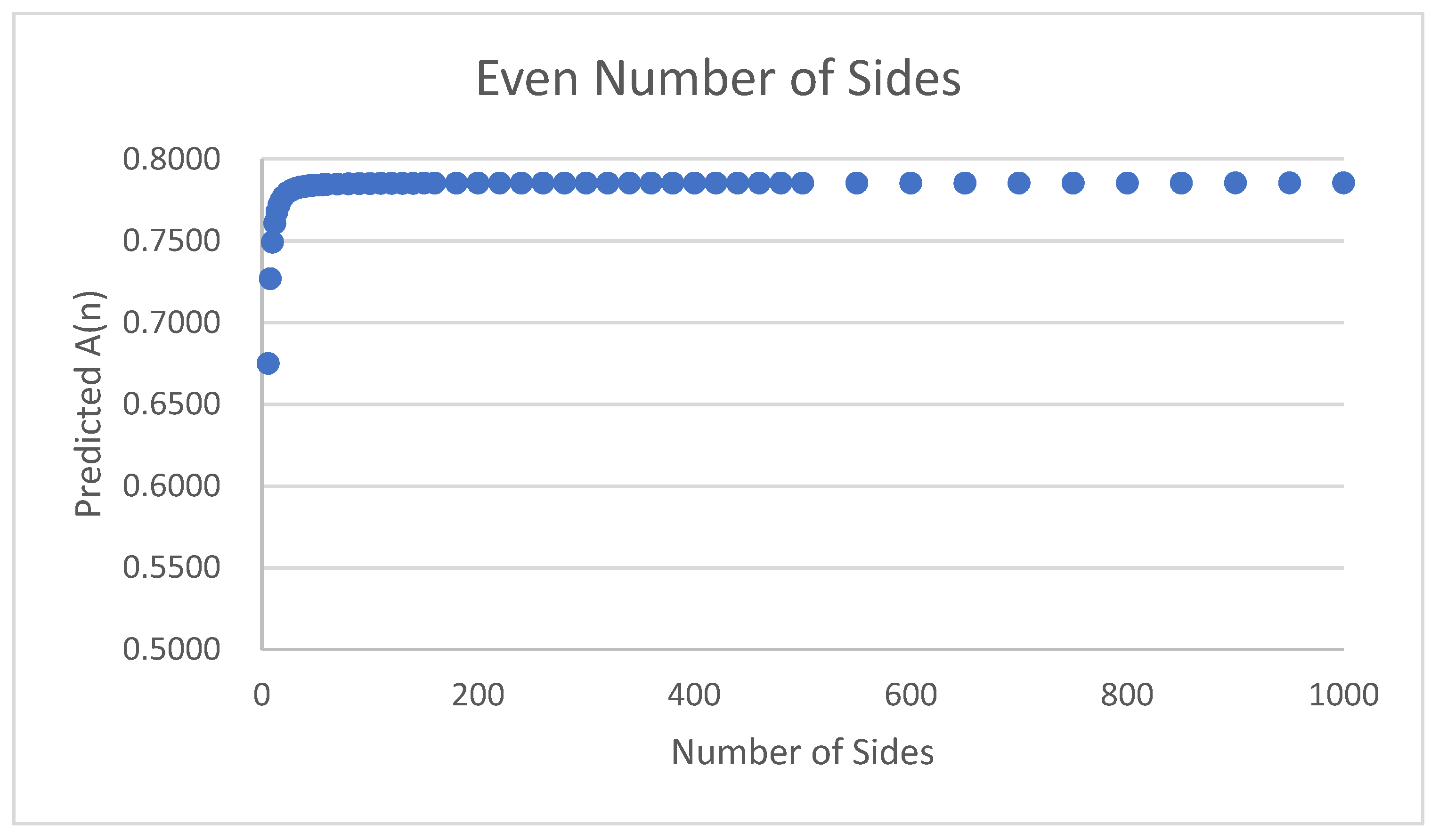
3. Numerical Results for Even Values $4\le n\le 1000$

The study summarized here was conducted on a laptop PC with the following specifications: Intel Core i7-7700 CPU @ 3.6 GHz (x-64 processor), 16.0 GB RAM, running under the Windows 10 Pro (64-bit) operating system.

To formulate directly scalable LSP model versions, we use the Mathematica model development environment (Wolfram Research, 2022a [9]). To handle these models numerically, we use the IPOPT local nonlinear optimization solver engine (Wächter and Laird, 2022 [10]) linked to Mathematica (Wolfram Research, 2022b [11]). The result analysis and visualization was also conducted in Mathematica.

Since IPOPT is a local scope solver, it requires an initial solution “guess:” hence, it greatly benefits from a good choice of that estimate. Considering the postulated structure of the LSP configurations to be found, for a given $n$ our initial angle settings are chosen as ${\theta }_i=i\left(\pi /n\right)$, for $1\le i\le n$, together with the initial polar radius settings $r_i=1$ for $1\le i\le n-1; r_n=0$

The numerical results obtained by using Mathematica and IPOPT are summarized below. Detailed $LSP\left(n\right)$ configurations (listing all decision variable values found and all constraints) can be optionally reported by our Mathematica code. All of the optimization results, with related analysis and visualization, are directly cited from the corresponding Mathematica (notebook) documents: thereby, our study is completely reproducible. The Mathematica notebook is available upon request from the authors.

Table 1. Mathematica-IPOPT numerical results for a selection of even values of $n$.

$\mathit{n}$	Decision Variables	Constraints	Runtime (Seconds)	Objective Function	Maximum Violation
4	6	5	0.03	0.500000	9.9636 × 10−9
6	10	14	0.03	0.674981 †	9.9432 × 10−9
8	14	27	0.05	0.726868 †	9.9236 × 10−9
10	18	44	0.06	0.749137 †	9.9046 × 10−9
12	22	65	0.08	0.760730 †	9.8855 × 10−9
14	26	90	0.11	0.767531 †	9.8663 × 10−9
16	30	119	0.15	0.771861 †	9.8472 × 10−9
18	34	152	0.17	0.774788 †	9.8296 × 10−9
20	38	189	0.23	0.776859 †	9.8101 × 10−9
24	46	275	0.32	0.779524 †	9.7801 × 10−9
28	54	377	0.45	0.781111 †	9.7647 × 10−9
32	62	495	0.68	0.782133 †	9.8456 × 10−9
36	70	629	0.82	0.782828 †	9.6522 × 10−9
40	78	779	1.05	0.783323 †	9.6132 × 10−9
44	86	945	1.34	0.783687 †	9.5741 × 10−9
48	94	1127	1.53	0.783964 †	9.5352 × 10−9
52	102	1325	1.85	0.784178 †	9.4967 × 10−9
56	110	1539	3.04	0.784252 *	9.6754 × 10−9
60	118	1769	3.34	0.784408 *	9.6548 × 10−9
70	138	2414	3.92	0.784729 †	9.3199 × 10−9
80	158	3159	4.98	0.784886 †	9.2227 × 10−9
90	178	4004	7.59	0.784994 †	9.1242 × 10−9
100	198	4949	9.44	0.785072 †	9.0264 × 10−9
110	218	5994	11.18	0.785129 †	8.9291 × 10−9
120	238	7139	14.21	0.785172 †	8.8306 × 10−9
130	258	8384	17.52	0.785205	8.7330 × 10−9
140	278	9729	21.39	0.785232	8.7013 × 10−9
150	298	11,174	25.11	0.785254	8.8048 × 10−9
160	318	12,719	29.16	0.785271	8.4389 × 10−9
180	358	16,109	52.43	0.785298	8.2424 × 10−9
200	398	19,899	51.31	0.785317	8.0460 × 10−9
220	438	24,089	64.43	0.785331	7.8491 × 10−9
240	478	28,679	81.60	0.785342	7.6515 × 10−9
260	518	33,669	97.73	0.785350	7.6285 × 10−9
280	558	39,059	118.77	0.785357	7.2925 × 10−9
300	598	44,849	142.19	0.785362	7.0879 × 10−9
320	638	51,039	170.00	0.785367	6.8695 × 10−9
340	678	57,629	202.27	0.785370	6.6526 × 10−9
360	718	64,619	235.11	0.785373	6.4506 × 10−9
380	758	72,009	269.55	0.785376	6.2473 × 10−9
400	798	79,799	316.30	0.785378	6.0432 × 10−9
420	838	87,989	363.92	0.785380	5.8990 × 10−9
440	878	96,579	393.75	0.785381	5.6483 × 10−9
460	918	105,569	464.32	0.785383	5.4201 × 10−9
480	958	114,959	514.01	0.785384	5.2503 × 10−9
500	998	124,749	577.96	0.785385	5.0971 × 10−9
550	1098	150,974	739.51	0.785387	4.4905 × 10−9
600	1198	179,699	948.26	0.785389	4.0205 × 10−9
650	1298	210,924	1228.83	0.785391	3.4442 × 10−9
700	1398	244,649	1460.31	0.785392	2.9080 × 10−9
750	1498	280,874	1857.58	0.785392	2.3883 × 10−9
800	1598	319,599	2342.02	0.785393	1.8715 × 10−9
850	1698	360,824	3177.43	0.785394	1.3518 × 10−9
900	1798	404,549	3846.06	0.785394	8.2861 × 10−10
950	1898	450,774	3721.68	0.785395 *	3.0161 × 10−10
1000	1998	499,499	5417.51	0.785395 *	0.0000 × 100

* Instances for which $A\left(n\right)$ ≤ A_n*. † Instances 6 ≤ n ≤ 120 for which A(n) ≥ A_n* as reported in Bingane (2020) [7].

summarizes our results for the selected even values of $4\le n\le 1000$. Since the solution times become rather substantial as $n$ increases, we report results only for a representative selection of even values; however, in principle we could handle all instances of $LSP\left(n\right)$, provably at least up to $n\le 1000$. For example (see Table 1), the runtime for $n=10$ is only $0.06$ s; for $n=100$ it is still just $9.44$ s; but for $n=1000$ it becomes $5417.51$ s. We did not conduct systematic tests to find the largest possible numerical instance that we could handle using Mathematica with IPOPT, noting that all of the modeling systems and optimization engines have their limitations, also depending on the hardware platform and other circumstances.

The legend used is self-explanatory, “Maximum violation” refers to the maximal constraint violation at the numerical optimal solution. One can verify the linear increase in the number of decision variables and the rapid quadratic increase in the number of constraints as a function of $n$ (recall the LSP model). The model instance for $n=1000$ has almost two thousand decision variables and nearly half a million constraints.

For even $n\ge 6$, it was shown in Mossinghoff (2006) [6] and Bingane (2022) [12] that the best known general lower bound is given by the diameter graph of an optimal $n$-polygon that has a cycle of length $n-1$ plus one additional edge from the remaining vertex. As such,

$$A\left(n\right)>{\underset{\_}{A}}_n=\frac{n-1}{2}\left(\sin \frac{\pi }{n-1}-\tan \frac{\pi }{2n-2}\right)+\sin \frac{\pi }{2n-2}-\frac{1}{2}\sin \frac{\pi }{n-1}.$$

(9)

Our results satisfy this general lower bound except for $A\left(56\right)$, $A\left(60\right)$, $A\left(950\right)$, and $A\left(1000\right)$. See Table 1. Indeed, equation (9) provides a very good general lower bound and it could be used as an additional constraint in the LSP optimization model. We note that Mossinghoff (2006) [6] and Bingane (2022) [12] obtained better asymptotic lower bounds by explicit instance constructions, which are not generally applicable as equation (9). In Table 1, we also indicate the instances $6\le n\le 120$ for which $A\left(n\right)\ge A_n^{*}$ (the optimal values of the maximal area problem for even $n$) as reported in Bingane (2020) [7].

Although Table 1 shows the optimized $A\left(n\right)$ values with only six digits after the decimal point, the reported precision in our detailed numerical tests (within Mathematica) is set to ten digits after the decimal point. To illustrate, our estimate for $A\left(1000\right)$ approximately equals $0.7853949284.$ Using such higher precision is in line with the required constraint satisfaction level, all in the order of ${10}^{-9}$ as shown in the table. The preset 10-digit precision also supports the in-depth comparisons with results obtained earlier. Specifically, our results are in close agreement with or surpass all of the best numerical results reported earlier, including Mossinghoff (2006) [6], Bingane (2020) [7], and Pintér (2021) [8], with reported comparisons to all earlier topical works known to us. Our modeling and optimization approach enables solving $LSP\left(n\right)$ instances for significantly higher values of $n$ than previously achieved by other researchers using a variety of modeling platforms and solver engines.

Figure 2 and Figure 3 display the solutions found for a selection of even sequences of $n$, showing all of the pairwise vertex connections. As expected, the configurations found quickly approach the circle, as $n$ increases.

Figure 4 summarizes the difference between the area $A\left(n\right)$ of the optimized polygon and $\pi /4$ as a function of $n$, on a loglog-plot scale. Our calculations reveal a small, but non-negligible difference: the numerically estimated slope of the plot for an even number of sides is approximately $-2.04618$.

We conclude the presentation of numerical results by emphasizing that the tightened LSP model offers advantages over the standard model. Specifically, IPOPT performs well on the tightened model, but it exhibits inferior performance on the standard model for values $6\le n\le 80$, as observed by Pintér (2021) [8]. Figure 5 illustrates the superior IPOPT performance on tightened LSP model-instances up to $n=300$, when compared to Figure 6 (standard LSP model with the same fixed starting solution as used in the tightened model) and Figure 7 (standard LSP model with $n$ random starting solutions). In the latter case, the solver runtimes also become longer; therefore, we conducted experiments only up to $n=100$.

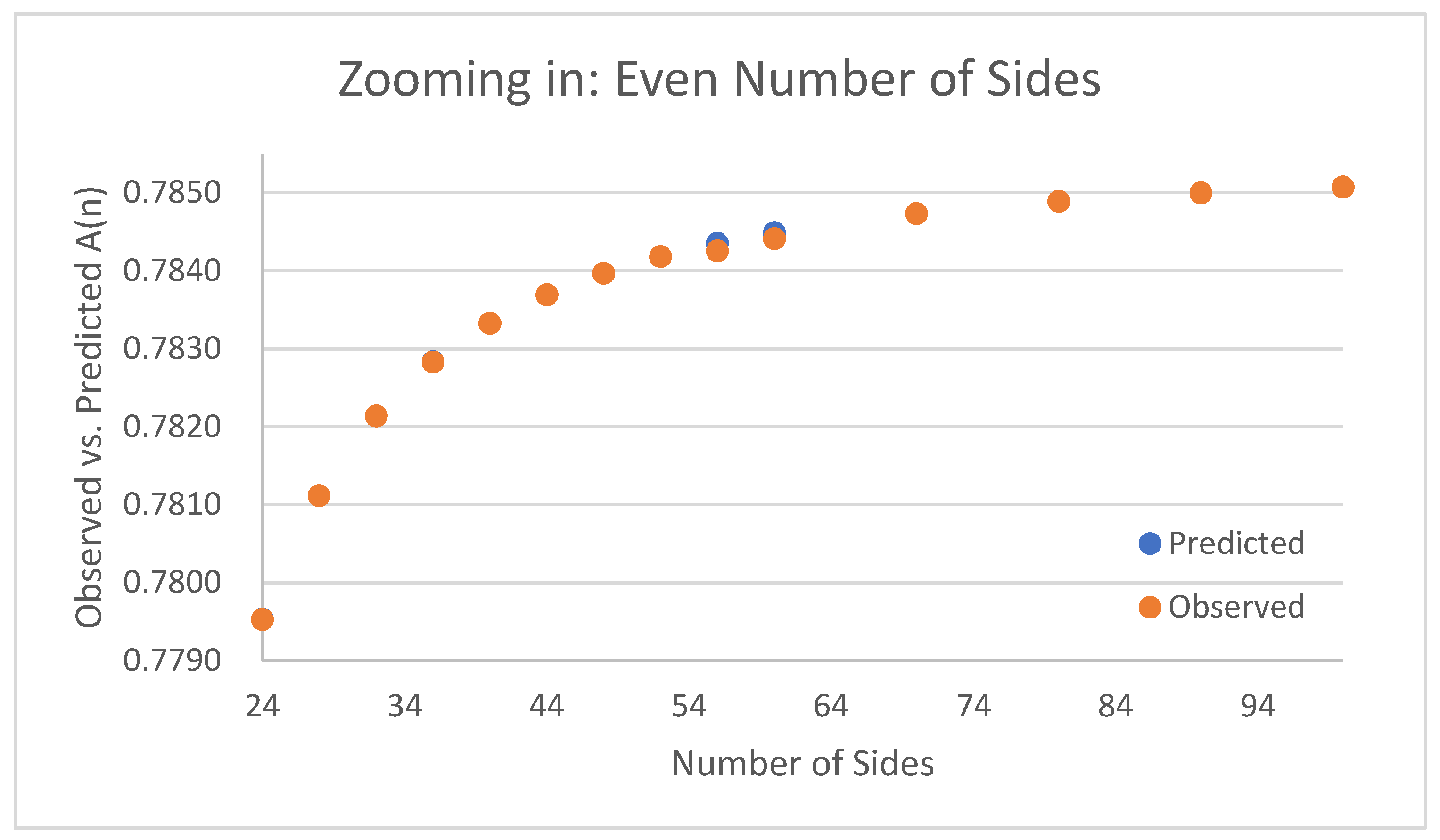
4. LSP(n) Regression Model for Even $n$

As it is known, and illustrated by Figure 2 and Figure 3, for large $n$ the optimal $LSP\left(n\right)$ configuration approaches the circle with unit diameter; hence the corresponding area limit is $A(\infty )=\pi /4~0.7853981634$. Comparing this limit value to our optimum estimate obtained for $A\left(1000\right)~0.7853949284$, the ratio $A\left(1000\right)/\left(\pi /4\right)$ approximately equals $0.9999958811$. Hence, our $A\left(1000\right)$ estimate already leads to a fairly close approximation of the limit value.

Based on this observation and using our numerical results, we developed the following regression model for even values of $n$.

$$A\left(n\right)~\frac{\pi }{4}-\frac{5{\pi }^3}{48n^2}-3.530190\left(\frac{1}{n^3}\right)-2.391836\left(\frac{1}{n^4}\right)-19.489487\left(\frac{1}{n^5}\right).$$

(10)

This regression model follows the form outlined in Foster and Szabo (2007) [13] and we received $p$-values (observed significance levels) well below 0.000001 for all coefficients. This finding indicates that we have very strong statistical evidence suggesting that the regression coefficients are all different from zero. Figure 8 depicts the predicted results using model (10).

Since the two sequences closely overlap, the preceding figure depicting observed vs. predicted $A\left(n\right)$ results become more useful when we zoom in and reduce the ranges considerably. In Figure 9, we display observed vs. predicted $A\left(n\right)$ results for $24\le n\le 100$ and $0.779\le A\left(n\right)\le 0.785$. The observed vs. predicted sequences appear visually different from each other only with high levels of magnification.

The regression model (10) can be used to directly estimate the selected values from the entire sequence $\left\{A\left(n\right)\right\}$, including larger values of $n$ which have not been studied earlier and may be out of the range of current optimization solver capabilities. For example,

$$A\left(2000\right)~0.7853973555,\hspace{1em}\hspace{1em}\hspace{1em}A\left(10000\right)~0.7853981311.$$

It is instructive to compare these estimates to $A(\infty )=\pi /4~0.7853981634$. Earlier numerical examples, with a different regression model based on results for even $6\le n\le 80$, are presented in Pintér (2021) [8].

5. Conclusions

Our study addresses the problem of numerically finding the sequence of the largest small $n$-polygons $LSP\left(n\right)$ with a unit diameter and maximal area of $A\left(n\right)$, in principle aiming for all of the even values of $n\ge 4$. This long-standing mathematical “puzzle” leads to an interesting class of nonlinear (global) optimization problems. We proposed a tightened LSP model and demonstrated its numerical advantages compared to the standard model. Using the Mathematica modeling environment with the IPOPT solver option, and our new initial solution estimate, we can find numerical solutions efficiently for a range of even values of $n$, up to $n\le 1000$. Our results compare well to all the best results reported earlier for significantly lower values of $n$. We also propose a regression model that enables the direct estimation of the optimal area sequence $\left\{A\left(n\right)\right\}$, for even values of $n$.

The LSP problem-class is one of those entertaining “puzzles” that can be described in a few words yet lead to surprisingly hard theoretical and numerical challenges. Therefore, this model-class—similarly to many other scientifically important configuration design models—can also be used in software benchmarking tests. We think that such problems serve as a significant addendum to the collection of (well-frequented, and often much simpler) unconstrained or box-constrained test problems. For further examples of increasingly hard-to-solve object configuration models, we refer to some of our studies: consult, e.g., Castillo et al. (2008) [14], Pintér et al. (2017) [15], Kampas et al. (2019) [16], Kampas et al. (2020) [17].

References

1. Reinhardt, K. Extremale polygone gegebenen durchmessers. Jahresber. Dtsch. Math. Ver. 1922, 31, 251–270. [Google Scholar]
2. Graham, R.L. The largest small hexagon. J. Comb. Theory Ser. A 1975, 18, 165–170. [Google Scholar] [CrossRef] [Green Version]
3. Audet, C.; Hansen, P.; Messine, F.; Xiong, J. The largest small octagon. J. Comb. Theory Ser. A 2002, 98, 46–59. [Google Scholar] [CrossRef] [Green Version]
4. Audet, C.; Hansen, P.; Svrtan, D. Using symbolic calculations to determine largest small polygons. J. Glob. Optim. 2021, 81, 261–268. [Google Scholar] [CrossRef]
5. Henrion, D.; Messine, F. Finding largest small polygons with GloptiPoly. J. Glob. Optim. 2013, 56, 1017–1028. [Google Scholar] [CrossRef] [Green Version]
6. Mossinghoff, M.J. Isodiametric problems for polygons. Discret. Comput. Geom. 2006, 36, 363–379. [Google Scholar] [CrossRef] [Green Version]
7. Bingane, C. Largest small polygons: A sequential convex optimization approach. arXiv 2020, arXiv:2009.07893. Available online: https://arxiv.org/abs/2009.07893 (accessed on 14 January 2022).
8. Pintér, J.D. Largest small n-polygons: Numerical optimum estimates for n ≥ 6. In Recent Developments in Numerical Analysis and Optimization (NAO-V, Muscat, Oman, January 2020); Al-Baali, M., Grandinetti, L., Purnama, A., Eds.; Springer Nature: New York, NY, USA, 2021; pp. 231–247. [Google Scholar]
9. Wolfram Research. Mathematica, Current Release 13.0 (as of January 2022); Wolfram Research: Champaign, IL, USA, 2022. [Google Scholar]
10. Wächter, A.; Laird, C. IPOPT (Interior Point Optimizer), an Open Source Software Package for Large-Scale Nonlinear Optimization. Available online: https://github.com/coin-or/Ipopt (accessed on 14 January 2022).
11. Wolfram Research (2022b), Optimizing with IPOPT. Available online: https://reference.wolfram.com/language/IPOPTLink/tutorial/OptimizingWithIPOPT.html (accessed on 14 January 2022).
12. Bingane, C. Tight bounds on the maximal area of small polygons: Improved Mossinghoff polygons. Discret. Comput. Geom. 2022. [Google Scholar] [CrossRef]
13. Foster, J.; Szabo, T. Diameter graphs of polygons and the proof of a conjecture of Graham. J. Comb. Theory Ser. A 2007, 114, 1515–1525. [Google Scholar] [CrossRef] [Green Version]
14. Castillo, I.; Kampas, F.J.; Pintér, J.D. Solving circle packing problems by global optimization: Numerical results and industrial applications. Eur. J. Oper. Res. 2008, 191, 786–802. [Google Scholar] [CrossRef]
15. Pintér, J.D.; Kampas, F.J.; Castillo, I. Globally optimized packings of non-uniform size spheres in Rd: A computational study. Optim. Lett. 2017, 12, 585–613. [Google Scholar] [CrossRef]
16. Kampas, F.J.; Castillo, I.; Pintér, J.D. Optimized ellipse packings in regular polygons. Optim. Lett. 2019, 13, 1583–1613. [Google Scholar] [CrossRef]
17. Kampas, F.J.; Pintér, J.D.; Castillo, I. Packing ovals in optimized regular polygons. J. Glob. Optim. 2020, 77, 175–196. [Google Scholar] [CrossRef] [Green Version]
Figure 1. Our conjectured largest small polygons L S P ( 6 ) and L S P ( 18 ) .
Mca 27 00042 g001
Figure 2. Conjectured largest small polygons L S P ( n ) for n = 6 , 8 , 10 , 12 , 14 , 16 , 18 , 20 .
Mca 27 00042 g002
Figure 3. Conjectured largest small polygons L S P ( n ) for n = 30 , 40 , 50 , 60 , 70 , 80 , 90 , 100 .
Mca 27 00042 g003
Figure 4. Difference between the area A ( n ) of the optimized polygon and π / 4 , for selected even values 4 n 150 .
Mca 27 00042 g004
Figure 5. IPOPT performance on tightened LSP model-instances up to n = 300 . Difference between the area A ( n )   of the optimized polygon and π / 4 .
Mca 27 00042 g005
Figure 6. IPOPT performance on standard LSP model-instances, with the proposed starting solution, up to n = 300 . Difference between the area A ( n )   of the optimized polygon and π / 4 .
Mca 27 00042 g006
Figure 7. IPOPT performance on standard LSP model-instances, with random starting solutions up to n = 100 . Difference between the area A ( n )   of the optimized polygon and π / 4 .
Mca 27 00042 g007
Figure 8. The nonlinear regression model (10) predicting A ( n ) shown for even 4 n 1000 .
Mca 27 00042 g008
Figure 9. Zooming in: observed vs. predicted A ( n ) results applying the regression model (10) for even 24 n 100 .
Mca 27 00042 g009