
CFD Simulation for Estimating Efficiency of PBCF Installed on a 176K Bulk Carrier under Both POW and Self-Propulsion Conditions


Abstract
:1. Introduction
2. Test Methods
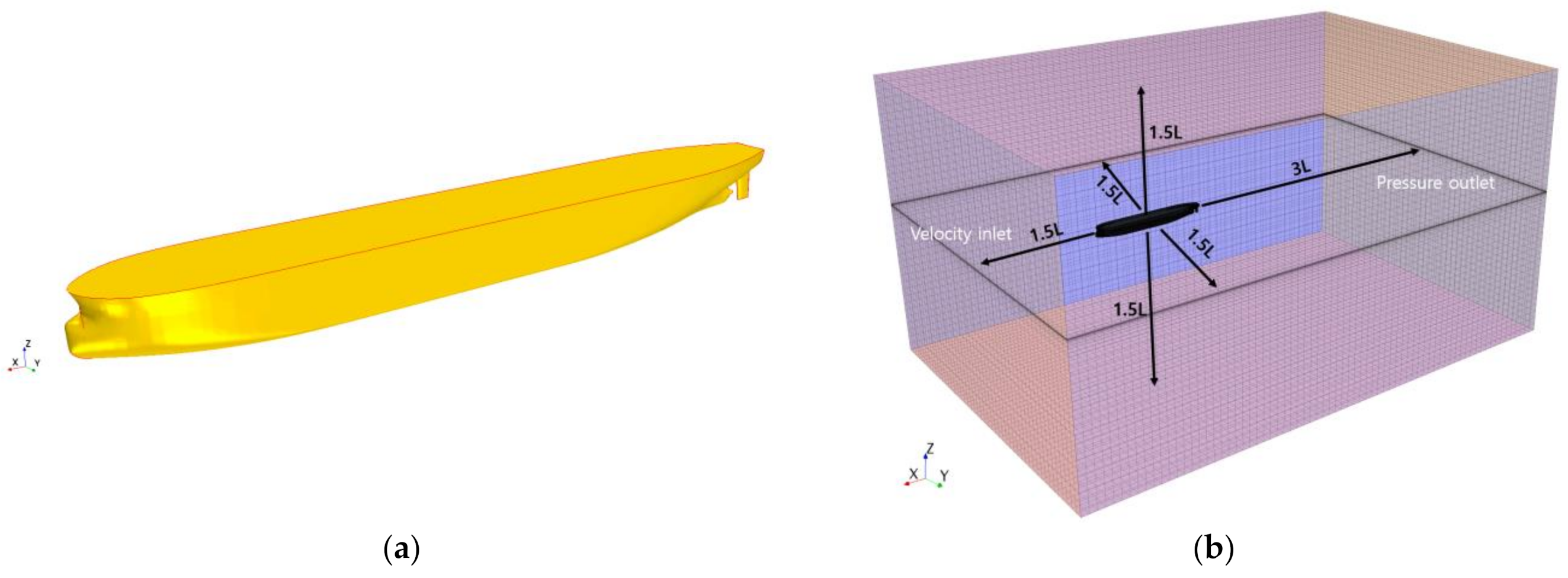
2.1. Resistance Test
2.2. POW Test
2.3. Reversed POW Test
2.4. Self-Propulsion Test
2.5. Numerical Modeling
2.5.1. Governing Equations
2.5.2. Turbulence Model
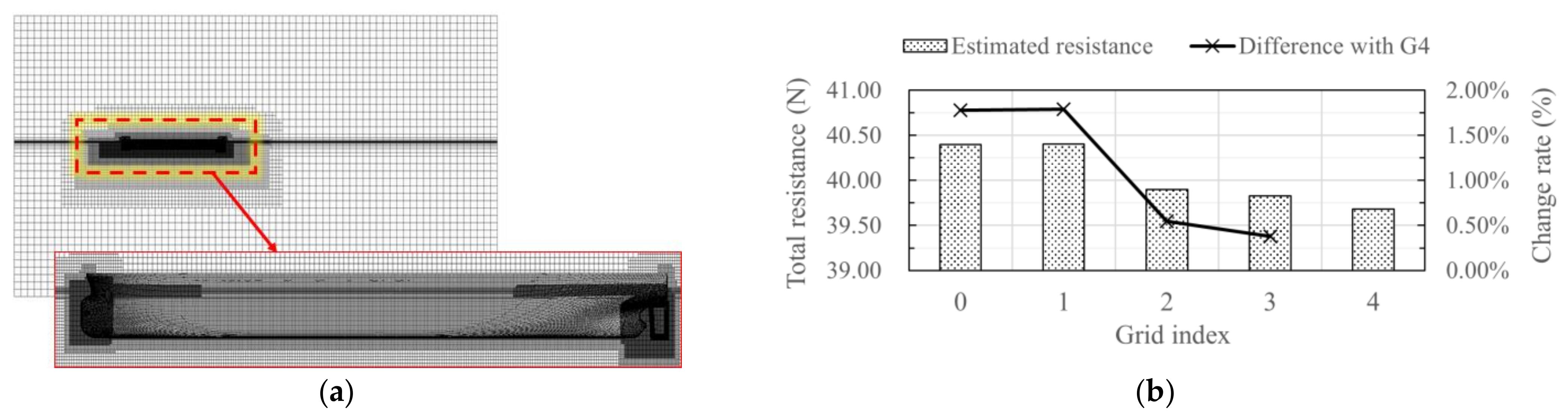
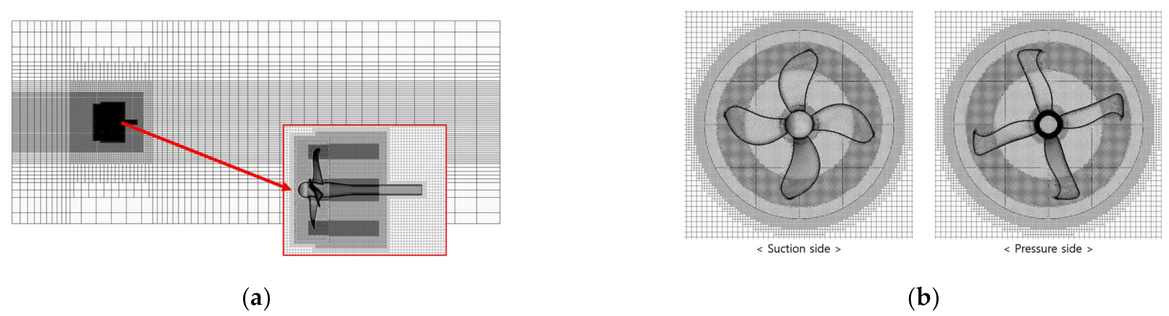
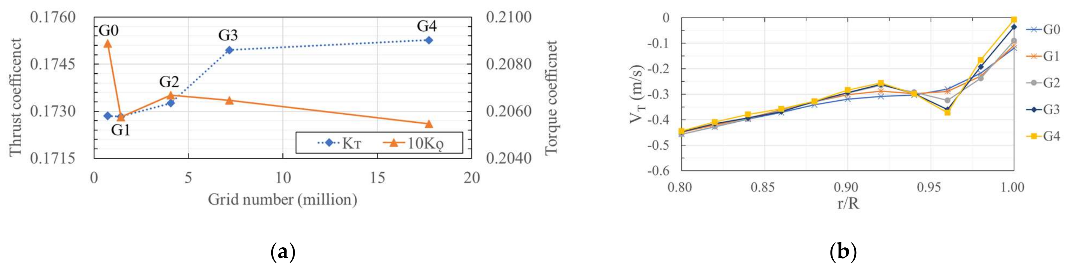
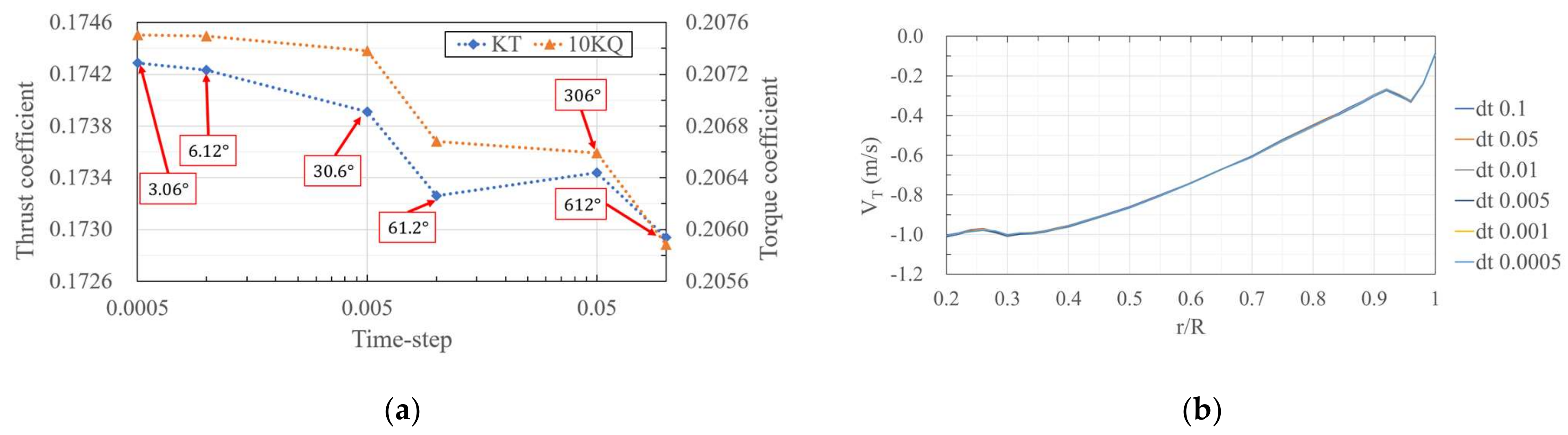
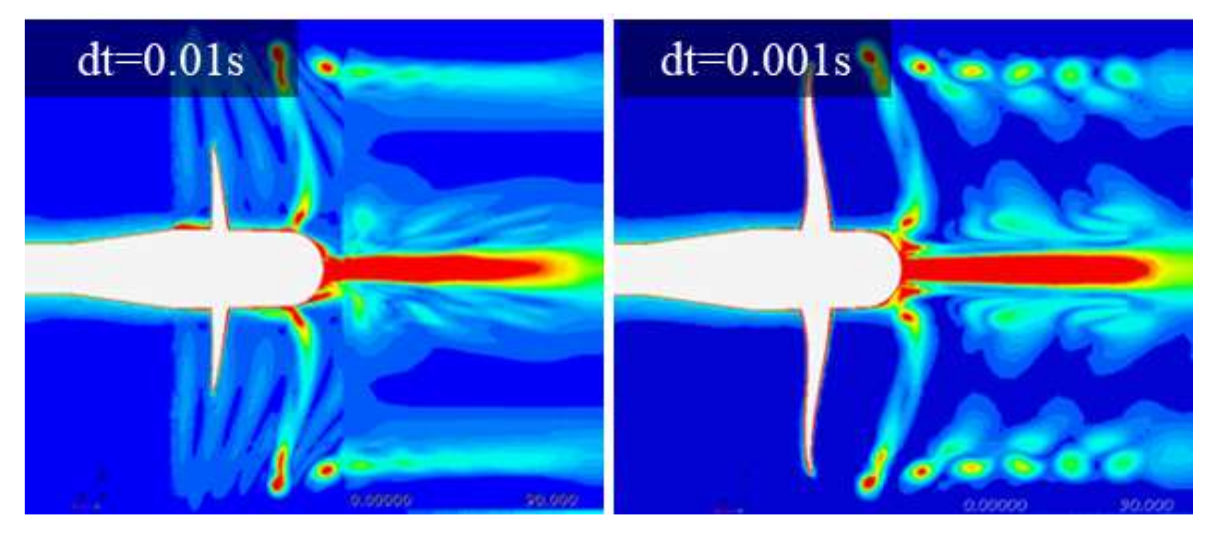
2.5.3. Grid Systems and Numerical Modeling
3. Resistance Test
3.1. Simulation Condition
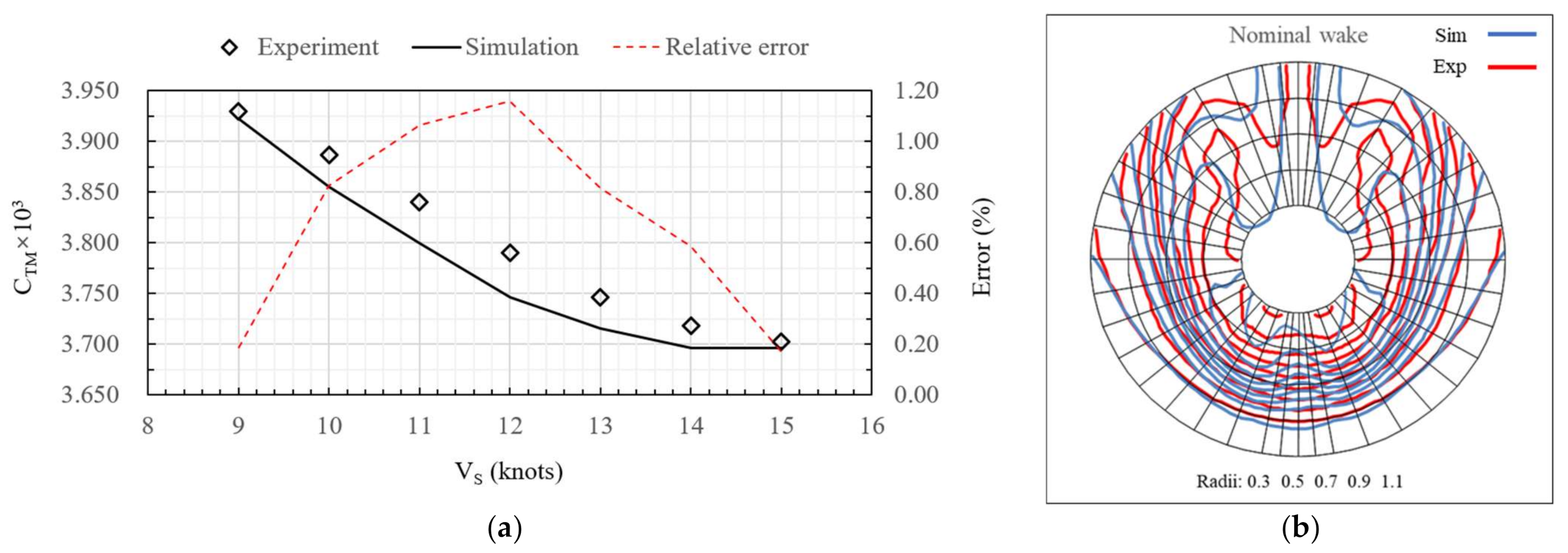
3.2. Simulation Results and Verification
4. POW Test
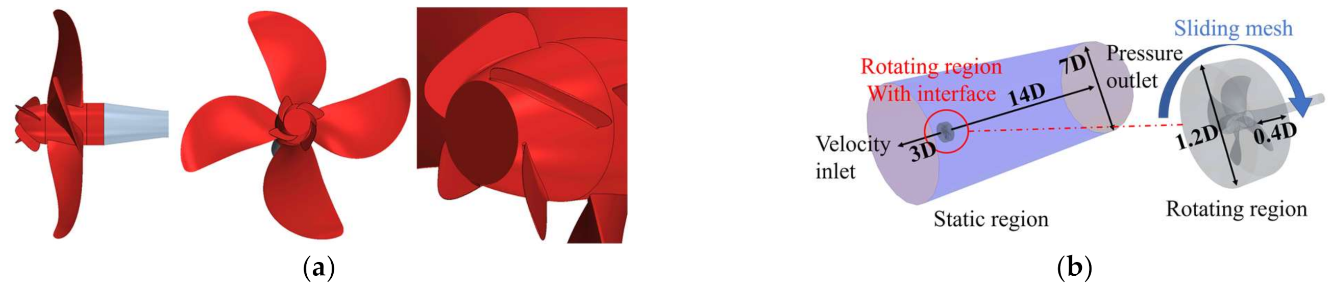
4.1. Simulation Condition
4.2. Simulation Results and PBCF Efficiency Analysis
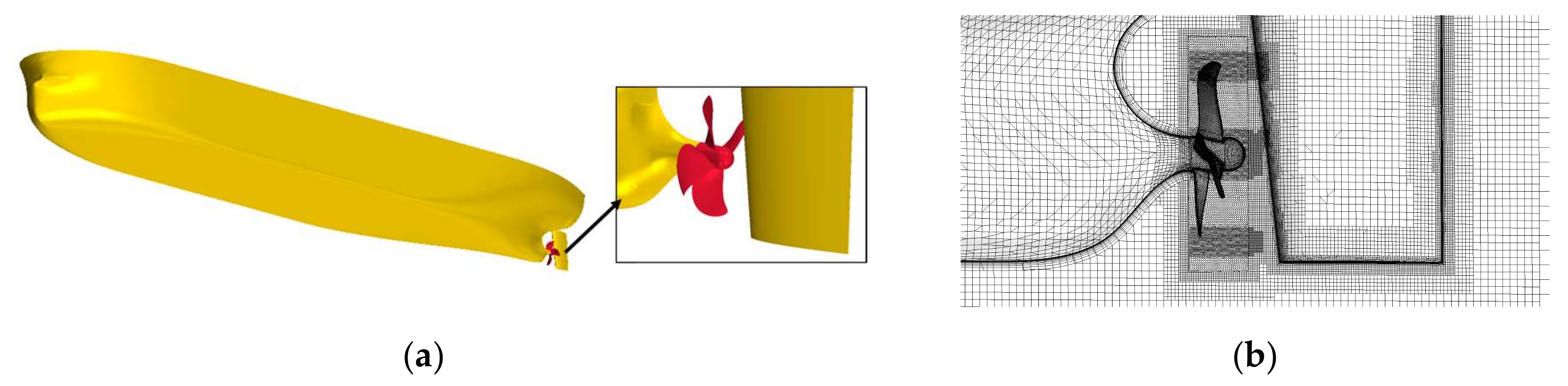
5. Self-Propulsion Test
5.1. Simulation Condition
5.2. Simulation Results and Verification
6. Conclusions
- In the resistance test, the total resistance of the 176K bulk carrier was estimated in the experiment and the simulation, showing an relative error of up to 1.2% according to the ship speed. In addition, the nominal wake was estimated similarly in the experiment and the simulation. Thus, simulation settings for self-propulsion test were designed appropriately.
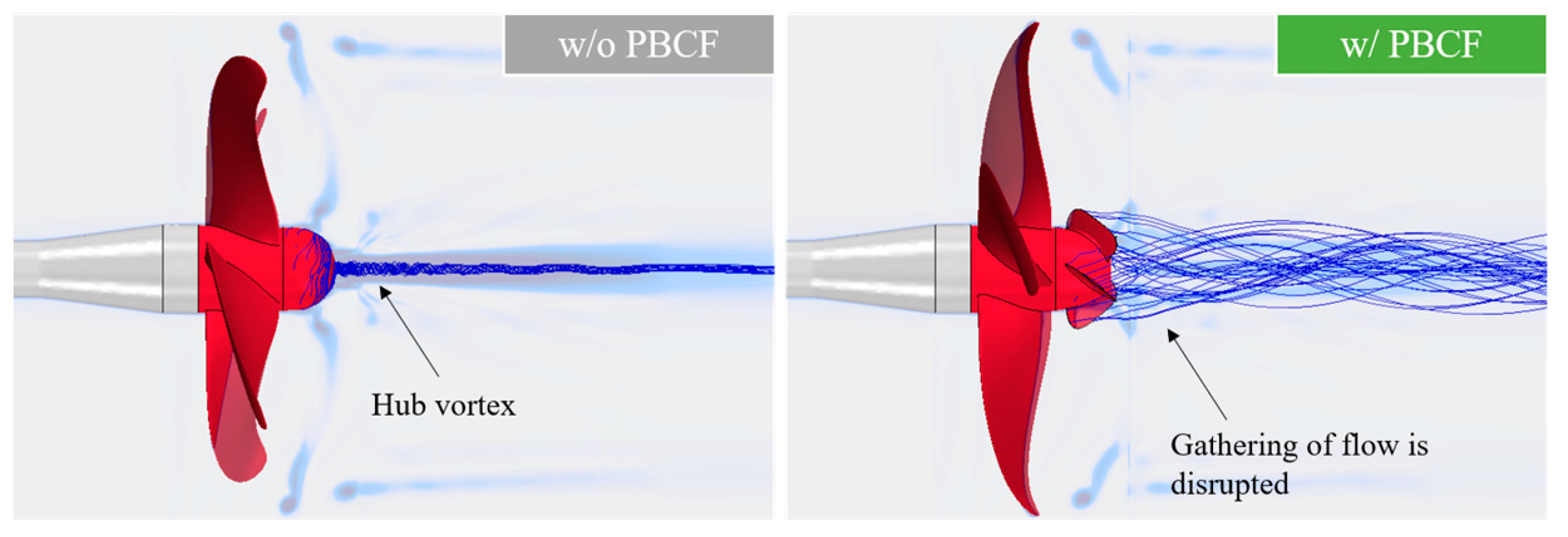
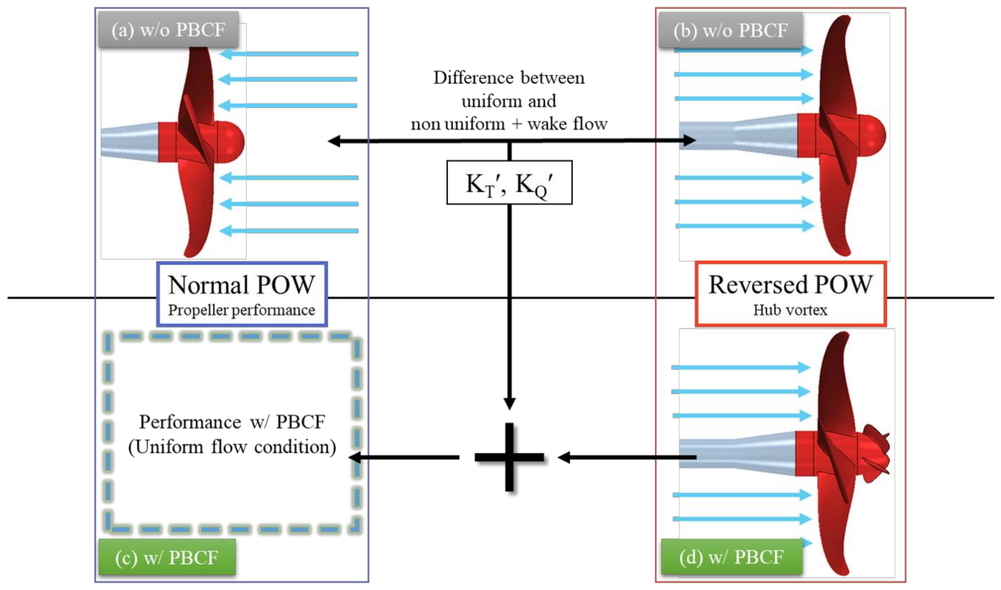
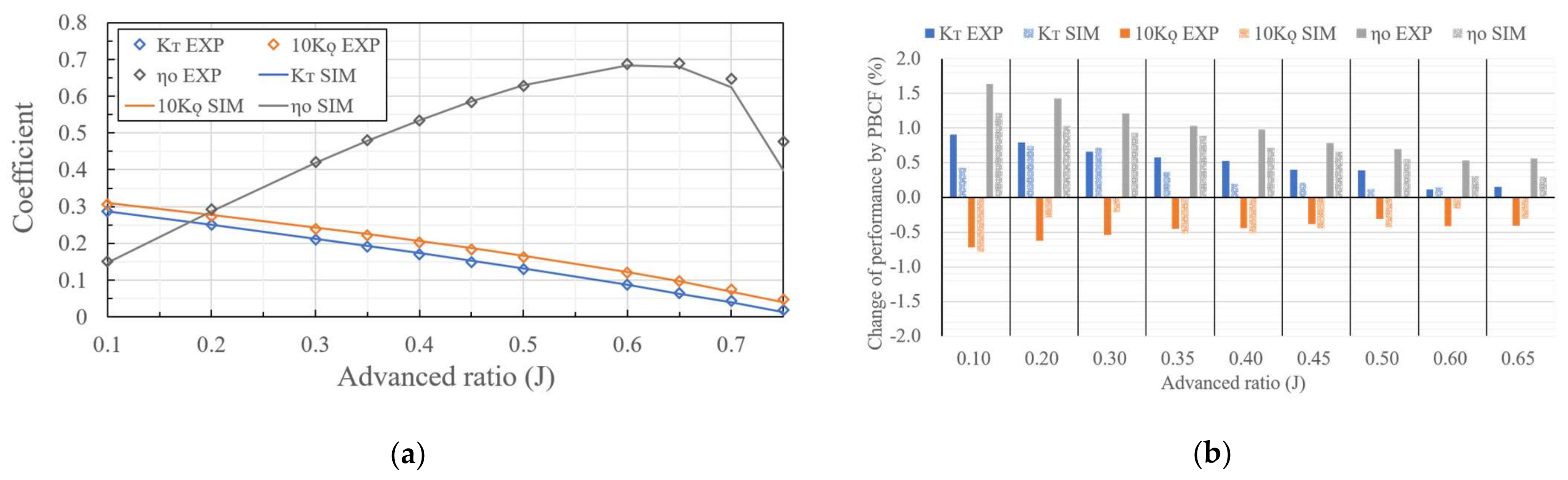
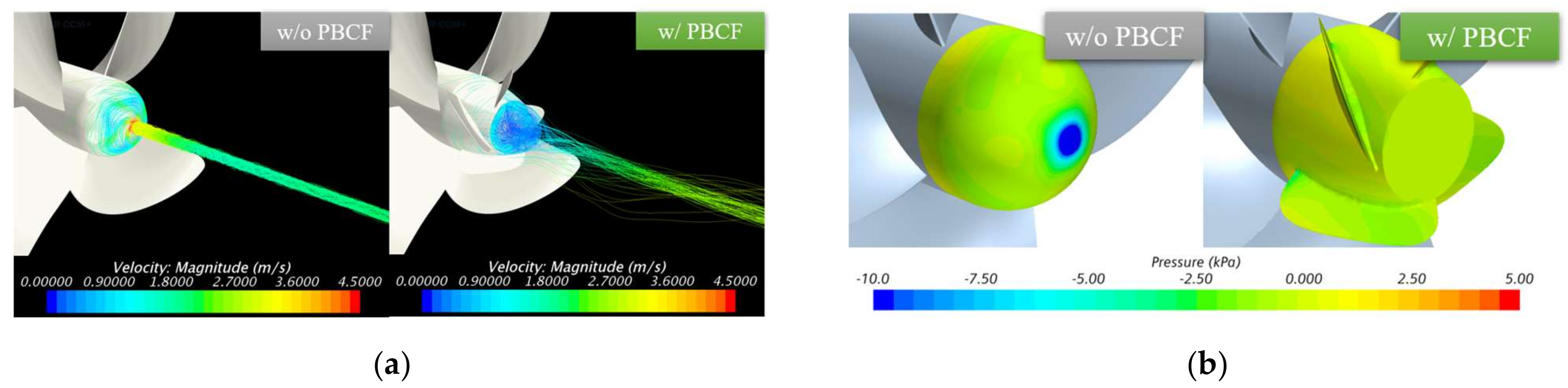
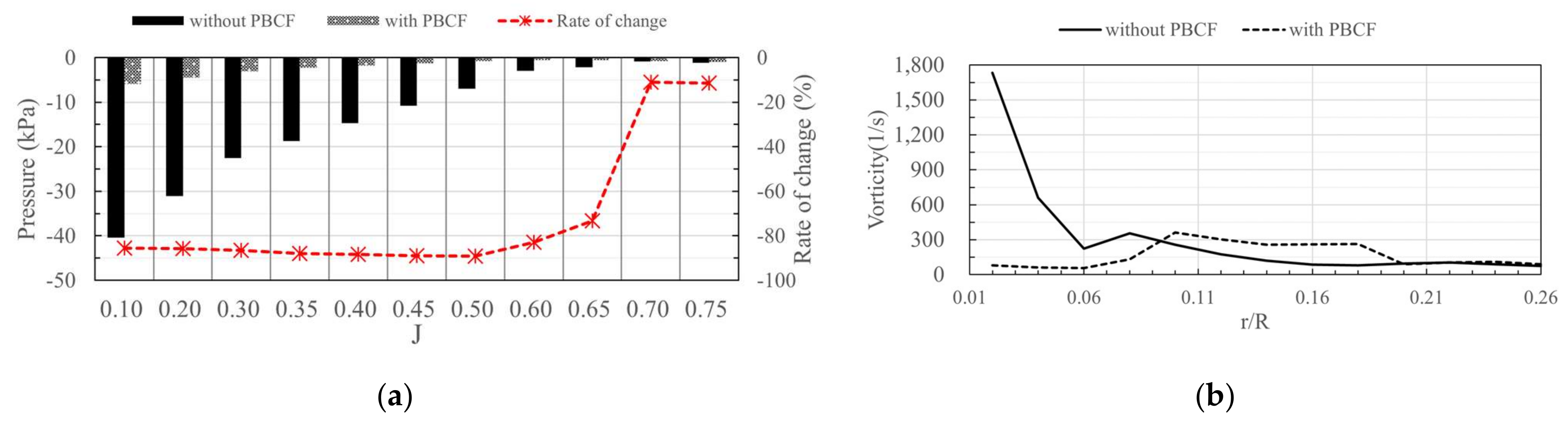
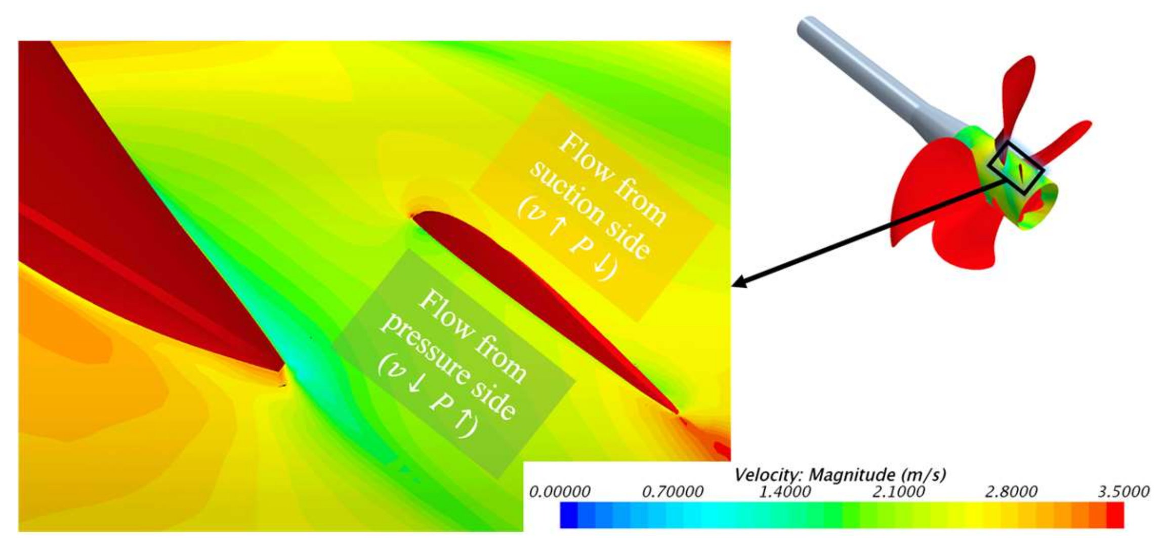
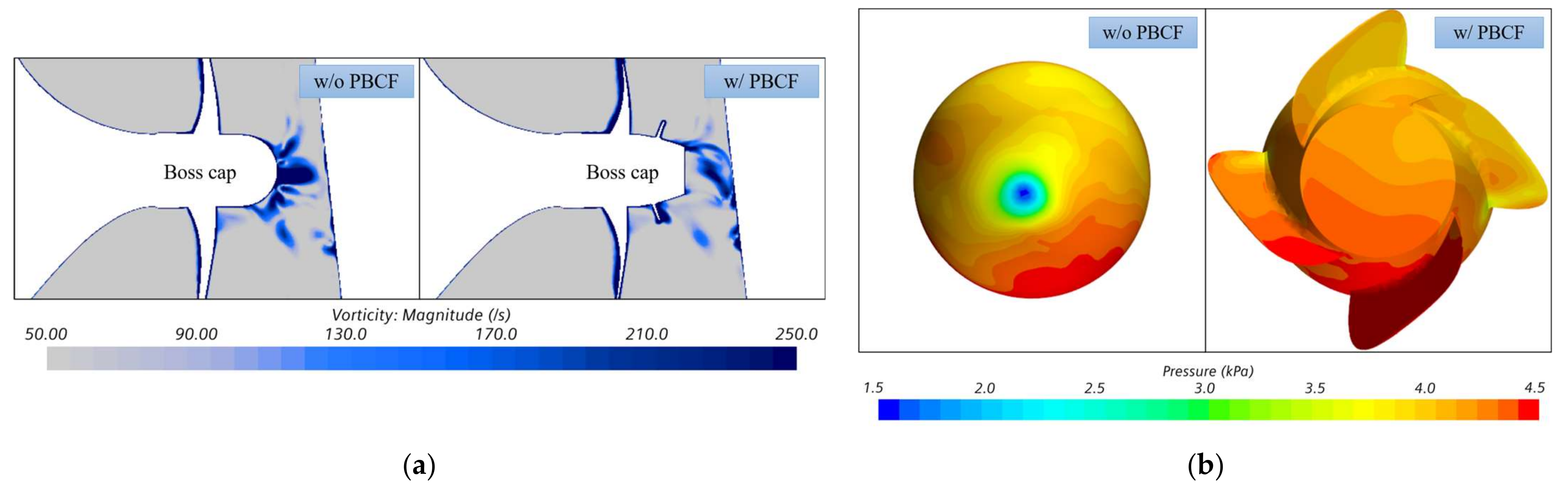
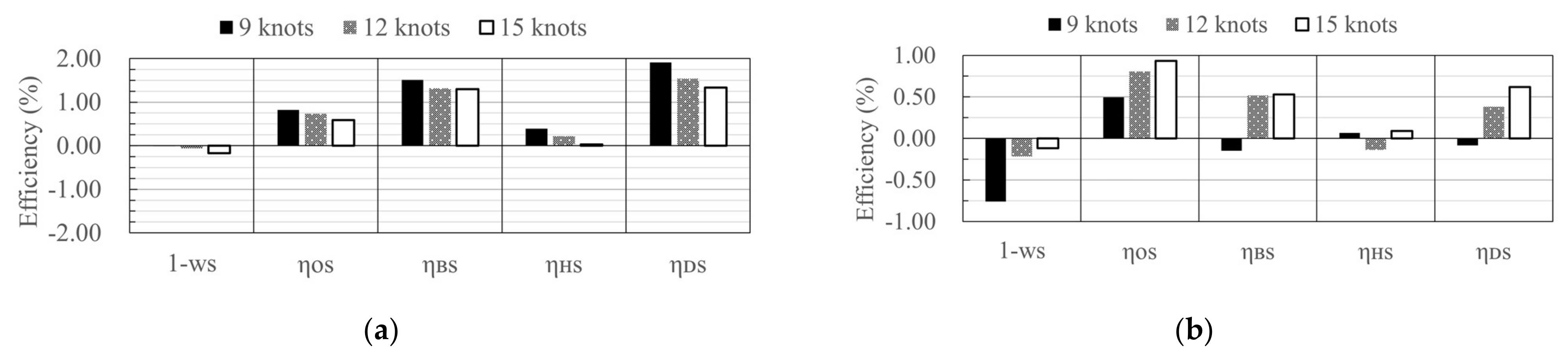
- In the POW test, the POW curve with or without PBCF was estimated and a correction method was used to obtain the propeller open water performance when the PBCF was installed under the POW condition. The POW curve showed only a relative error of 2% or less between the experiment and the simulation except that the advance ratio was very high. In the POW condition, the PBCF effect was similar to the result shown in the experiment. The thrust increased by about 0.5% and the torque was decreased by 0.4%, so that the propeller open water efficiency was increased by about 1%. In the simulation result, the mechanism of PBCF was investigated using a flow field analysis. A breakdown of the hub vortex after installing PBCF was successfully observed.
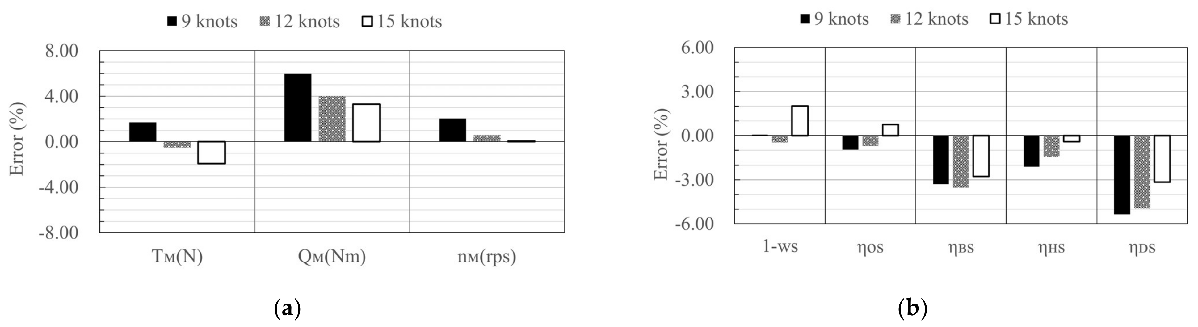
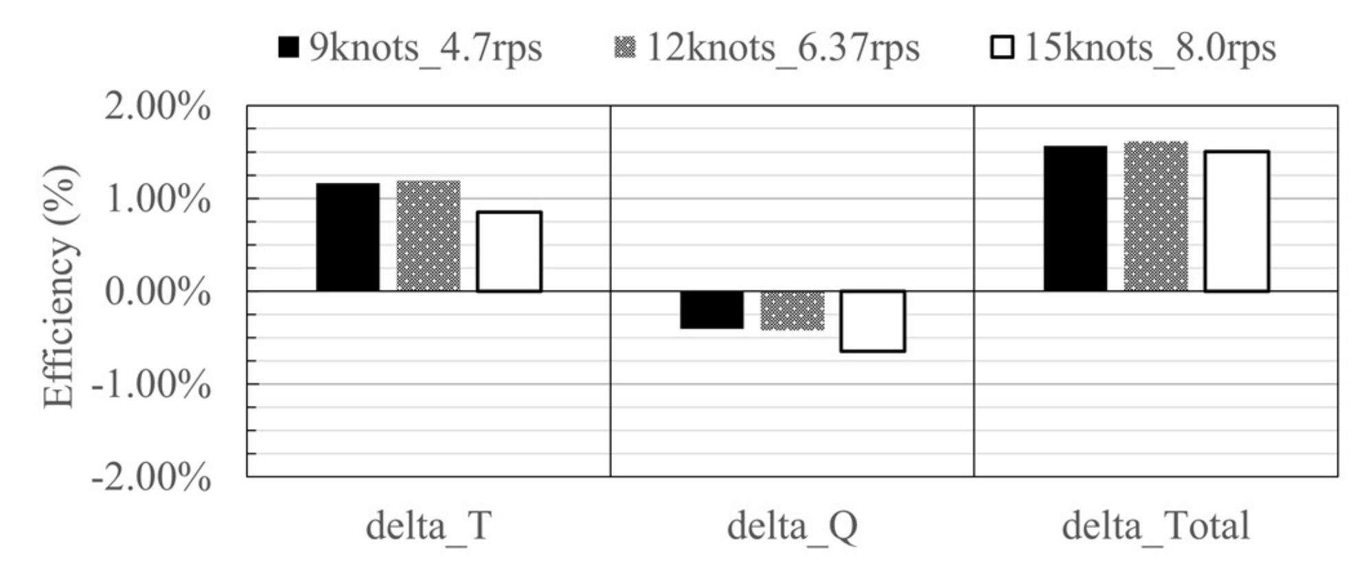
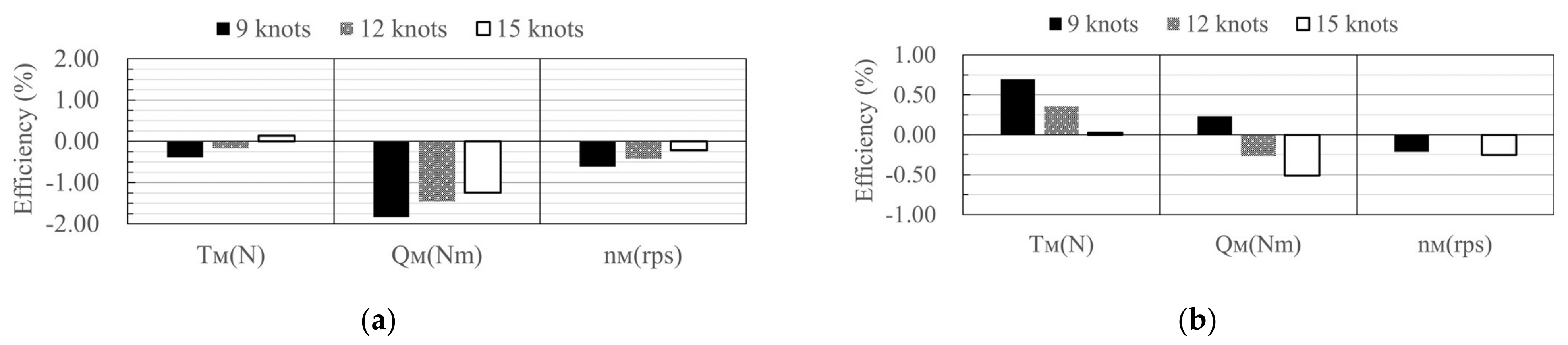
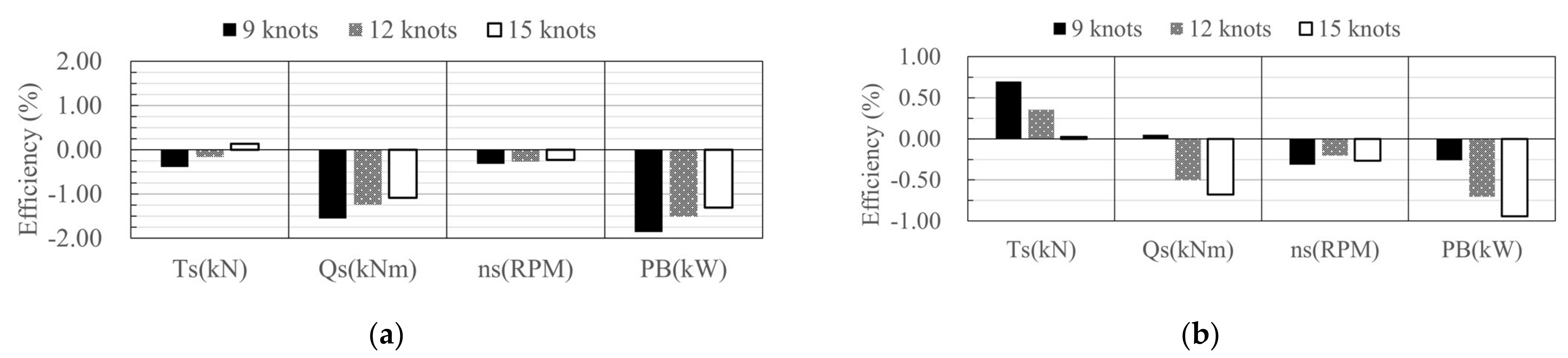
- In the self-propulsion test, propulsion performance at self-propulsion point in the simulation were found to be very similar to those in the experiment, although the torque had a remarkably large relative error of 3–6%. Changes of the propulsion performance due to PBCF were relatively consistent according to ship speed in the simulation. The trend of the PBCF effect in the self-propulsion test was very similar to the observation in the POW test. On the other hand, in the experiment, the PBCF effect at each speed did not show a consistent trend. The reason was that the amount of change in the performance by PBCF was about 0.5–1%, making it difficult to precisely measure in the model test. However, in the experiment with PBCF, the performance at the self-propulsion point also changed in a positive direction. Finally, it was found that, with PBCF, the BHP decreased by 1.5% in the simulation and by 0.5% level in the experiment.
- Exact estimation of PBCF efficiency from the model test, full-scale measurement, and sea-trial is difficult because of various environmental condition. Model-scale simulation shows a consistent trend for the PBCF effect. However, there is a fundamental problem about the scale effect. Thus, for more accurately understand the effect of PBCF at full-scale, a full-scale simulation will be required eventually.
Author Contributions
Funding
Institutional Review Board Statement
Informed Consent Statement
Conflicts of Interest
References
- Smith, T.W.P.; Jalkanen, J.P.; Anderson, B.A.; Corbett, J.J.; Faber, J.; Hanayama, S.; O’Keeffe, E.; Parker, S.; Johansson, L.; Aldous, L.; et al. Third IMO Greenhouse Gas Study; International Maritime Organization: London, UK, 2015; Micropress Printers: Suffolk, UK, 2015. [Google Scholar]
- Olmer, N.; Comer, B.; Roy, B.; Mao, X.; Rutherford, D. Greenhouse Gas Emissions from Global Shipping, 2013–2015 Detailed Methodology; The International Council on Clean Transportation: Washington, DC, USA, 2017. [Google Scholar]
- Cames, M.; Graichen, J.; Siemons, A.; Cook, V. Emission reduction targets for international aviation and shipping. In Policy Department A: Economic and Scientific Policy; European Parliament: Brussels, Belgium, 2015. [Google Scholar]
- IMO. Resolution MEPC.203(62). In Amendments to the Annex of the Protocol of 1997 to Amend the International Convention for the Prevention of Pollution from Ships, 1973, as Modified by the Protocol of 1978 Relating Thereto; IMO: London, UK, 2011. [Google Scholar]
- Kawamura, T.; Ouchi, K.; Nojiri, T. Model and full scale CFD analysis of propeller boss cap fins (PBCF). J. Mar. Sci. Technol. 2012, 17, 469–480. [Google Scholar] [CrossRef]
- Nojiri, T.; Ishii, N.; Kai, H. Energy saving technology of PBCF (Propeller Boss Cap Fins) and its evolution. J. Jpn. Inst. Mar. Eng. 2011, 46, 350–358. [Google Scholar] [CrossRef]
- MOL Techno-Trade, Ltd. Energy-Saving Propeller Boss Cap Fins System Reaches Major Milestone—Orders Received for 3000 Vessels. Available online: https://www.mol.co.jp/en/pr/2015/15033.html (accessed on 14 October 2018).
- Ouchi, K.; Ogura, M.; Kono, Y.; Orito, H.; Shiotsu, T.; Tamashima, M.; Koizuka, H. A research and development of PBCF (propeller boss cap fins). J. Soc. Nav. Archit. Jpn. 1988, 1988, 66–78. [Google Scholar] [CrossRef]
- Ghassemi, H.; Mardan, A.; Ardeshir, A. Numerical analysis of hub effect on hydrodynamic performance of propellers with inclusion of PBCF to equalize the induced velocity. Pol. Marit. Res. 2012, 19, 17–24. [Google Scholar] [CrossRef]
- Druckenbrod, M.; Wang, K.; Greitsch, L.; Heinke, H.J.; Abdel-Maksoud, M. Development of hub caps fitted with PBCF. In Proceedings of the Fourth International Symposium on Marine Propulsors, Austin, TX, USA, 31 May–4 June 2015. [Google Scholar]
- Katayama, K.; Okada, Y.; Okazaki, A. Optimization of the Propeller with ECO-Cap by CFD. In Proceedings of the Fourth International Symposium on Marine Propulsors, Austin, TX, USA, 31 May–4 June 2015. [Google Scholar]
- Park, H.J.; Kim, K.S.; Suh, S.; Park, I.R. CFD Analysis of Marine Propeller-Hub Vortex Control Device Interaction. J. Soc. Nav. Archit. Korea 2016, 53, 266–274. [Google Scholar] [CrossRef] [Green Version]
- Mizzi, K.; Demirel, Y.K.; Banks, C.; Turan, O.; Kaklis, P.; Atlar, M. Design optimisation of Propeller Boss Cap Fins for enhanced propeller performance. Appl. Ocean Res. 2017, 62, 210–222. [Google Scholar] [CrossRef] [Green Version]
- Kim, E.K.; Lee, K.K.; Cho, K.H. A Study on the Performance Comparison of Energy Saving Devices for Handy-size Bulk Carrier. J. Korean Soc. Mar. Eng. 2015, 39, 1–7. [Google Scholar]
- ITTC. 1978 ITTC Performance Prediction Method. In ITTC Report 7.5-02-03-01.4; ITTC: Zürich, Switzerland, 2017. [Google Scholar]
- Carrica, P.M.; Castro, A.M.; Stern, F. Self-Propulsion computations using a speed controller and a discretized propeller with dynamic overset grids. J. Mar. Sci. Technol. 2010, 15, 316–330. [Google Scholar] [CrossRef]
- Kim, J.; Park, I.R.; Kim, K.S.; Van, S.H. RANS computation of turbulent free surface flow around a self-propelled KLNG carrier. J. Soc. Nav. Archit. Korea 2005, 42, 583–592. [Google Scholar]
- Phillips, A.B.; Turnock, S.R.; Furlong, M. Evaluation of maneuvering coefficients of a self-propelled ship using a blade element momentum propeller model coupled to a Reynolds averaged Navier Stokes flow solver. Ocean Eng. 2009, 36, 1217–1225. [Google Scholar] [CrossRef] [Green Version]
- Choi, J.E.; Min, K.S.; Kim, J.H.; Lee, S.B.; Seo, H.W. Resistance and propulsion characteristics of various commercial ships based on CFD results. Ocean Eng. 2010, 37, 549–566. [Google Scholar] [CrossRef]
- Lee, J.H.; Park, B.J.; Rhee, S.H. Ship Resistance and Propulsion Performance Test Using Hybrid Mesh and Sliding Mesh. J. Comput. Fluids Eng. 2010, 15, 81–87. [Google Scholar]
- Bugalski, T.; Hoffmann, P. Numerical simulation of the self-propulsion model tests. In Proceedings of the Second International Symposium on Marine Propulsors, Hamburg, Germany, 15–17 June 2011. [Google Scholar]
- Villa, D.; Gaggero, S.; Brizzolara, S. Ship Self Propulsion with different CFD methods: From actuator disk to viscous inviscid unsteady coupled solvers. In Proceedings of the 10th International Conference on Hydrodynamics, Saint Petersburg, Russia, 1–4 October 2012. [Google Scholar]
- Krasilnikov, V.I. Self-propulsion RANS computations with a single-screw container ship. In Proceedings of the Third International Symposium on Marine Propulsors, Tasmania, Australia, 5–8 May 2013. [Google Scholar]
- Lungu, A. Numerical simulation of the resistance and self-propulsion model tests. In Proceedings of the ASME 2018 37th International Conference on Ocean, Offshore and Arctic Engineering, Madrid, Spain, 17–22 June 2018. [Google Scholar]
- Kuiper, G. Cavitation Inception on Ship Propeller Models. Ph.D. Thesis, Delft University of Technology, Delft, The Netherlands, 11 March 1981. [Google Scholar]
- Sasajima, T. A Study on the Propeller Surface Flow in Open and Behind Condition. In Proceedings of the 14th ITTC Contribution to Performance Committee, Ottawa, ON, Canada, 11 September 1975; Volume 3, p. 711. [Google Scholar]
- Tsuda, T.; Konishi, S. Effect of Reynolds Number on Propeller Characteristics. In Note to the ITTC Propeller Committee; ITTC: Zürich, Switzerland, 1978. [Google Scholar]
- ITTC. Final Report of the Propulsor Committee. In Proceedings of the 20th ITTC, San Francisco, CA, USA, 19–25 September 1993. [Google Scholar]
- Castelli, E.B.; Raciti, M.; Grandi, G. Numerical Analysis of Laminar to Turbulent Transition on the DU91-W2-250 airfoil. Int. J. Mech. Aerosp. Ind. Mechatron. Manuf. Eng. 2012, 6, 717–724. [Google Scholar]
- Wang, X.; Walters, K. Computational analysis of marine-propeller performance using transition-sensitive turbulence modeling. J. Fluids Eng. 2012, 134, 071107. [Google Scholar] [CrossRef] [Green Version]
- Janssen, R.F. The Influence of Laminar-Turbulent Transition on the Performance of a Propeller. Master’s Thesis, Delft University of Technology, Delft, The Netherlands, 24 April 2015. [Google Scholar]
- Bhattacharyya, A.; Krasilnikov, V.; Steen, S. Scale effects on open water characteristics of a controllable pitch propeller working within different duct designs. Ocean Eng. 2016, 112, 226–242. [Google Scholar] [CrossRef]
- Baltazar, J.; Rijpkema, D.; de Campos, J.F. On the use of the γ-Reθt transition model for the prediction of the propeller performance at model-scale. Ocean Eng. 2018, 170, 6–19. [Google Scholar] [CrossRef]
- Kim, D.H.; Jeon, G.M.; Pack, J.C.; Shin, M.S. CFD Simulation on Predicting POW Performance Adopting Laminar-Turbulent Transient Model. J. Soc. Nav. Archit. Korea 2021, 58, 1–9. [Google Scholar] [CrossRef]
- Menter, F.R.; Langtry, R.B.; Likki, S.R.; Suzen, Y.B.; Huang, P.G.; Völker, S. A correlation-based transition model using local variables—Part I: Model formulation. J. Turbomach. 2006, 128, 413–422. [Google Scholar] [CrossRef]
- Langtry, R.B.; Menter, F.R. Correlation-Based transition modeling for unstructured parallelized computational fluid dynamics codes. AIAA J. 2009, 47, 2894–2906. [Google Scholar] [CrossRef]
- Seok, J.; Park, J.C. Numerical simulation of resistance performance according to surface roughness in container ships. Int. J. Nav. Archit. Ocean. Eng. 2020, 12, 11–19. [Google Scholar] [CrossRef]
- Shen, Z.; Wan, D.; Carrica, P.M. Dynamic overset grids in OpenFOAM with application to KCS self-propulsion and maneuvering. Ocean Eng. 2015, 108, 287–306. [Google Scholar] [CrossRef]
- Ponkratov, D.; Zegos, C. Validation of ship scale CFD self-propulsion simulation by the direct comparison with sea trials results. In Proceedings of the Fourth International Symposium on Marine Propulsors, Austin, TX, USA, 31 May–4 June 2015. [Google Scholar]
- Wang, C.; Sun, S.; Li, L.; Ye, L. Numerical prediction analysis of propeller bearing force for full-scale hull–propeller–rudder system. Int. J. Nav. Archit. Ocean. Eng. 2016, 8, 589–601. [Google Scholar] [CrossRef] [Green Version]
- Jasak, H.; Vukčević, V.; Gatin, I.; Lalović, I. CFD validation and grid sensitivity studies of full scale ship self propulsion. Int. J. Nav. Archit. Ocean. Eng. 2019, 11, 33–43. [Google Scholar] [CrossRef]
- Hirt, C.W.; Nichols, B.D. Volume of fluid (VOF) method for the dynamics of free boundaries. J. Comput. Phys. 1981, 39, 201–225. [Google Scholar] [CrossRef]
- Muzaferija, S. A two-fluid Navier-Stokes solver to simulate water entry. In Proceedings of the 22nd symposium on naval architecture, Washington, DC, USA, 9–14 August 1999. [Google Scholar]
- Roache, P.J. Perspective: A method for uniform reporting of grid refinement studies. J. Fluids Eng. 1994, 116, 405–413. [Google Scholar] [CrossRef]
- ITTC. Guidelines: Practical Guidelines for Ship Self-Propulsion CFD. In ITTC Report 7.5-03-03-01; ITTC: Zürich, Switzerland, 2014. [Google Scholar]


| Test | Resistance | POW | Self-Propulsion |
|---|---|---|---|
| Governing equations | Incompressible RANS and continuity equations | ||
| Scheme | 3rd order MUSCL (spatial) 2nd order implicit unsteady (temporal) | ||
| Turbulent model | SST k-ω model | ||
| Wall treatment | Low y+ wall treatment (wall y + 1 < 1) | ||
| Transition model | γ | γ-Reθ | γ |
| Free surface | Eulerian multiphase and VOF | N/A | Eulerian multiphase and VOF |
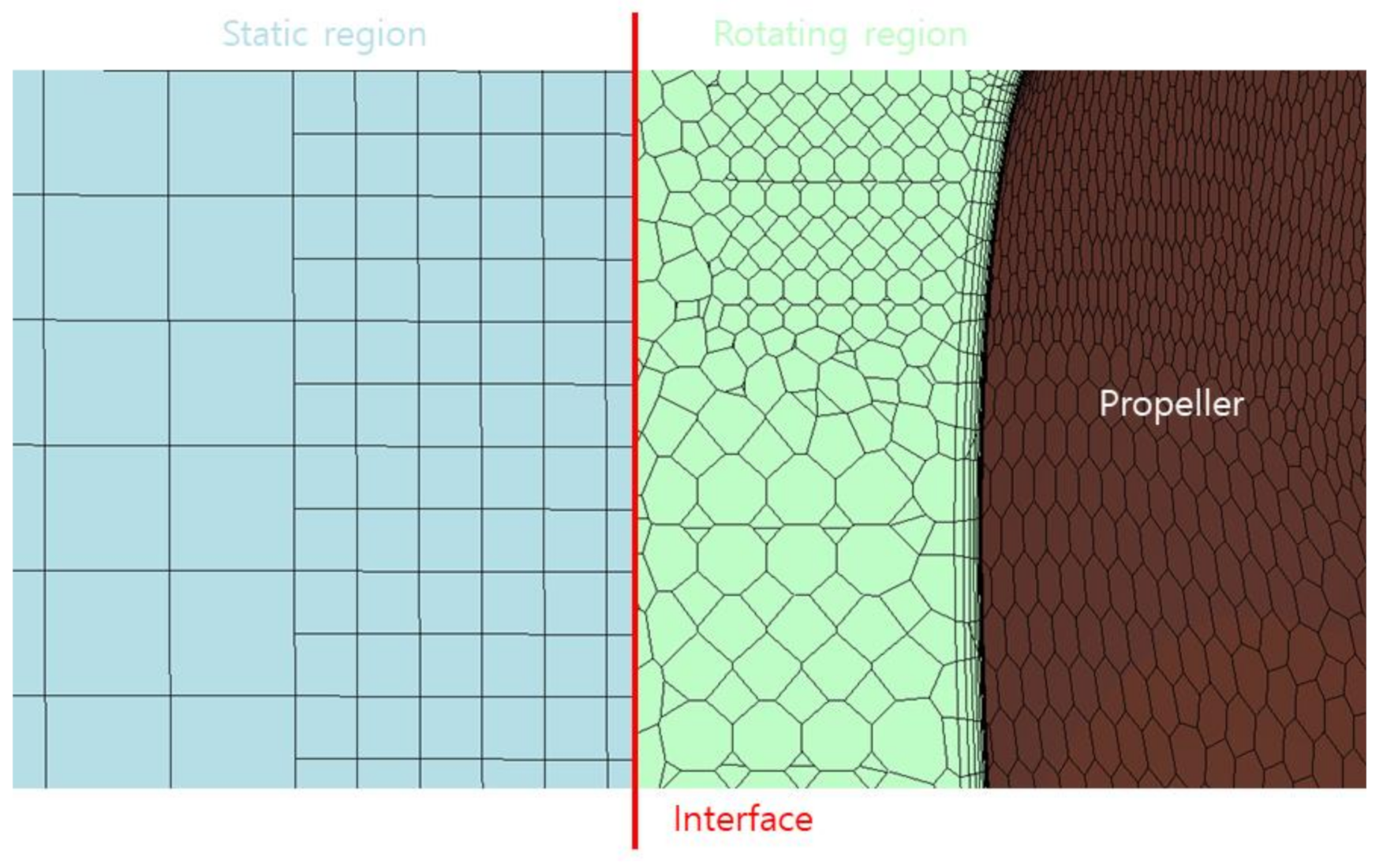
| Grid | Hexahedral | Hexahedral (static region) Polyhedral (rotating region) | |
| Configuration | Symbol (Unit) | Value |
|---|---|---|
| Scale ratio | λ | 32.6 |
| Length between perpendicular | Lpp (m) | 282.0 |
| Breadth | B (m) | 45.0 |
| Draft | T (m) | 18.3 |
Publisher’s Note: MDPI stays neutral with regard to jurisdictional claims in published maps and institutional affiliations. |
© 2021 by the authors. Licensee MDPI, Basel, Switzerland. This article is an open access article distributed under the terms and conditions of the Creative Commons Attribution (CC BY) license (https://creativecommons.org/licenses/by/4.0/).
Share and Cite
Kim, D.-H.; Park, J.-C.; Jeon, G.-M.; Shin, M.-S. CFD Simulation for Estimating Efficiency of PBCF Installed on a 176K Bulk Carrier under Both POW and Self-Propulsion Conditions. Processes 2021, 9, 1192. https://doi.org/10.3390/pr9071192
Kim D-H, Park J-C, Jeon G-M, Shin M-S. CFD Simulation for Estimating Efficiency of PBCF Installed on a 176K Bulk Carrier under Both POW and Self-Propulsion Conditions. Processes. 2021; 9(7):1192. https://doi.org/10.3390/pr9071192
Chicago/Turabian StyleKim, Dong-Hyun, Jong-Chun Park, Gyu-Mok Jeon, and Myung-Soo Shin. 2021. "CFD Simulation for Estimating Efficiency of PBCF Installed on a 176K Bulk Carrier under Both POW and Self-Propulsion Conditions" Processes 9, no. 7: 1192. https://doi.org/10.3390/pr9071192