Full-Field Comparison of MRV and CFD of Gas Flow through Regular Catalytic Monolithic Structures

Abstract

Understanding the influence of gas flow maldistribution in honeycombs can be beneficial for the process design in various technical applications. Although recent studies have investigated the effect of maldistribution by comparing the results of numerical simulations with experimental measurements, an exhaustive 3D full-field comparison is still lacking. Such full-field comparisons are required to identify and eliminate possible limitations of numerical and experimental tools. For that purpose, spatially resolved flow patterns were simulated by computational fluid dynamics (CFD) and measured experimentally by non-invasive NMR velocimetry (MRV). While the latter might suffer from a misinterpretation of artefacts, the reliability of CFD is linked to correctly chosen boundary conditions. Here, a full-field numerical and experimental analysis of the gas flow within catalytic honeycombs is presented. The velocity field of thermally polarized methane gas was measured in a regular 3D-printed honeycomb and a commercial monolith using an optimized MRV pulse sequence to enhance the obtained signal-to-noise ratio. A second pulse sequence was used to show local flow propagators along the axial and radial direction of the honeycomb to quantify the contribution of diffusion to mass transport. A quantitative comparison of the axially averaged convective flow as determined by MRV and CFD shows a very good matching with an agreement of ±5% and 10% for printed and commercial samples, respectively. The impact of maldistribution on the gas flow pattern can be observed in both simulation and experiments, confirming the existence of an entrance effect. Gas displacement measurements, however, revealed that diffusive interchannel transport can also contribute to maldistribution, as was shown for the commercial sample. The good agreement between the simulation and experiments underpins the reliability of both methods for studying gas hydrodynamics within opaque monolith structures.

1. Introduction

There is growing interest in the use of regularly and irregularly structured monoliths as catalyst supports or exhaust filters in chemical and automotive industries. These monoliths are often exposed to high gas throughput in the case of exhaust filters or to moderate gas flow rates in the case of catalyst supports in heterogeneously catalyzed reactions [1,2,3,4]. A large number of heterogeneously catalyzed reactions such as the methanation or hydrogenation of alkenes occur in the gas phase and overcoated monolithic catalysts such as open-cell foams and honeycomb structures. Thus, an accurate analysis, which considers the gas and solid phase separately, helps to understand the mass transport mechanism of gases throughout the monolithic supports in gaseous reactions. This can be used to reassess the theoretical assumptions that generally describe structured monoliths as an ideal network of square channels. Gulijk et al. [5] illustrated that the mass transport of gas is severely affected by minor geometrical alterations of the monolith channels. For instance, varying channel wall thicknesses, as well as cracked or skewed walls, cause a deviation from the ideal distribution of gas in a honeycomb monolith. This maldistribution was shown to have a considerable impact on the flow pattern, conversion, and temperature distribution in the monoliths [6].

The potential capability of nuclear magnetic resonance (NMR) for the investigation of the mass transport of gas in opaque systems has turned it into a powerful technique in engineering communities [7,8,9,10,11]. The reason for this is the possibility of a noninvasive analysis of the gas hydrodynamics, i.e., of velocity, diffusion, temperature, and concentration under experimental conditions. Newling [12] reviewed the efforts taken to measure gas flow by magnetic resonance velocimetry (MRV). Since then, excellent studies have been published on the mass transport of gas, particularly for monolithic structures [13,14,15,16]. The magnetic resonance imaging (MRI) of thermally polarized gases has always been a challenging issue because of the low signal-to-noise ratio (SNR) caused by low density, fast diffusivity, and short NMR relaxation times [7]. As solutions, either hyperpolarization techniques [11] have been applied or NMR-friendly gases with strong signals have been used. An example for an NMR-friendly gas is SF₆ due to its high MRI signal and its low diffusion coefficient compared to other thermally polarized gases [11,17,18,19]. For instance, Ramskill et al. [18] used SF₆ to investigate velocity fields in exhaust filters. More recently, Cooper et al. succeeded in obtaining velocity fields and the turbulent diffusivity of SF₆ gas in wall-flow channels by applying a compressed-sensing imaging technique [20]. However, one vital aspect of measuring thermally polarized gases instead of hyperpolarized gases is the possibility of investigating technically relevant species, such as methane gas for the methanation reaction. This allows the diffusivity and gas flow in monoliths to be obtained at relevant conditions. Despite the difficulties in the MRI of thermally polarized gases, there is still room to improve the SNR obtained in the MRI of gases. Recently, a straightforward technique for the full-field analysis of thermally polarized gases in porous media was proposed [21]. The method makes a trade-off between excitation angle, echo time $\left(TE\right)$, and repetition time $\left(TR\right)$ to improve the signal-to-noise ratio (SNR) of MRI images.

Computational fluid dynamics (CFD) simulations can be used as an alternative method to investigate the convective gas flow in monoliths. The effect of maldistribution, which is caused by the blockage of flow and, thus, the nonuniform distribution of flow, on the thermal and catalytic performance of monolithic structures has been investigated with the aid of numerical simulations for heat exchangers and automotive catalytic converters [22,23,24]. Agrawal et al. [6] studied a full-scale and reduced-scale geometry of a catalytic multi-channel monolith in the turbulent flow regime via two-dimensional CFD simulations. Due to the regular topology of the monolith, similar velocity profiles in both geometry scales were observed. In addition, the obtained velocity profiles showed the same trend for different flow rates within the monolith in both geometry scales. For irregular monolithic structures (such as open-cell foams) [25], the obtained velocity profiles at equal inlet velocities show differences between the full scale and reduced scale of the geometry. Choosing appropriate boundary conditions and utilizing identical structures in simulations and MRV measurements, however, led to good agreement between the simulation and experiments. Similar to regular monoliths, the same trends of velocity profiles for different inlet velocities were reported for irregular monoliths [25,26].

The results of the CFD simulation of flow within monoliths can be compared with experimental data in terms of conventional (integral) parameters such as the pressure drop along the structure [27]. Badami et al. [28] compared the CFD simulation results of the gas flow within the monolith exhaust systems in terms of velocity fields with the experimental results from hot-wire anemometry (HWA) measurements. Although the presented numerical and experimental velocity fields were reported to be in satisfactory agreement, the comparison was limited to only one axial position, which was 10 mm downstream of the catalyst. This limitation is due to the incapability of the HWA method to measure gas flow within opaque monoliths noninvasively. In another study, Tsinoglou et al. [29] compared the results of 2D CFD simulations and experimental measurements of the radial velocity profile at the entrance of a monolith. The HWA method cannot measure the effect of maldistribution on the flow patterns within opaque monoliths, and its capability is restricted to the measurement of velocity profiles at the entrance and exit of the monoliths. The method is thus not capable of a full-field comparison with CFD simulations.

Three-dimensional CFD simulations of gas flow within catalytic converters were reported to be extremely resource-intensive. Therefore, most CFD simulation studies used a 2D approximation of parallel channels to simulate 3D monoliths [6,22,24]. However, 3D CFD simulations were performed to analyze the flow distribution and individual contribution of each region on the total pressure drop in diesel particulate filters (DPFs), which have a more complex geometry compared to catalytic converters [30,31]. Cooper et al. [32] compared the results of 3D CFD simulations with 2D MRI velocity images of SF₆ gas flows within DPFs. Images were acquired perpendicular to the direction of flow at eleven axial positions, and axial velocity profiles in two inlet and outlet channels of the structure were compared with MRI measurements. The obtained isotropic spatial resolution of SF₆ was 140 µm per pixel.

Despite the fact that SF₆ provides a much better resolution compared to methane, we chose methane as the operating gas in this study as this system will be used for the methanation of CO₂ in our future studies. The choice of a thermally polarized gas for velocity measurements poses challenges in obtaining an appropriate SNR in MRI analysis. We use an optimized MRV pulse sequence that allows the enhancement of the SNR in the velocity measurements [25]. The optimized MRI method allows us to measure 3D velocity fields in printed honeycombs with sufficient spatial resolution to be compared with CFD simulations. In addition, we used a second pulse sequence [10,33] to show flow propagators along the axial and radial directions of the honeycomb locally to support the MRV results. The experimental methods offered in these measurements are complementary to study and quantify the gas mass transport in the honeycomb monoliths.

In the present study, we perform full-field MRV of thermally polarized methane gas flowing through two different honeycomb monoliths and compare the results to CFD simulations. To the best of our knowledge, only a few 3D CFD studies on the effect of flow maldistribution within the monolithic catalytic converters have been reported, and none of them have considered a full-field comparison of CFD results with a nonintrusive method under identical experimental conditions. Recently, we reported a full-field comparison of microcomputed tomography (µCT)-based 3D CFD simulations and MRV measurements of the gas flow within complex and opaque open-cell foams [25]. Such a comparison is, however, still missing for the monolithic catalytic converters. In fact, the cross-validation of 3D CFD simulations and full-field velocimetry measurements will enable us to identify the restrictions of numerical and experimental tools to precisely characterize the mass transport in the monolithic catalytic converters. It is worth mentioning that using identical structures in simulations and measurements helps us to better understand the effect of excluding diffusion in simulations. We can improve the quality of the agreement by considering diffusion in the further numerical simulations. We perform measurements for a commercial ceramic honeycomb and a 3D-printed structure with channel sizes of ~1 and 2.4 mm, respectively. The use of a 3D-printed structure helps to better understand the transport mechanism of gas because of its ideal geometry and large channel size compared to the commercial ceramic honeycomb. The measurement of the 3D-printed sample can reveal information that may not be obtained by measuring the commercial honeycomb. In other words, it is fair to assume that possible geometrical imperfections in the commercial honeycomb structure (e.g., cracks), the occurrence of bypass flow around the sample, or even MRV measurement errors may drastically affect the quality of the comparison between CFD and MRV. Hence, the 3D-printed structure was designed as a way to avoid the above-mentioned problems in the measurements. First, the 3D-printed geometry offers an ideal round shape to be perfectly fit into the setup, minimizing the potential bypass flow. Second, the channels of the 3D-printed geometry are free of cracks. Third, the larger channel size of the 3D-printed sample can be resolved more appropriately in the MRV measurements; thus, a lower contribution of measurement error is expected. In addition, the uncertainty of the MRV measurement is calculated based on the theoretical prediction and the obtained SNR in the experiments.

2. Materials and Method

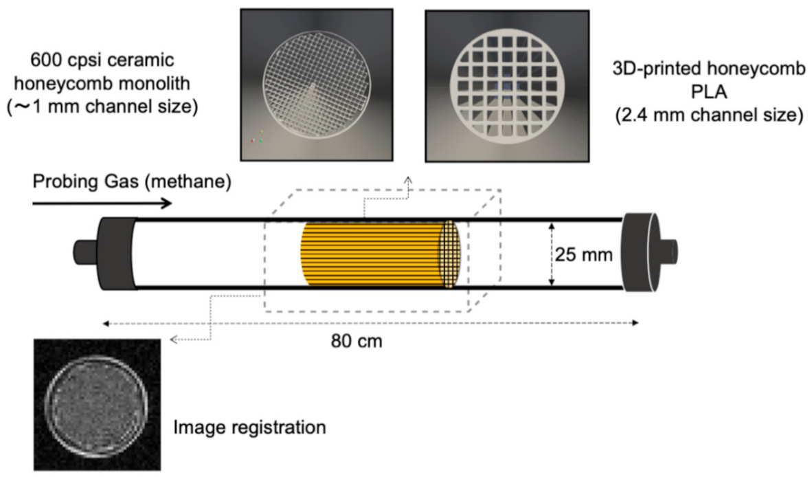
2.1. Experimental Setup

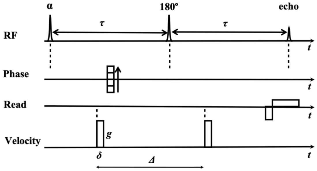
A glass vessel (ID: 25 mm, length: 80 cm) was used for the gas flow measurements. Two monoliths were used in the measurements, a commercial cordierite honeycomb monolith (length: 40 mm, diameter: 25 mm, 600 cells per square inch (cpsi), NGK, Poland) and a 3D-printed honeycomb made of PLA (polylactide). The latter offers a larger channel size as compared to the commercial cordierite honeycomb. To print the sample made of PLA (length: 40 mm, diameter: 25 mm, channel size: 2.4 mm), a 3D printer Ultimaker 3 (Ultimaker, Netherlands) with a nozzle diameter of 0.4 mm and resolution of 12.5 × 12.5 × 2.5 µm³ (layer height in vertical direction: 200 µm) was used. The sample was printed at an operating temperature of 215 °C. Both honeycombs were fitted into the cylindrical glass vessel separately using a sealing cord around the samples to prevent vibration of the sample during the measurements and to minimize bypass flow. However, the occurrence of a bypass flow for the commercial structure due to its nonideal wrapping seems to be inevitable. A methane flow was supplied into the cylindrical vessel through a mass flow controller (FMA-2618-A, Omega Engineering, Norwalk, CT, USA). Finally, the experimental setup illustrated in Figure 1 was inserted into the horizontal bore of a 7T superconducting magnet. The horizontal 7-Tesla MRI scanner (BioSpec 70/20 USR, Bruker BioSpin MRI, Ettlingen, Germany) was equipped with a 114 mm inner bore gradient system (B-GA 12S2) enabling a maximum gradient strength of 440 mT·m⁻¹ in each direction ($x,y,z$). All measurements were performed at ambient temperature and a pressure of 1.5 bar. Along the pulsed field gradient stimulated echo (PFG-STE) experiments with a volumetric flow rate of 1.5 SL min⁻¹, additional flow rates were applied (0.5, 1.0, and 2.0 SL min⁻¹) to determine the effect of flow on the displacement of gas in the radial and axial directions.

2.2. MRV Sequence

Flow velocity can be measured using phase-contrast MRI by applying velocity encoding gradients. The velocity of flow can be calculated by measuring phase differences during the signal encoding:

$$\phi -{\phi }_0=\gamma ·\nu · M_1.$$

(1)

Here, $\gamma$ is the gyromagnetic ratio and $\nu$ is the velocity. The parameter $M_1$ denotes the first moment of the gradient at echo time (TE) in a single direction. Therefore, only velocities along a single direction can be measured. To perform 3D velocimetry, however, a minimum of four encoding steps applied in positive and negative directions are necessary.

Here, a 3D MRI of the gas was conducted using a spin-echo-based phase contrast (SE PC) MRV sequence. A scheme of the implemented pulse sequence is given in Figure 2. Two phase encoding gradients were applied in the transversal direction ($x, y$) accompanied by a read gradient in the axial direction ($z$) to obtain a 3D spatial resolution. Three steps were taken to optimize velocity measurements of the methane gas in the porous structure: $TR$ and excitation flip angle adjustment; choice of $TE$ based on the transversal relaxation time ($T_2)$ and the diffusion coefficient $D_{\infty }$; and finally, the implementation of RF phase cycling to suppress unwanted signal contributions. Accordingly, the excitation angle was chosen based on the Ernst angle to increase the SNR [21]. A pair of unipolar velocity encoding gradients were applied prior to and after the refocusing pulse to determine velocity vectors in the regions of interest (ROI). The velocity encoding gradients also act as crusher gradients to suppress unwanted coherence pathways. The velocity encoding gradients were applied in four steps according to the Hadamard approach [34,35]. Using a field of view ($FOV$) of 96 × 64 × 64 mm³ and a matrix size of 120 × 80 × 80, the volume element (voxel) size was 0.8 × 0.8 × 0.8 mm³. The measurements were averaged 8 or 16 times to improve the SNR. Using a flip angle of 127°, a $TE$ of 3.15 ms, and a $TR$ of 50 ms, the total measurement time was about three hours if 8 averages were used.

A velocity encoding range [-VENC, +VENC] with $VENC$ = 300 mm$·$s⁻¹ was used according to the expected maximal velocity for flow rates of 1.5 SL min⁻¹. The flow encoding duration and flow encoding delay were ${}_{\mathrm{MRV}}$ = 0.37 ms and ${}_{\mathrm{MRV}}$ = 1.69 ms, respectively.

2.3. Error Estimation in MRV Measurements

MRV precision is denoted as the standard deviation (STD) of velocities in the region of the honeycomb. Theoretically, it could be estimated by an ideal model given by Pelc et al. [35]:

$$\sigma \left(v\right)=\frac{2 VENC}{\pi ·\mathrm{SNR}}.$$

(2)

In the present study, a SNR of ~14 was obtained for the 3D magnitude images measured with 8 averages. Here, the SNR was estimated by dividing the mean image intensity of methane-containing voxels in the reactor bore by the STD of image intensities of voxels outside the reactor bore. Then, the calculated STD was modified according to the Hadamard encoding approach for flow measurements, where the complex-valued image data are used to calculate changes in the signal phase due to flow. According to Equation (2) and with VENC = 300 mm·s⁻¹, the aforementioned SNR value results in a nominal σ of about 20 mm·s⁻¹. The STD of velocity decreases if more averaging is performed, e.g., 16 measurements. While choosing a high velocity encoding (VENC) value causes a higher STD of velocities, a phase wrap-around and, thus, systematic errors can be avoided for higher velocities that may occur in the channels in the structures.

For the MRV measurements in the 3D-printed honeycomb, the velocity-to-noise ratio (VNR) was estimated as the ratio of the average velocity (${\overline{V}}_{\mathrm{center} }$ = 147 mm·s⁻¹) and its STD in the central pixel of arbitrarily chosen honeycomb channels (${\mathsf{\sigma }}_{\mathrm{center} }= 9.35 \mathrm{mm}·{\mathrm{s}}^{-1}$) in the MRV measurements for the 3D-printed honeycomb, yielding ${\overline{V}}_{\mathrm{center} }$/${\mathsf{\sigma }}_{\mathrm{center} }$ ~15.7. The VNR was also calculated for a single voxel in which both the solid and gas phase were combined in a single volume element, i.e., close to the wall of channels. This is supposed to cause a lower SNR compared with the SNR of the central voxels because of a lower gas signal. The average velocity ${\overline{V}}_{\mathrm{wall}}~117$ mm·s⁻¹ and ${\mathsf{\sigma }}_{\mathrm{wall}}=14$ mm·s⁻¹ yield a VNR (${\overline{V}}_{\mathrm{wall} }$/${\mathsf{\sigma }}_{\mathrm{wall}}$) of 8.4 for these voxels. To analyze the reproducibility of the MRV, as well as the SNR and VNR, absolute differences between two or three repetitive scans were computed. Thus, the mean velocities in the $x$- and $y$- directions in both honeycomb channels and sidewall regions that are substantially under such a threshold were regarded as negligible, i.e., no net transversal flow was found in both regions.

2.4. NMR Displacement Measurements

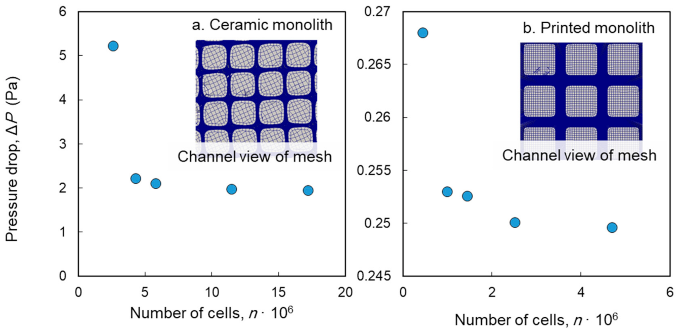
A Pulsed Field Gradient Stimulated Echo (PFG-STE) pulse sequence was used to measure the dispersion of gas in the radial and axial directions of the commercial honeycombs. The purpose of using the PFG measurements is to support MRV data in some cases. The PFG-STE enables measurements within a given volume element of the commercial honeycomb monolith. A scheme of the PFG sequence is available in the supplemental file provided in this work (Figure S1). Three 90° asymmetric pulses were implemented to restrict the measurements to a certain volume element of the monolith. In addition, a pair of diffusion-sensitized gradients were applied along the radial and axial directions to acquire the displacement function of gas in separate measurements. A detailed description of the PFG-STE can be found in our previously published articles [10,33].

Using the PFG-STE, we acquired the displacement functions of gas throughout the commercial honeycomb monolith in a volume of interest of 12 × 12 × 12 mm³. For all measurements, an observation time ${\mathsf{\Delta }}_{\mathrm{PFG}}$ = 10 ms, diffusion time ${\delta }_{\mathrm{PFG}}$ = 0.25 ms, and $TR$ = 250 ms was used. In addition, 64 equally distanced q-space values were applied to obtain the displacement function by Fourier transformation along q. In order to increase the SNR in the measurements, 32–64 averages were performed. The total measurement time for each experiment was around 8 min.

2.5. CFD Model

CFD simulations were carried out to determine velocity fields within the utilized structures. For this purpose, the finite volume-based CFD software OpenFOAM 4.1 was used to simulate the incompressible flow of methane (Mach number is lower than 0.2). The utilized governing steady-state equations of continuity and momentum for incompressible and Newtonian flow in this study are [36].

$$\nabla ·\mathit{u}=0,$$

(3)

$${\rho }_{\mathrm{f}}\left(\mathit{u}·\nabla \right)\mathit{u}-{\mu }_{\mathrm{f}}{\nabla }^2\mathit{u}=\nabla p.$$

(4)

Here, u indicates the velocity vector, ${\mu }_{\mathrm{f}}$ is the dynamic viscosity of fluid, and p is the pressure. The SIMPLE (Semi-Implicit Method for Pressure Linked Equations-Consistent) algorithm was applied for pressure–velocity coupling and the simpleFoam standard solver was utilized for running simulations. An absolute tolerance of 10⁻⁶ was prescribed for solving the system of equations [36,37].

The Reynolds number $Re$ of the flow based on the vessel diameter was sufficiently low ($Re=ud/\nu$ = 74.5, where $u$ is the average bulk velocity, $d$ the diameter of the vessel, and ν the dynamic viscosity of methane) to confirm that no turbulence or formation of eddies can occur, neither at the entrance nor at terminal regions of the sample [4,38]. Two monoliths with different morphologies were studied, a 3D-printed honeycomb and a commercial ceramic honeycomb. The latter was scanned by μCT imaging, and CFD simulations were run on the reconstructed structure. An in-house-developed μCT scanner at the tomography division of the Technical University of Dresden was used for the μCT imaging. The μCT images were prepared using molybdenum as a target material, an angular resolution of 0.25°, acceleration voltage of 90 kV, cathode current of 170 μA, and exposure time of 0.4 s. The μCT images were processed via image processing (ImageJ version 1.43, https://imagej.nih.gov/ij/) and CAD (MeshLab, http://www.meshlab.net/) software to generate the triangulated structure of the monolith as an STL file. The monolith was combined with the body of the reactor to generate a uniform object using another CAD software (Freecad, https://www.freecadweb.org/). Then, the geometry was imported into the meshing software to generate the computational network. The channel size and wall thickness of the commercial ceramic honeycomb were 0.84 and 0.16 mm, respectively. The 3D-printed honeycomb with a channel size and wall thickness of 2.4 and 0.8 mm, respectively, was designed in the CAD software and then printed. To generate the computational network, CfMesh was used, and meshes with 17.2 and 4.7 million cells were chosen for the commercial and printed structure, respectively. To verify that the results are independent of the grid resolution, we calculated the pressure drop along the monoliths with five different grids for each structure. The results of the grid independency tests are shown in Figure 3, which also contains channel views of the utilized meshes for each honeycomb.

3. Result and Discussion

We first compare MRV and CFD for the commercial honeycomb sample in Section 3.1. The commercial sample has such small channels that it is not possible to experimentally resolve them. As we experimentally found that velocity vectors are not straight (Section 3.1.1), we used the PFG-STE sequence to investigate radial and axial dispersion in the sample (Section 3.1.2). The PFG-STE complements the performed MRV measurements for the commercial honeycomb and helps to understand the interchannel displacement of the flowing gas. Next, we investigated the 3D-printed honeycomb. Due to the much larger channel diameters, we can fully resolve them experimentally, making comparisons with CFD easier. We compared both numerical and experimental velocity profiles (Section 3.2.1), as well as flow contraction and expansion (Section 3.2.2).

3.1. Commercial Honeycomb

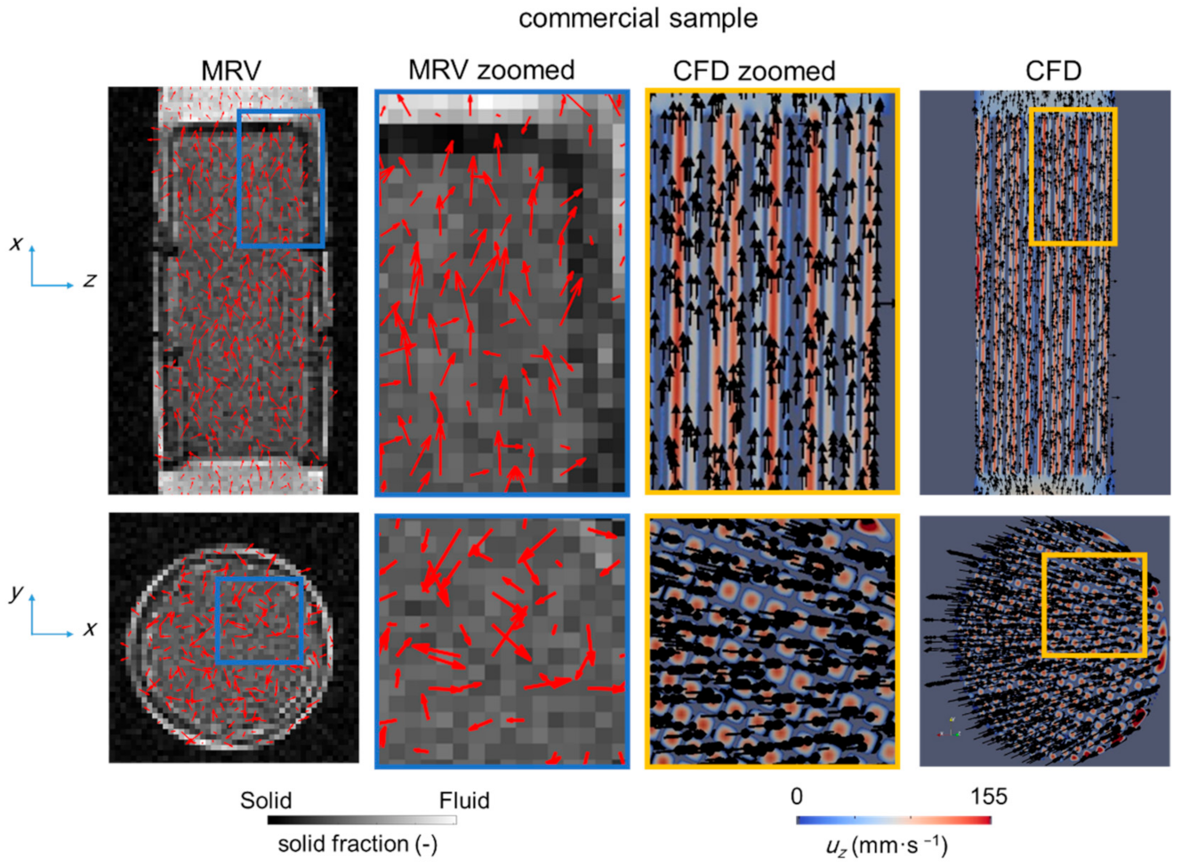
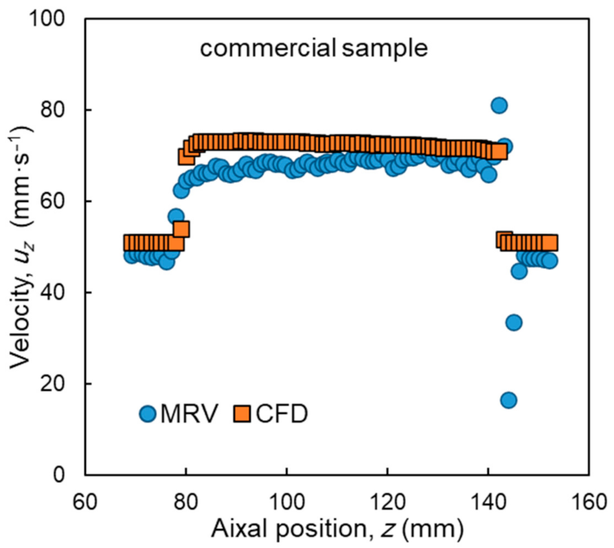
3.1.1. Comparison of Velocity Fields

The present study compares the full velocity fields between MRV and CFD data for identical structures. MRV measurements and CFD calculations of the velocity vectors in the commercial ceramic honeycomb are shown in Figure 4, which illustrates the $xz$- and $xy$-slices of the same plane in MRV and CFD data with overlaid velocity vector fields. While MRV fails at resolving the channel size of ~1 mm, in general, the velocity vectors lay in the positive axial direction. The vectors obtained in CFD data, by contrast, are entirely straight, and no drift or wave or zigzag motion can be observed in the channels, as expected. This is because the applied procedure for reconstructing CT images of the commercial ceramic monolith led to a smooth surface and therefore to uniform velocity profiles.

The averaged axial velocity profiles in the CFD simulations and MRV measurements at the flow rate 1.5 SL min⁻¹ are shown in Figure 5. The CFD and MRV results show a similar trend. The axial velocity increases as soon as the gas reaches the honeycomb structure and consequently remains at a constant range within the structure until it leaves the honeycomb.

The agreement between the obtained velocity profiles within the commercial ceramic monolith from CFD and MRV is ±10%, which is slightly less compared to the 3D-printed structure (see Section 3.2). This means that the measured averaged velocity profile in each axial position within the commercial sample did not exceed ±10% of the calculated value in Figure 5. Especially, there is a slight but systematical mismatch between the simulation and experiments in the first 20 mm of the monolith in Figure 5 (axial position of z = 80–100 mm). The mismatch is pointing toward an underrepresented velocity measurement that can be explained as follows:

First, the deviation between CFD and MRV can also partially be explained by the noise in the NMR data, especially at voxels containing both solid and gas (partial volume effect). In regions where the MRV data contain both the solid and gas phase, the SNR is reduced because of the lower obtained gas signal compared to pixels containing pure methane. This effect is pronounced for the data in the commercial structure as the channel size is extremely close to the MRV voxel size and the wall thickness is one-fifth of an MRV voxel size (as compared to the printed structure that has much larger channel sizes). Thus, pronounced deviations of velocity vectors between MRV and CFD are expected.

Second, the possible interchannel movement of gas in the radial direction can intensify the maldistribution of flow and thus increase the deviations between CFD and MRV results. We assume that gas can be transported through convection or diffusion through micro-cracks between walls of the monolith. These micro-pores and -cracks cannot be resolved via µCT images (with a voxel size of roughly 26 microns). Diffusion is also not considered in CFD simulations. Therefore, the effect of diffusion on such interchannel movement of gas cannot be shown by our simulations.

Third, there might be a bypass flow caused by a nonideal insertion of the sample, i.e., remaining voids between the wall and the monolith, which cause local changes in the porosity. Higher velocities were observed in some regions close to the wall, which suggest bypass flow occurrence (Figure 4). In contrast to the printed monolith, the utilized commercial ceramic monolith did not have a perfect circular cross-section, because of several defected channels in the wall region. These defected channels led to a flow bypass near the wall as the sample was not ideally fit to the wall of the vessel. In particular, the first half of the ceramic monolith had more defected channels that caused more deviation between the CFD and MRV results. These defected channels can be seen with the naked eye on the original monolith and are also observable in the reconstructed structure of the ceramic monolith from µCT images.

In order to support the second hypothesis, PFG-STE displacement measurements were performed that may confirm the existence of diffusional and interchannel motion of the gas molecules in the commercial honeycomb structure. These results are discussed in the next section.

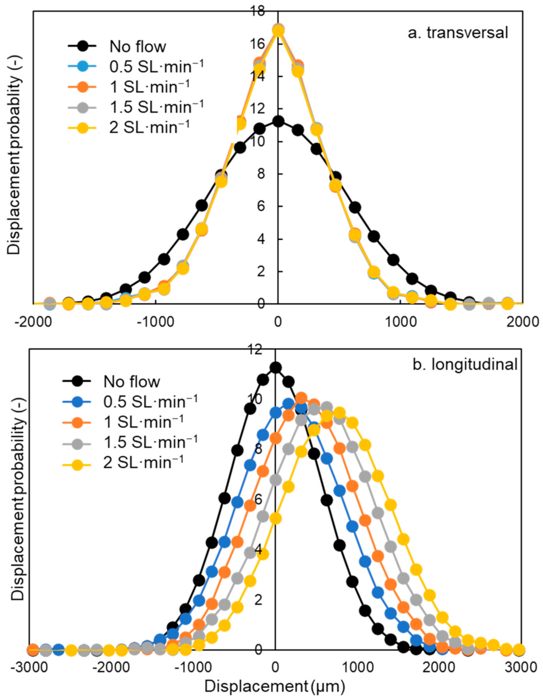
3.1.2. Radial and Axial Dispersion in Monolith Channels

According to the observations in Figure 4, it is difficult to merely relate the nonideal distribution of the velocity vectors in the commercial samples to the effect of walls on the gas flow. Thus, the potential interchannel movement of gas molecules in the radial direction of the commercial honeycomb was investigated using a spatially resolved PFG-STE sequence at an observation time of 10 ms and for various flow rates (0.5 to 2.0 SL·min⁻¹). The sequence offers a local resolution of 156 µm, turning it into an accurate method to investigate the gas displacement in the axial and radial direction. Figure 6 shows the gas displacement probability distributions (flow propagators) in transversal (radial) and longitudinal (axial) directions at various flow rates. The data points in the propagators are given in an equidistant displacement length of 156.25 µm. To better understand the probability distribution function, the maximum displacement length ($\mathsf{\Delta }{L}_{\max }$) was calculated from the tails of the propagators, where the functions approach the x-axis at both sides, indicating the maximal displacement length of the gas ensemble within the given observation time. The transversal gas propagators show a very similar probability distribution at different flow rates independent of the gas flow velocity, i.e., $\Delta L_{\max }$ is constant for all velocities (Figure 6a).

The gas propagators obtained at transversal flow are distinguishable from the propagator obtained for nonflowing gas (depicted by filled black markers) as they form propagators with higher stagnant peaks. This can be attributed to the increased collisions of the gas molecules with zero net displacement length in the channels along the transversal direction for a given observation time. The longitudinal propagator, however, depends on the flow rate as the maximum displacement $\mathsf{\Delta }{L}_{\max }$ increases with the flow rate (Figure 6b). In addition, increasing flow rates create propagators with positive (displacement) peaks toward the flow direction as the gas ensemble experiences a lower hindrance in axial direction compared to the radial direction.

Comparing the $\mathsf{\Delta }{L}_{\max }$ of the gas propagators in both radial and axial directions for a given flow rate (Figure 6a,b), the extent of hindrance in the radial direction caused by honeycomb channels can be observed. It is evident that the gas ensemble in the radial direction is restricted ~25% more as compared to its corresponding propagator in the axial direction.

From Figure 6b, the gas molecules’ maximal displacement length in the radial direction (~1.2 mm) is greater than the channel length size (~1 mm). This observation is similar to a former finding [10] that was explained by the migration of gas molecules from one channel to neighboring channels. This behavior of the flow is attributed to micro-cracks in the channel walls. One can also conclude from Figure 6a that the extent of radial displacement does not change with flow rates, as all the propagators are almost identical at various flow rates. The broader gas baseline and peak width of the propagator in the axial direction is attributed to the lower hindrance of gases in plug channels of the monolith.

The results in Figure 6b are superimposed with the propagator of self-diffusing methane gas as a reference to compare the displacement probability function of the gas. Additionally, dispersion coefficients were computed by relating the full-width at half-maximum ${\mathsf{\Delta }}_{1/2}$ to the observation time $\left({\mathsf{\Delta }}_{\mathrm{PFG}}-\frac{\delta }{3}\right)$ in each probability function:

$$D_{\mathrm{axial}/\mathrm{radial}}=\frac{{({\mathsf{\Delta }}_{1/2})}^2}{16 \log \left(2\right)\left({\mathsf{\Delta }}_{\mathrm{PFG}}-\delta /3\right))}.$$

(5)

The obtained axial and radial dispersion coefficients are given in

Table 1. The measured radial and axial displacement coefficients of flow within the ceramic monolith.

Flow Rate (SL·min−1)	$\mathbf{Radial} \mathbf{Dispersion} \mathbf{Coefficient} {\mathit{D}}_{\mathbf{radial}}\times {10}^{-6} ({\mathbf{m}}^2·\mathbf{s}{-}^1)$	$\mathbf{Axial} \mathbf{Dispersion} \mathbf{Coefficient}{\mathit{D}}_{\mathbf{axial}}\times {10}^{-5} ({\mathbf{m}}^2·\mathbf{s}{-}^1)$
0	11.2	1.62
0.5	6.79	2.14
1.0	6.78	2.12
1.5	6.82	2.23
2.0	6.70	2.37

. Without flow, the radial dispersion coefficient is about 30% lower than the axial dispersion coefficient, as the value of ${\mathsf{\Delta }}_{1/2}$ for the radial propagator is slightly lower. With flow, the dispersion coefficients in the radial direction are equal, whereas axial dispersion coefficients increase with the flow rate. A comparison of axial dispersion coefficients for a flowing gas ($6.7–6.82 \times {10}^{-6}$ m²·s⁻¹) against the diffusion coefficients without flow ($11.2 \times {10}^{-6}$ m²·s⁻¹) indicates a higher hindrance of flowing gas in the transversal direction. By contrast, axial dispersion coefficients increase for the flowing gas, indicating lower restrictions in the longitudinal direction.

We thus conclude that the interchannel transport of the gas, which is not resolved in the CFD simulation, influences the distribution of gas within the ceramic monolith and intensifies the maldistribution of the gas. In addition to the effect of the flow bypass described above, the interchannel displacement of the gas causes a reduction in the averaged axial velocity u_z and thus lowers the axially averaged velocity profile in the NMR measurements, which increases the deviation in the velocity vectors from a straight direction (Figure 4).

3.2. The 3D-Printed Honeycomb

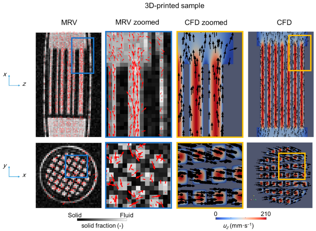
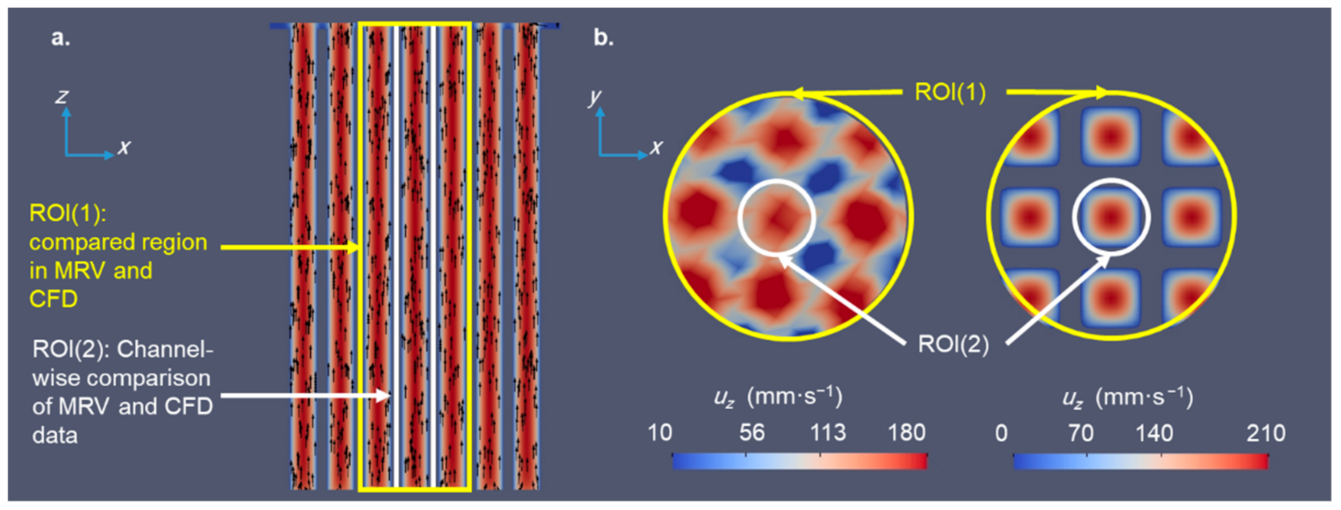
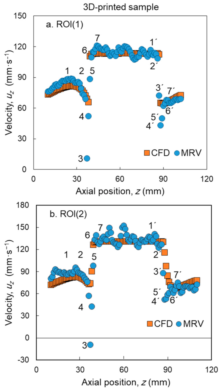
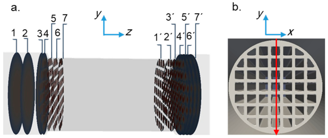
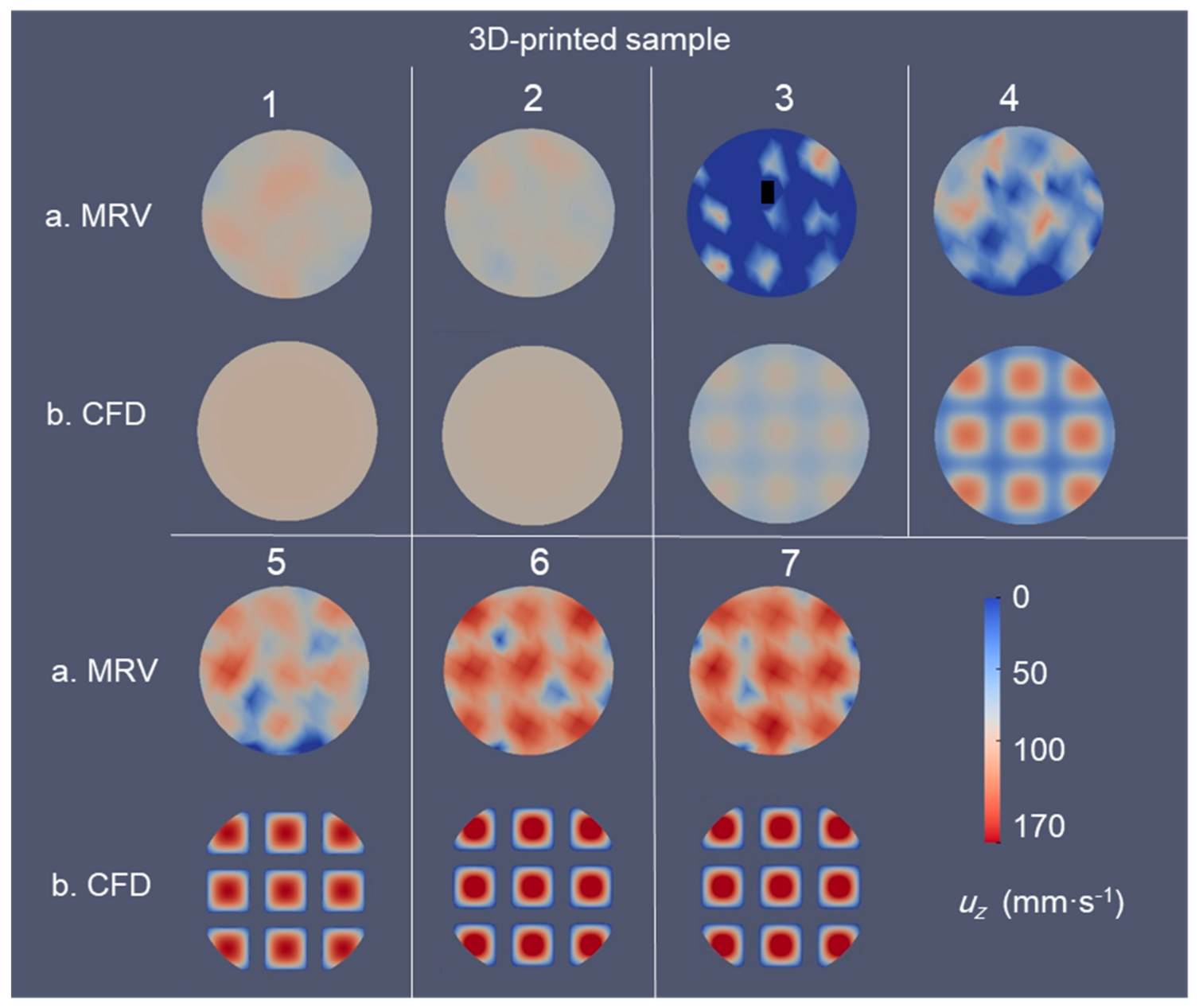
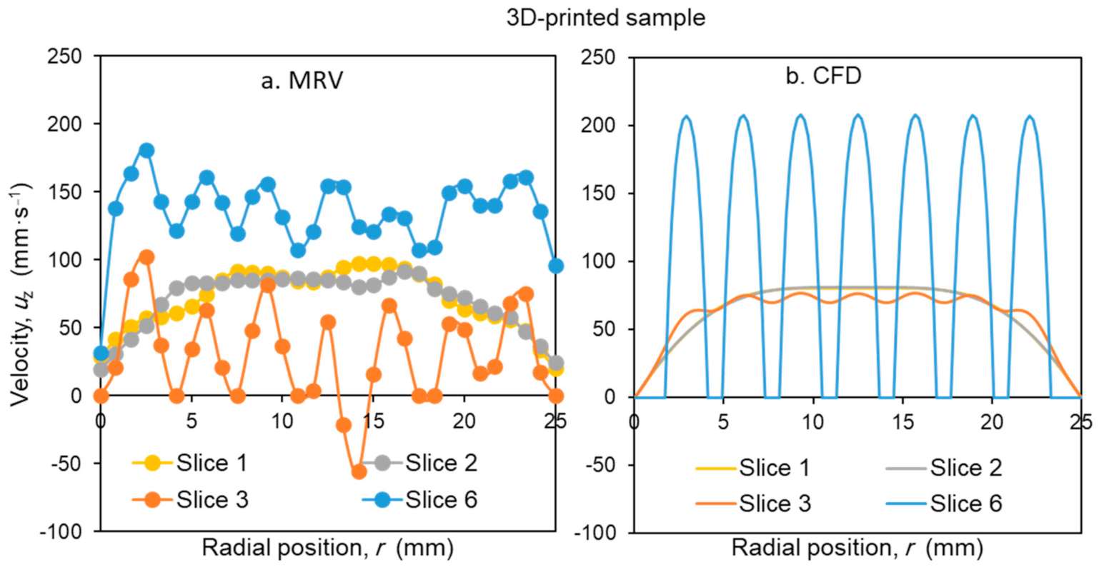
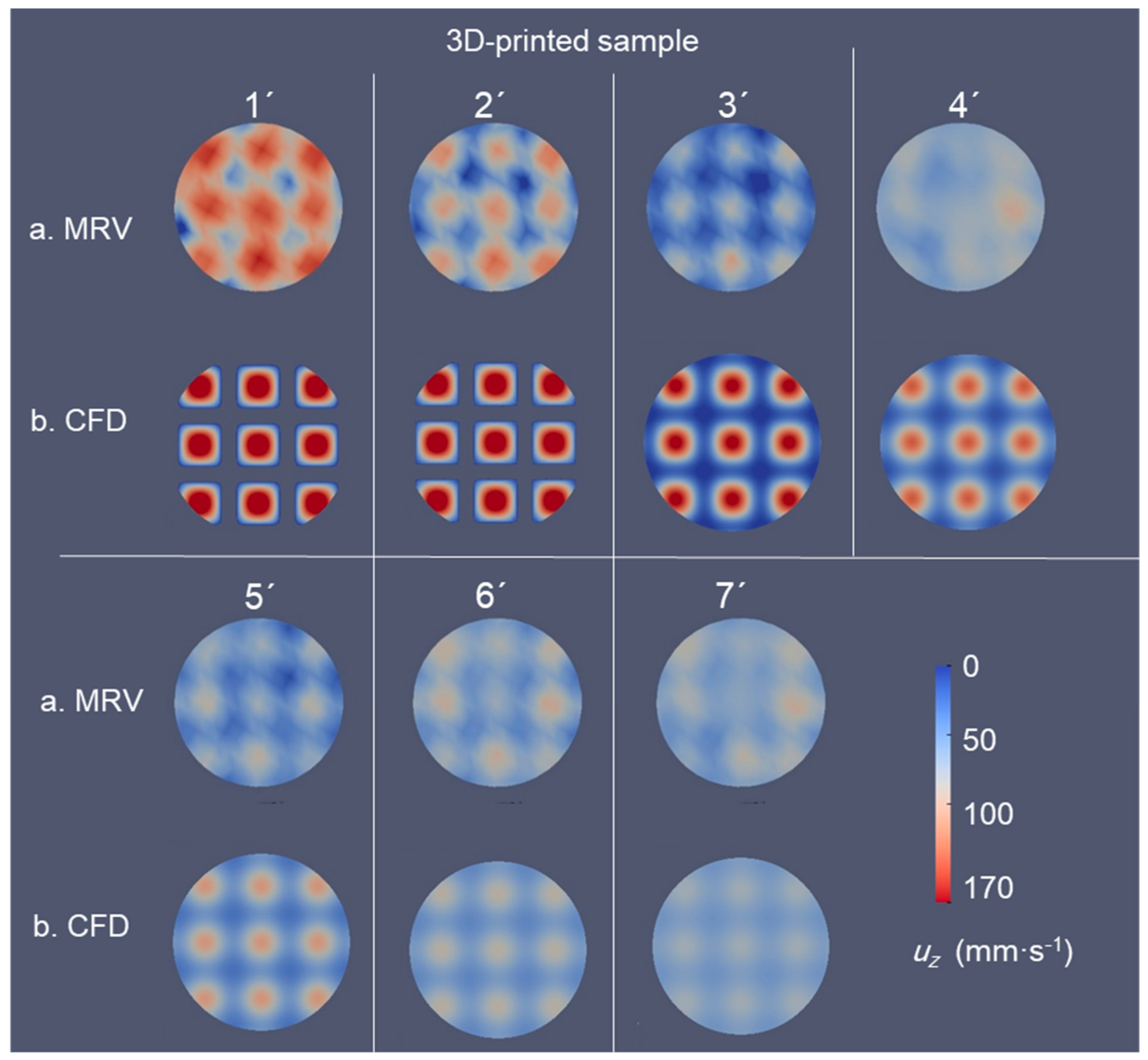
3.2.1. Comparison of Velocity Fields for 3D-Printed Honeycomb

As the MRV results do not resolve the channel of the commercial honeycomb sufficiently, a further comparison of CFD with MRV data of the commercial structure seems to be impractical. Therefore, the 3D-printed geometry with larger channels and wall thickness was chosen for further investigation. According to the resolution achieved in the MRV measurements and the channel size (2.4 mm, wall thickness 0.8 mm) of the 3D-printed honeycomb, each channel covers about nine pixels in MRV, allowing a detailed comparison of experimental data and simulations. Note that the CFD simulations were performed for an ideal honeycomb structure without µCT data for this comparison (cf. Figure 3). Therefore, the results of the simulations can be considered a pure theoretical prediction for the flow field. Considering the measurement error described in Section 3.1.2, deviations from the ideal velocity distribution in the axial direction in MRV data indicate gas–solid interactions within the monolith channels. Velocity vectors within commercial ceramic honeycombs obtained via both methods are shown in Figure 7. The majority of the MRV velocity vectors lay in straight, i.e., axial, directions in the $xz$-plane. However, the ridges and grooves in the channels from the layer-by-layer printing method of the 3D printer lead to differences in the surface roughness of the monolith channels and cause a maldistribution of the gas in the channels. In the CFD calculations, as expected, the velocity vectors in each monolith channel are all parallel and point in the axial direction. Compared to the commercial monolith with its smaller channel size, a better qualitative agreement can be observed between MRV and CFD results. Taking the predicted measurement error into account, the deviation of velocity vectors from a straight direction can be related to a lower SNR only to a certain degree, as described in Section 3.1.2, by determining VNR. In addition, the reproducibility of the measurements showed a similar trend of velocity vectors at arbitrarily chosen channel wall regions, confirming the impact of the ridges and grooves on the velocity vectors.

For a detailed comparison of the experimental and numerical results, two main regions of interests (ROI) were considered (cf. Figure 8). ROI(1) comprises the central area of a cross-section of the honeycomb with a diameter of 10 mm, including nine channels. ROI(2) instead comprises only the central channel of the monolith. The obtained averaged velocity profiles in the axial direction in the experiments and the simulations display a similar trend for both ROIs (cf. Figure 9). The comparison of gas flow rate within ROI(1) of the printed monolith obtained via CFD and MRV data is shown in Figure S2 in the supporting document. The flow calculated from the averaged velocity magnitude mostly agrees with a precision of ±5%. ROI(2) was taken to compare the velocities in a single channel as a representative volume of the 3D-printed honeycomb (Figure 9b). For both regions of interest and most values of z, the slice-averaged axial component of the velocity (u_z) calculated via CFD and measured via MRV are in good agreement. As problems such as the flow bypass, small cell size, and interchannel movement of gas caused by micro-cracks and diffusion are avoided by using a 3D-printed honeycomb, the quality of agreement is significantly improved compared to the results using the commercial monolith (cf. Figure 5). Due to the parabolic velocity profile before the monolith, the mean velocity in ROI(2) is higher as compared to ROI(1) (cf. Figure 9). Figure 9 also indicates that the velocity profile drops drastically in front of the entrance to the monolith and increases within the structure. This behavior can be described by the contraction of gas flow (caused by the decrease in flow cross-section) at the entrance region. After exiting the monolith, the velocity decreases instantly to a minimum value after which it increases smoothly in the hollow pipe. While the velocity profiles both at the entrance and the exit regions of the monolith show similar trends in MRV and CFD, a significant difference can be observed in both ROIs with respect to the minima shown by MRV data at points 3 and 4, as well as at 4′ and 5′. At these axial positions, the strong deviation is caused by some single pixels in the obtained MRV velocity fields. For example, the overall MRV velocity in slice 3 is negative, which is caused by two pixels having negative values of u_z. This can be attributed to MRV measurement errors where a significant reduction in the signal amplitude at the entrance region causes a large measurement error and, consequently, a deviation from the CFD data.

3.2.2. Upstream Flow and Downstream Flow

The flow contraction at the inlet region, also known as the entrance effect, causes a drop in pressure and affects the flow pattern, which contributes to the maldistribution of flow. The intensity of the contraction and its contribution to the total pressure drop depends on the type and geometry features of the monolith and the inlet velocity. The contribution of contraction to the total pressure drop in DPFs has been reported to be between 2 and 5%; the major part of the total pressure drop is caused by the porous wall between the inlet and outlet channels (66–73%) and the channel friction (19–20%) [39]. In contrast to DPFs, in straight-channel honeycombs, which we utilized in this study, a major pressure drop occurs within the channels, and the contraction of flow has a much lower contribution to the overall pressure drop (cf. Figure S3). In the present study, the pressure drop was computed by the CFD simulation within a channel in the flow direction, yielding a total of ∆P = 0.37 Pa. Within the honeycomb channels, the pressure drop follows a linear trend (Figure S3a) due to the regularity of the structure.

The averaged axial velocity reaches a minimum ahead of the honeycomb (Figure 9). This significant drop in velocity is caused by the contraction of gas flow in front of the honeycomb. The obtained velocity vectors from CFD and MRV also illustrate the compression of vectors toward the channels in front of the monolith honeycomb (Figure 7).

Velocity maps of cross-sectional MRI slices, corresponding to the axial positions given in Figure 10, are shown in Figure 11 and are compared with maps from CFD calculations. To better understand the flow pattern at the entrance region, the velocity field is shown at seven positions upstream of the monolith in Figure 11. The numbers of the shown slices correspond to the numbers in Figure 9a and Figure 10. While the flow is yet unaffected by the presence of the monolith honeycomb in slice 1, the contraction of flow in the entrance region is visible in slice numbers 3 and 4 with a sudden drop in velocity. Afterward, the velocity increases as the flow enters the monolith structure. The monolith contours are clearly observable in both MRV and CFD measurements. The average velocity reaches its maximum at slice number 7 after which it stays constant throughout the structure. The drop in the axial component of the velocity at the entrance region is more pronounced in MRV as compared to CFD data. This deviation can be seen in points 3 and 4 in Figure 9a quantitatively and in the corresponding slices 3 and 4 in Figure 11 qualitatively. The obtained velocity fields of slices 3 and 4 by MRV contain pixels with much lower values of velocities compared to the CFD ones. There are two pixels in slice 3 with negative values of the velocity, which contribute to the higher drop in the obtained velocity profile from MRV compared to the CFD profile.

The measured and simulated radial velocity profiles of u_z over an aligned arbitrary line (which is illustrated in Figure 10b) on the slices illustrated in Figure 10 (numbers 1–3 and 6) are shown in Figure 12. Similar velocity profiles for slice number 1 (yellow) and 2 (gray) were obtained from both MRV and CFD results. The measured and simulated velocity profiles of slice 3 (orange) show similar trends compared to slices 1 and 2. In contrast to other regions, the maxima and minima of u_z are more pronounced by MRV compared to CFD for slice 3. It can be concluded that at the entrance region, the contraction and maldistribution of flow were pronounced higher in MRV measurements. In addition, the velocity field in slice 3 shows the two pixels with negative values of u_z, which can be regarded as an MRV error. These two pixels are shown in slice 3 in Figure 11 by black squares. Velocity profiles in slice 4 (blue) show the same trend in MRV and CFD. Thus, apart from deviations in slice 3, through the rest of the monolith, the maxima and minima of the velocity are more pronounced in the simulation compared to the experimental data. This is expected as the resolution of MRV is lower than that from the CFD simulations. The MRV data thus contain pixels belonging to both the solid and fluid domain. This partial volume effect reduces the signal intensity in those pixels. Figure 12 compares the relative trends of the results from CFD and MRV. A direct comparison of CFD and MRV radial velocity profiles for each slice is shown in Figure S4. The measured velocity profiles in front of the monolith (Slices 1 and 2 in Figure S4a) are higher than the simulated ones. In the case of slice 3 (Figure S4b), the MRV velocity profile shows more fluctuations than the simulated profile. This is in line with the observation of a more intense entrance effect in MRV measurements. In addition, the first and last channels in slice 3 show higher velocities in the measurement. As discussed before, once in the monolith, extrema of the velocity are more pronounced in the CFD simulations than in MRV data. This can be seen by comparing the radial velocity profile of slice 6 in Figure S4b.

A corresponding behavior is observed at the exit region of the monolith, as can be seen from the velocity maps (Figure 13) and velocity profile (Figure 9). The flow drops from slice 2’ to 4’ and partially recovers from slice 5’ to 7’. The flow expands at the outlet over a longer distance compared to the entrance. In both MRV and CFD data, it was observed that the flow does not directly return to a laminar flow profile after flowing out of the structure [20]. The monolith structure is still visible in the surface plots of both MRV and CFD, i.e., the flow velocities in all slices (Figure 13). This corresponds to a maximum axial distance of 8 mm from the monolith exit.

4. Conclusions

The overview of the roadmap of this study is illustrated in Figure 14. The optimized phase-contrast MRI allowed a measurement of methane gas flow through the honeycombs with a sufficient SNR and spatial resolution. Using a full-field cross-validation of the CFD and MRV of flow within a 600 cpsi commercial monolith, we identified possible reasons for a deviation between simulations and experiments such as the radial interchannel flow caused by possible micro-cracks within walls, flow bypass, and the limited resolution of MRV velocity fields compared to the channel size (i.e., the channel size is in the range of the MRV voxel size). We thus used a 3D-printed monolith with a larger cell size and without structural imperfections to analyze mass transport in the absence of interchannel flow and flow bypass. In this case, the 3D CFD simulation of convective flow, which did not consider the diffusional transport of gas, and the MRV measurements showed better agreement. Additionally, a channel-wise analysis of flow velocity was carried out by comparing MRV and CFD. The comparison suggests that one cause of maldistribution in monoliths is the entrance effect. Figure 14 briefly illustrates the strategy of the paper for investigating the mass transport of gas in the honeycombs and the obtained agreement between CFD and NMR data. The MRV data can validate CFD models, while it gives an insight into the gas hydrodynamics in the monoliths. This introduces both methods as promising options for the full-field analysis of gaseous flow maldistribution within opaque monoliths. Furthermore, the gas displacement profiles obtained by volume-selective PFG-STE measurements showed interchannel transport for the commercial ceramic honeycomb monolith and revealed this to be the second possible cause for the maldistribution of flow. The NMR results emphasize the importance of considering diffusional transport in such systems for a more accurate prediction of gas behavior in gas–solid reactive systems at the entrance and exit region.

References

1. Eggenschwiler, P.D.; Tsinoglou, D.N.; Seyfert, J.; Bach, C.; Vogt, U.; Gorbar, M. Ceramic foam substrates for automotive catalyst applications: Fluid mechanic analysis. Exp. Fluids 2009, 47, 209–222. [Google Scholar] [CrossRef]
2. Donsì, F.; Cimino, S.; Di Benedetto, A.; Pirone, R.; Russo, G. The effect of support morphology on the reaction of oxidative dehydrogenation of ethane to ethylene at short contact times. Catal. Today 2005, 105, 551–559. [Google Scholar] [CrossRef]
3. Neumann, B.; Elkins, T.W.; Dreher, W.; Hagelin-Weaver, H.; Nino, J.C.; Bäumer, M. Enhanced catalytic methane coupling using novel ceramic foams with bimodal porosity. Catal. Sci. Technol. 2013, 3, 89–93. [Google Scholar] [CrossRef]
4. Lucci, F.; Della Torre, A.; Montenegro, G.; Dimopoulos Eggenschwiler, P. On the catalytic performance of open cell structures versus honeycombs. Chem. Eng. J. 2015, 264, 514–521. [Google Scholar] [CrossRef]
5. Van Gulijk, C.; Linders, M.J.G.; Valdés-Solís, T.; Kapteijn, F. Intrinsic channel maldistribution in monolithic catalyst support structures. Chem. Eng. J. 2005, 109, 89–96. [Google Scholar] [CrossRef]
6. Agrawal, G.; Kaisare, N.S.; Pushpavanam, S.; Ramanathan, K. Modeling the effect of flow mal-distribution on the performance of a catalytic converter. Chem. Eng. Sci. 2012, 71, 310–320. [Google Scholar] [CrossRef]
7. Gladden, L.F.; Sederman, A.J. Recent advances in flow MRI. J. Magn. Reson. 2013, 229, 2–11. [Google Scholar] [CrossRef]
8. Han, S.I.; Pierce, K.L.; Pines, A. NMR velocity mapping of gas flow around solid objects. Phys. Rev. E-Stat. Nonlinear Soft Matter Phys. 2006, 74, 016302. [Google Scholar] [CrossRef] [Green Version]
9. Harel, E.; Granwehr, J.; Seeley, J.A.; Pines, A. Multiphase imaging of gas flow in a nanoporous material using remote-detection NMR. Nat. Mater. 2006, 5, 321–327. [Google Scholar] [CrossRef] [Green Version]
10. Mirdrikvand, M.; Ilsemann, J.; Thöming, J.; Dreher, W. Spatially Resolved Characterization of the Gas Propagator in Monolithic Structured Catalysts Using NMR Diffusiometry. Chem. Eng. Technol. 2018, 41, 1871–1880. [Google Scholar] [CrossRef]
11. Kovtunov, K.V.; Lebedev, D.; Svyatova, A.; Pokochueva, E.V.; Prosvirin, I.P.; Gerasimov, E.Y.; Bukhtiyarov, V.I.; Müller, C.R.; Fedorov, A.; Koptyug, I.V. Robust In Situ Magnetic Resonance Imaging of Heterogeneous Catalytic Hydrogenation with and without Hyperpolarization. ChemCatChem 2019, 11, 969–973. [Google Scholar] [CrossRef]
12. Newling, B. Gas flow measurements by NMR. Prog. Nucl. Magn. Reson. Spectrosc. 2008, 52, 31–48. [Google Scholar] [CrossRef]
13. Bouchard, L.-S.; Burt, S.R.; Anwar, M.S.; Kovtunov, K.V.; Koptyug, I.V.; Pines, A. NMR Imaging of Catalytic Hydrogenation in Microreactors with the Use of para-Hydrogen. Science 2008, 319, 442–445. [Google Scholar] [CrossRef] [Green Version]
14. Koptyug, I.; Altobelli, S.; Fukushima, E.; Matveev, A.; Sagdeev, R. Thermally Polarized (1)H NMR Microimaging Studies of Liquid and Gas Flow in Monolithic Catalysts. J. Magn. Reson. 2000, 147, 36–42. [Google Scholar] [CrossRef] [PubMed]
15. Koptyug, I.V.; Ilyina, L.Y.; Matveev, A.V.; Sagdeev, R.Z.; Parmon, V.N.; Altobelli, S.A. Liquid and gas flow and related phenomena in monolithic catalysts studied by 1H NMR microimaging. Catal. Today 2001, 69, 385–392. [Google Scholar] [CrossRef]
16. Gladden, L.F.; Mitchell, J. Measuring adsorption, diffusion and flow in chemical engineering: Applications of magnetic resonance to porous media. New J. Phys. 2011, 13, 035001. [Google Scholar] [CrossRef]
17. Sankey, M.H.; Holland, D.J.; Sederman, A.J.; Gladden, L.F. Magnetic resonance velocity imaging of liquid and gas two-phase flow in packed beds. J. Magn. Reson. 2009, 196, 142–148. [Google Scholar] [CrossRef] [PubMed]
18. Ramskill, N.P.; York, A.P.E.; Sederman, A.J.; Gladden, L.F. Magnetic resonance velocity imaging of gas flow in a diesel particulate filter. Chem. Eng. Sci. 2017, 158, 490–499. [Google Scholar] [CrossRef]
19. Ramskill, N.P.; Gladden, L.F.; York, A.P.E.; Sederman, A.J.; Mitchell, J.; Hardstone, K.A. Understanding the operation and preparation of diesel particulate filters using a multi-faceted nuclear magnetic resonance approach. Catal. Today 2013, 216, 104–110. [Google Scholar] [CrossRef]
20. Cooper, J.D.; York, A.P.E.; Sederman, A.J.; Gladden, L.F. Measuring velocity and turbulent diffusivity in wall-flow filters using compressed sensing magnetic resonance. Chem. Eng. J. 2019, 119690. [Google Scholar] [CrossRef] [Green Version]
21. Huang, H.L. Methods for Characterization of Mass Transport in Porous Materials. Ph.D. Thesis, Universität Bremen, Bremen, Germany, 2017. [Google Scholar]
22. Benjamin, S.F.; Haimad, N.; Roberts, C.A.; Wollin, J. Modelling the Flow distribution through automotive catalytic converters. Proc. Inst. Mech. Eng. Part C 2015, 215, 379–383. [Google Scholar] [CrossRef]
23. Zhang, L. International Journal of Heat and Mass Transfer Flow maldistribution and thermal performance deterioration in a cross-flow air to air heat exchanger with plate-fin cores. Int. J. Heat Mass Transf. 2009, 52, 4500–4509. [Google Scholar] [CrossRef]
24. Liu, Z.; Benjamin, S.F.; Roberts, C.A. Pulsating Flow Maldistribution within an Axisymmetric Catalytic Converter-Flow Rig Experiment and Transient CFD Simulation. 2003-01-3070. SAE Tech. Paper 2003. [Google Scholar] [CrossRef]
25. Sadeghi, M.; Mirdrikvand, M.; Pesch, G.R.; Dreher, W.; Thöming, J. Full-field analysis of gas flow within open-cell foams: Comparison of micro-computed tomography-based CFD simulations with experimental magnetic resonance flow mapping data. Exp. Fluids 2020, 61, 1–16. [Google Scholar] [CrossRef]
26. Onstad, A.J.; Elkins, C.J.; Medina, F.; Wicker, R.B.; Eaton, J.K. Full-field measurements of flow through a scaled metal foam replica. Exp. Fluids 2011, 50, 1571–1585. [Google Scholar] [CrossRef]
27. Kovacev, N.; Li, S.; Zeraati-rezaei, S.; Hemida, H.; Tsolakis, A.; Essa, K. Effects of the internal structures of monolith ceramic substrates on thermal and hydraulic properties: Additive manufacturing, numerical modelling and experimental testing. Int. J. Adv. Manuf. Technol. 2020, 112, 1115–1132. [Google Scholar] [CrossRef]
28. Badami, M.; Millo, F.; Zuarini, A.; Gambarotto, M. CFD Analysis and Experimental Validation of the Inlet Flow Distribution in Close Coupled Catalytic Converters. SAE Powertrain Fluid Syst. Conf. Exhib. 2003, 14. [Google Scholar] [CrossRef]
29. Tsinoglou, D.N.; Koltsakis, G.C. Transient modelling of flow distribution in automotive catalytic converters. Appl. Math. Model. 2004, 28, 775–794. [Google Scholar] [CrossRef]
30. Konstandopoulos, A.G. Inertial Contributions to the Pressure Drop of Diesel Particulate Filters Reprinted from: Diesel Exhaust Emission Control: Diesel Particulate Filters. 2001-01-0909. SAE Tech. Paper 2001. [Google Scholar] [CrossRef]
31. Liu, Z.G.; Miller, R.K.; Nelson, F.; Company, A.C. Flow Distributions and Pressure Drops of Wall-Flow Diesel Particulate Filters 2002-01-1311. SAE Tech. Paper 2002. [Google Scholar] [CrossRef]
32. Cooper, J.D.; Liu, L.; Ramskill, N.P.; Watling, T.C.; York, A.P.E.; Stitt, E.H.; Sederman, A.J.; Gladden, L.F. Numerical and experimental studies of gas flow in a particulate filter. Chem. Eng. Sci. 2019, 209, 115179. [Google Scholar] [CrossRef]
33. Mirdrikvand, M.; Sadeghi, M.; Karim, M.N.; Thöming, J.; Dreher, W. Pore-scale analysis of axial and radial dispersion coeffi cients of gas fl ow in macroporous foam monoliths using NMR-based displacement measurements. Chem. Eng. J. 2020, 388, 124234. [Google Scholar] [CrossRef]
34. Dumoulin, C.L.; Souza, S.P.; Darrow, R.D.; Pelc, N.J.; Adams, W.J.; Ash, S.A. Simultaneous acquisition of phase-contrast angiograms and stationary-tissue images with Hadamard encoding of flow-induced phase shifts. J. Magn. Reson. Imaging 1991, 1, 399–404. [Google Scholar] [CrossRef] [PubMed]
35. Pelc, N.J.; Bernstein, M.A.; Shimakawa, A.; Glover, G.H. Encoding strategies for three-direction phase-contrast MR imaging of flow. J. Magn. Reson. Imaging 1991, 1, 405–413. [Google Scholar] [CrossRef]
36. Versteeg, H.; Malalasekera, W. An Introduction to Computational Fluid Dynamics: The Finite Volume Method; Pearson Education: London, UK, 2007. [Google Scholar]
37. Report, T.; Pozzobon, V.; Centrale, E.; Lagragian, M.; View, O.T.; Pozzobon, V. OpenFOAM Advanced Tutorial. 2016. Available online: https://cfd.direct/openfoam/user-guide-v4/ (accessed on 14 February 2019).
38. Della Torre, A.; Montenegro, G.; Tabor, G.R.; Wears, M.L. CFD characterization of flow regimes inside open-cell foam substrates. Int. J. Heat Fluid Flow 2014, 50, 72–82. [Google Scholar] [CrossRef] [Green Version]
39. Masoudi, M. Hydrodynamics of diesel particulate filters. SAE Tech. Pap. 2002. [Google Scholar] [CrossRef]
Figure 1. The experimental setup used for gas flow measurements in the 600 cpsi and 3D-printed honeycomb samples. The results of magnetic resonance velocimetry (MRV) and computational fluid dynamics (CFD) were compared by performing image registration for both data sets. The MRV image shows methane (bright pixels) in the commercial honeycomb. The bright ring shows the bulk of methane in the sealing cord around the sample used to fit the honeycomb in the vessel.
Processes 09 00566 g001
Figure 2. Implemented single-SE PC MRV pulse sequence for 3D MRV of methane in the monoliths (not to scale). For slice-selective 2D imaging, soft RF pulses with slice-selection and slice-rephasing gradients in the slice direction are used instead of rectangular RF pulses, and phase encoding is only performed in one direction.
Processes 09 00566 g002
Figure 3. The grid independency test results for (a) ceramic and (b) printed monolith honeycombs. Both panels contain an inset showing a channel view of the final mesh.
Processes 09 00566 g003
Figure 4. The obtained velocity vectors for the flow rate of 1.5 SL min−1 of methane within the commercial monolith from MRV measurements and CFD simulations.
Processes 09 00566 g004
Figure 5. The radially averaged axial velocity uz in CFD simulations and MRV measurements for the flow rate 1.5 SL·min−1 within the commercial ceramic honeycomb.
Processes 09 00566 g005
Figure 6. Transversal (a) and longitudinal (b) gas propagator in the commercial monolith channels.
Processes 09 00566 g006
Figure 7. The obtained velocity vectors for the flow rate of 1.5 SL·min−1 of methane within the 3D-printed monolith from MRV measurements and CFD simulations.
Processes 09 00566 g007
Figure 8. (a) The chosen regions of interest (ROIs) selected to compare MRV and CFD data. (b) z -component of velocity in a central slice (ROI(1)) in experimental and numerical data. The depicted ROI for MRV data is tilted away from the CFD data by some degrees. As the comparison of velocity in ROIs was conducted based on the averaged velocity profile over the cross-sections, the rotated channels do not affect the comparison.
Processes 09 00566 g008
Figure 9. Comparison of the radially averaged axial velocity component obtained by CFD and MRV in (a) ROI(1) and (b) ROI(2). The axial position on the z -axis covers the entrance (1–7), inside (7–1′), and exit region (1′–7′) of the 3D-printed structure.
Processes 09 00566 g009
Figure 10. (a) The axial position of the investigated slices analyzed for upstream and downstream flow. (b) The arbitrary line over the cross-sectional slices used for plotting radial velocity profiles in Figure 12.
Processes 09 00566 g010
Figure 11. Axial velocity distribution along the entrance region within ROI(1) determined by MRV. The slice numbers correspond to the illustrated markers at the entrance region in Figure 9a. The two mentioned pixels at slice 3 with a negative value of uz are shown by black squares.
Processes 09 00566 g011
Figure 12. The velocity profile of uz over an arbitrary line (Figure 10) across the radius of the monolith determined by MRV (a) and CFD (b). Slices 1 to 3 and 6 correspond to the sample slice numbers given in Figure 6 and Figure 9. The yellow and gray curves show the bulk flow approaching the honeycomb. The orange curves show the flow at the interface of the flow and solid structure, where the contraction takes place. The blue curves represent the velocity profile in the monolith channels.
Processes 09 00566 g012
Figure 13. Axial velocity distribution along the exit region within ROI(1) as determined by MRV. The slice numbers correspond to the illustrated markers at the entrance region in Figure 8a.
Processes 09 00566 g013
Figure 14. The overview of the conducted study for the analysis of gas flow within the honeycomb monoliths.
Processes 09 00566 g014