CFD Modelling of a Hydrogen/Air PEM Fuel Cell with a Serpentine Gas Distributor

Abstract

Hydrogen-fueled fuel cells are considered one of the key strategies to tackle the achievement of fully-sustainable mobility. The transportation sector is paying significant attention to the development and industrialization of proton exchange membrane fuel cells (PEMFC) to be introduced alongside batteries, reaching the goal of complete de-carbonization. In this paper a multi-phase, multi-component, and non-isothermal 3D-CFD model is presented to simulate the fluid, heat, and charge transport processes developing inside a hydrogen/air PEMFC with a serpentine-type gas distributor. Model results are compared against experimental data in terms of polarization and power density curves, including an improved formulation of exchange current density at the cathode catalyst layer, improving the simulation results’ accuracy in the activation-dominated region. Then, 3D-CFD fields of reactants’ delivery to the active electrochemical surface, reaction rates, temperature distributions, and liquid water formation are analyzed, and critical aspects of the current design are commented, i.e., the inhomogeneous use of the active surface for reactions, limiting the produced current and inducing gradients in thermal and reaction rate distribution. The study shows how a complete multi-dimensional framework for physical and chemical processes of PEMFC can be used to understand limiting processes and to guide future development.

1. Introduction

The modern scenario for the automotive transportation sector is seeing more and more stringent emission regulations for traditional internal combustion engine vehicles (ICEV), relevantly increasing the powertrain cost due both to the complexity of the after-treatment devices (particulate filter, catalytic reduction systems, etc.) and/or by the coupling with an electric motor for hybrid powertrains. The interest towards carbon-free solutions for mobility is the motivation for a renewed attention on the possible uses of hydrogen as an energetic vector. It can be used either as a combustible fuel for ICEV or to produce electricity in proton exchange membrane fuel cells (PEMFC): While in the former strategy the peak formation of harmful nitrous oxide (NO_x) emerges as the most relevant obstacle, in the latter one water and low-temperature heat are the only by-products of on-board electricity generation, thanks to the absence of a thermal/combustion cycle. Despite the very high gravimetric energy content of hydrogen (with lower heating value of approx. 120 MJ/kg), its reduced density leads to very poor volumetric energy content. However, this poses the severe technological challenge of hydrogen storage to both strategies, for which highly-pressurized gas tanks (350 bar and 700 bar) are emerging as a de facto standard for several market-ready applications. This is a key milestone to de-carbonize transportation sectors for which a battery-based propulsion system is not a viable option (e.g., heavy-duty, off-highway, maritime, aerial), and it will play a crucial role in conjunction with the progress in other energy conversion systems [1,2,3,4] and simulation techniques [5,6].

Among the multiple types of fuel cells, PEMFC are receiving significant research and investment attention for the use in the transportation sector, mainly because of their low-temperature operation (in the range 340 K–380 K), good suitability for frequent start-stop cycles, and for the absence of corrosive substances (e.g., liquid acid). Their core component is a solid polymeric membrane impermeable to fluids, able to separate the hydrogen oxidation reaction (HOR, at the anode) and the oxygen reduction reaction (ORR, at the cathode). The most widespread polymer for PEMFC membranes is called Nafion, presenting a high proton conductivity, while platinum is typically used as a catalyst material deposited on carbon-based catalyst layers (CLs) on the two sides of the membrane.

Despite PEMFC being a well-established type of fuel cell, the complex interplay of physical and chemical processes that are key to a highly-efficient operation are still not fully understood, as is the role of materials on the overall cell performance. To fulfill this knowledge gap, computational fluid dynamics (CFD) modelling allows the numerical simulation of all the fluid/heat/charge transport phenomena, offering the incomparable possibility to identify limiting processes and driving the design and development of high-efficiency PEMFC. In recent years, a large body of literature on CFD modelling of PEMFC has been proposed, although there is still a need for considerable development in this field to obtain models with a high degree of accuracy, reliability, and applicability to industrial fuel cell design, as pointed out in Wang’s analysis [7]. Among the pioneering models proposed in the literature the 1D models by Springer et al. [8] and Bernardi et al. [9] paved the way for membrane models including a detailed water uptake curve. Moving to 3D models, a fundamental aspect in the PEMFC modelling is the grid resolution, especially in the through-plane (i.e., along the cell thickness) direction where despite the highest gradients develop (e.g., concentration of species, thermal and electrical fields) in small length scales (typically 10–1000 μm). Kamarajugadda and Mazumder [10] carried out a comparison on the accuracy and efficiency of the different membrane modelling strategies. The critical balance between diffusion and convection-dominated transport was investigated by Feser et al. [11] using a non-dimensional analysis and quantified by Pharoah [12] in a serpentine-sample with GDL of various permeabilities. Zeng et al. [13] proposed a non-dimensional Forchheimer number to characterize the flow regime in porous materials, and Zhang et al. [14] and Um et al. [15] showed the potential advantage of interdigitated designs. Choopanya and Yang [16] emphasized that the reactants’ diffusion in the gas diffusion layers (GDL), the transport of ions through the electrolyte membrane, and electronic transport in the conductive components mainly occur along the cell thickness, for which the lowest conductivity/permeability values are measured, thus constituting high-resistance transport pathways. Numerical analyses of the impact of the GDL parameters on flow transport are reported in Carcadea et al. [17]. As for the gas channel size/shape, in [18] the advantage of narrow channel/ribs on the uniform catalyst layer use was tested and simulated, and in [19] an analysis of the serpentine channel size and shape was conducted, including the discussion of the weight of advective/diffusive processes. Moving to CL modelling, a thin-layer approach was used by Berning et al. [20] was introduced to bundle the ultra-thin reacting layer into an interfacial reaction model, and a similar approach was followed by Zhang et al. [21] and Ferreira et al. [22]. Further insights regarding modelling techniques suited to reproduce all the types of transport processes in PEMFC are surveyed by Kulikoswky [23], Jiao et al. [24], Wu et al. [25], and Djilali [26].

In this study, an industrial-like hydrogen/air PEMFC with serpentine-type gas distributors also studied in [22] is used for the validation of a comprehensive multi-dimensional CFD model. In the next sections the details of the model governing equations first presented in [27,28] are further developed and they will be presented for the fluid/solid domains. The analyzed case will then be presented, and the results will be analyzed both in terms of characteristic curves (polarization and power density) and regarding the fields of the reactants’ concentrations, reaction rates, and thermal and liquid water distributions. Finally, an improved formulation of the cathodic exchange current density will be implemented, and conclusive guidelines on comprehensive 3D-CFD models will be provided.

2. Numerical Model

In this study a multi-phase/multi-physics modelling approach [7] is adopted to consider the presence of multiple phase fluids (e.g., liquid/vapor) in a PEM fuel cell, as well as of multiple components (fluid and solid). This introduces modelling challenges, due to concurring physical and electrochemical processes (fluid, heat, and charge transport) and phase change. Such processes are simulated by solving conservation equations for mass, momentum, energy, chemical species, and electric charges (electrons and protons). The presence of porous media imposes a dedicated flow treatment, as the modelling of reactants transport and of products removal through the gas diffusion layers is crucial for an optimal cell performance. Furthermore, a multi-phase fluid treatment is necessary due to the possible presence of condensed liquid water at the cathode at the low pressure and temperature conditions of interest. Finally, an important role is played by the characterization of the electrolyte material, impermeable to fluids but which allows the transport of ions and of dragged water within the solid polymer material. The following sections present the equations of the model for fluid (including the presence of porous regions) and solids. With reference to a preliminary model validation in [28], the 3D-CFD model is extensively developed here including the solid bi-polar plates and heating sources. In the next paragraphs the modelling areas will be described in detail.

2.1. Modelling of Fluids

The transport of fluids in a PEMFC is modelled using continuity equations and transport of momentum and chemical species mass fraction. The multi-phase approach adopted in this study is the mixture multi-phase (MMP), consisting in the assumption that vapor/liquid water phases and miscible and at equilibrium; therefore, conservation equations for the vapor/liquid mixture are solved. Considering the reduced value of flow velocities, laminar flows within the cell channels are considered. In addition, steady-state forms of the implemented governing equations are used.

The steady-state continuity equation for compressible flows is expressed as in Equation (1) ($i$ = x, y, z), where ${\rho }_{mix}$ and $u_{mix,i}$ term are the mixture multi-phase density and velocity in the $i$-direction, respectively, while $S_m$ accounts for mass reduction/creation at catalyst layers (CLs):

$$\frac{\partial {\rho }_{mix}·u_{mix,i}}{\partial x_i}=S_m$$

(1)

The steady-state form of the momentum equation presents some variations to account for flows in porous media as reported in Equation (2) for the $i$-th direction. A macro-homogeneous modelling approach is adopted for porous materials, consisting in neglecting the detailed complex fibrous structure of the medium and applying corrective terms to replicate the large-scale effect of the solid phase. Among these, the porosity $\chi$ is defined as the ratio of pore to total volume, and the resistance contribution is represented by the term $f_{P,i}$ composed of a viscous ($P_{vis,i}$) and inertial ($P_{in,i}$) component (Equation (3)) constituting the non-linear Darcy-Forchheimer equation [24]:

$$\frac{\partial }{\partial x_j}\left(\chi ·{\rho }_{mix}·u_{mix,i}·u_{mix,j}\right)=-\frac{\partial p}{\partial x_i}+\frac{\partial }{\partial x_j}\left(\chi ·{\tau }_{ij}\right)+\chi ·f_{P,i}+f_{B,i}+f_{U,i}$$

(2)

$$f_{P,i}=-\left(P_{vis,i}+P_{in,i}·\left|u_{mix}\right|\right)·u_{mix,i}$$

(3)

To express the energy necessary for the fluid to move in the porous medium, a viscous-only resistance term $P_{vis,i}$ is added to the momentum equation, which is generated internally in the viscous medium because of its predominance of voids. The non-linear inertial term ($P_{in,i}$) is not included in the model, due to the very low flow velocities. The isotropic tensor adopted in this implementation for the $n$-th phase (vapor/liquid) is represented as a function of the molecular viscosity (${\mu }_{\left(n\right)}$) and the volume fraction (${\mathsf{\alpha }}_{\left(n\right)}$) of the phase, as well as the material permeability ($K$) as in Equation (4):

$$P_{vis,i\left(n\right)}=\frac{{\mu }_{\left(n\right)}}{K·{\alpha }_{\left(n\right)}^3}·{\delta }_{ij}$$

(4)

Another modification introduced in the momentum equation in porous regions is the inclusion of the capillary force, for which a dedicated source term for the $n$-th phase is added (Equation (5)). This is accounted for as a vector source component ($f_{U,i}$) for each $n$-th phase in the presence of the other $m$-th phase (in this case gas and liquid) in $i$-direction. The Leverett et al. [29] equation is used for it, although it was derived for largely different porous media (homogenous solid and sand beds) and applied to model GDLs due to the lack of accurate experimental data or models. A considerable effort is present on the development of more appropriate formulations [30,31].

$$f_{U,i\left(n\right)}={\alpha }_{\left(n\right)}{\alpha }_{\left(m\right)}·0.0625·cos\left(\frac{110·\pi }{180}\right)·\sqrt{\frac{\chi }{K}}·\frac{\partial }{\partial x_i}\left[1.417·\left(1-{\alpha }_{\left(n\right)}\right)-2.120·{\left(1-{\alpha }_{\left(n\right)}\right)}^2+1.263·{\left(1-{\alpha }_{\left(n\right)}\right)}^3\right]$$

(5)

Chemical species are transported using the steady-state form of the mass fraction transport equation (Equation (6), $i$= x, y, z), modified to be valid in all fluid regions. The diffusion flux of the $k$-th species in $i$-direction ($J_{k,i})$ in Equation (6) is modeled using a Fick approach, considering the species diffusivity $D_{k,i}$ and its concentration gradient $\left(\partial Y_k/\partial x_i\right)$ (Equation (7)). The application in porous media requires the material tortuosity τ (defined as the ratio between the actual length of the convoluted fluid path and the straight-line distance), specified as a function of the porosity and the volumetric fraction of the gas phase ${\alpha }_g$ to include the possible volume obstruction of liquid particles (Equation (8)):

$$\frac{\partial }{\partial x_i}\left(\rho \chi u_i{Y}_k\right)=\frac{\partial J_{k,i}}{\partial x_i}+S_k$$

(6)

$$J_{k,i}=-\rho D_{k,i}\frac{\partial Y_k}{\partial x_i}$$

(7)

$$\tau =\frac{\chi }{{\left(\chi ·{\alpha }_g\right)}^{2.5}}$$

(8)

Species production/consumption is represented by the $S_k$ source term, expressing the volumetric rate of the species creation/destruction operated by electrochemical reactions (Equations (9)–(12)) and depending on the specific reactant/product considered. The volumetric source term $S_k$ is not null only at electrode anode and cathode catalyst layers (ACL and CCL), where electrochemical reactions develop and species are consumed or generated, while it is null in all the remaining fluid domain. The relative source terms are expressed through Faraday’s law, where $i_{an}$ and $i_{cat}$ represent the anode and cathode current densities, respectively, while $M_{H2}$ and $M_{O2}$ are the molar mass of hydrogen and oxygen (2 g·mol⁻¹ and 32 g·mol⁻¹). The negative sign of $S_{H2,an}$ and $S_{O2,cat}$ is due to their consumption at electrodes, whereas $S_{w,cat}$ is positive as water is produced.

$$S_{H2}=-\frac{M_{H2}}{2F}·i_{an}$$

(9)

$$S_{w,an}=0$$

(10)

$$S_{O2}=-\frac{M_{O2}}{4F}·i_{cat}$$

(11)

$$S_{w,cat}=\frac{M_{H2O}}{2F}·i_{cat}$$

(12)

The source term $S_k$ is linearly proportional to the local current density ($i_{an}$, $i_{cat}$) expressing the rate of the electrochemical reactions developing at CLs. These are modelled through Butler-Volmer formulations (Equations (13) and (14)), thus linking electrochemistry to species consumption and fluid composition. The ${\alpha }_{an/cat}$ constants are called apparent charge transfer coefficients and are experimentally derived parameters expressing the flow rate of electrons at the interface between electrode and electrolyte.

$$i_{an}=i_{an,ref}·\left\{exp\left[\frac{{\alpha }_{an}·F·{\eta }_{an}}{RT}\right]-exp\left[\frac{-{\alpha }_{cat}·F·{\eta }_{an}}{RT}\right]\right\}$$

(13)

$$i_{cat}=i_{cat,ref}·\left\{-exp\left[\frac{{\alpha }_{an}·F·{\eta }_{cat}}{RT}\right]+exp\left[\frac{-{\alpha }_{cat}·F·{\eta }_{cat}}{RT}\right]\right\}$$

(14)

2.2. Electrochemistry

As for electric charge modelling, the transport of current within a fuel cell is described by the charge conservation equation and can be applied to both electric and ionic current, in the general form of Equation (15):

$$\nabla \left(\sigma ·\nabla \Phi \right)=S_{\Phi }$$

(15)

In Equation (15) $S_{\Phi }$ is the generic source term, acting at the interface between the electrode and the membrane where the current transfer between the two components is present, while $\sigma$ is the electrical/protonic conductivity (expressed in (S·m⁻¹)) of solid components (i.e., polymer membrane, bi-polar plates, solid-phase of the porous GDLs). An accurate representation of hydrated membrane is a modelling challenge as it influences its protonic conductivity, being dependent on the water content (λ), i.e., the number of water molecules per acid group ($S{O}_3^{-}$). Among the many empirical formulations proposed in literature, the Springer [8] correlation for λ (Equation (16)) is implemented in the model, as appropriate for PEMFC membranes at 303 K operation and considering water presence by means of its activity ($a$, i.e., the ratio of water partial pressure to its saturation value). Based on Equation (16) and on the local membrane temperature, the solid electrical conductivity for the polymer membrane ${\sigma }_m$ [S·m⁻¹] from [8] is adopted (Equation (17)):

$$\lambda =\{\begin{array}{c}0.043+17.18·a-39.85·a^2+36·a^3,a<1\\ 14+1.4\left(a-1\right),a>1\end{array}$$

(16)

$${\sigma }_m=\left(0.005139·\lambda -0.00326\right)·exp\left[1268·\left(\frac{1}{303}-\frac{1}{273+T}\right)\right]·100$$

(17)

Current conservation leads to the equality between the total current generated in the anodic region (with volume $V_{an}$) and that consumed in the respective cathode side ($V_{cat}$), as expressed by Equation (18):

$${{\displaystyle \int }}_{V_{an}}^{}{i}_{an}·dV={{\displaystyle \int }}_{V_{cat}}^{}{i}_{cat}·dV$$

(18)

Finally, the average current density is used as an intensive measurement of current generation, being independent of the cell dimension in use, and it is calculated as the total electric current value generated by a fuel cell divided by the area of the active cell surface (Equation (19)):

$$i_{aver}=\frac{1}{A}·{{\displaystyle \int }}_{V_{an/cat}}^{}{i}_{an/cat}·dV$$

(19)

The electrodynamic model adopted in this study allows to model the generated electric field and the current density as a function of the electric potential acting. As for the ions transport in the membrane, a diffusive model [24] assuming uniform charge concentration is adopted. Conservation equations are used to model the transport of electrochemical species involved, which are $H^{+}$ and $H_2{O}^{+}$ ions (this last used to associate a non-neutral charge to water and allow the solid ion model to transport it)$.$

2.3. Modelling of Solids

Solid conductive materials in a PEMFC are modelled with their material properties to simulate the current flow and the accompanying heating and resistance loss. A dedicated treatment is required for the ion transport through the membrane, guaranteed by a solid model that allows the selective passage of ions while preserving the impermeability to fluids. This characteristic is typical of Nafion, which with its polymeric acid structure adsorbs protons and water molecules (via electro-osmotic drag) and allows their migration through the membrane to the cathode side. The governing equations for the charge transport in electrodes ($s$) and membrane ($m$) are reported in Equations (21) and (22), respectively, with $R_{s,m}$ being the electrical resistance, ${\sigma }_{s,m}$ the electrical/ionic conductivity and $\left(\partial {\varphi }_{\mathrm{s},\mathrm{m}}/\partial {\mathrm{x}}_{\mathrm{j}}\right)$ the gradient of the potential:

$$\frac{\partial }{\partial x_j}\left({\sigma }_s·\frac{\partial {\varphi }_s}{\partial x_j}\right)+R_s=0$$

(20)

$$\frac{\partial }{\partial x_j}\left({\sigma }_m·\frac{\partial {\varphi }_m}{\partial x_j}\right)+R_m=0$$

(21)

The membrane ionic conductivity (${\sigma }_m$) depends on both local temperature and water concentration ($c_w$), which is controlled by diffusivity ($D_w$) and electro-osmotic drag ($n_d$). This is modelled using the Nernst–Planck transport equation, reported in Equation (23) for the steady-state $i$-direction. Once the local $c_w$ is modelled, the membrane electrical conductivity (${\sigma }_m$) is calculated as from Wu et al. [25] (Equation (24)):

$$\frac{\partial }{\partial x_i}\left[-D_w\frac{\partial c_w}{\partial x_i}-c_w·z_w·F·\left(\frac{n_d·{\sigma }_m}{c_w·F^2}\right)·\frac{\partial {\varphi }_m}{\partial x_i}\right]=0$$

(22)

$${\sigma }_m=\left(0.5139·c_w-0.326\right)·e^{1268·\left(\frac{1}{303}-\frac{1}{T}\right)}$$

(23)

The charge number ($z_w$) guides species to migrate with ($z_w>0$) or against ($z_w<0$) the electric field. This is used to reproduce the membrane hydration caused by electro-osmotic drag, attributing a pseudo charge number $z_w=+1$ to $H_{2}O$ (hence creating the fictitious electrochemical species $H_2{O}^{+}$).

The generation of heat in the fuel cell is considered in both its contributions: Ohmic and reaction heating. As for the Ohmic heating ($Q_{ohm}$), it is generated via Joule effect in a conductor due to the electrons flow. Therefore, this source term is active in all solid conductive parts, while fluid regions are insulator, and it is included considering an additional source term in the energy conservation equation, expressed by Equation (25):

$$Q_{o\mathrm{h}m}={{\displaystyle \int }}_V^{}{\sigma }_m{\left|\nabla \varphi \right|}^{2}dV$$

(24)

The second contribution is the heat generation associated with electrochemical reactions ($Q_{er}$), and it is only present at the reaction sites (i.e., CLs). This is modelled as in Equation (26), where the overpotential $\eta$ represents the irreversible heat generation, whereas the second term indicates the temperature derivative of the equilibrium potential:

$$Q_{er}=i·\left(\eta +T\frac{\partial E_{rev}}{\partial T}\right)$$

(25)

The material properties used in the 3D-CFD model for membrane and electrode materials are resumed in

Table 1. Solid material properties.

	Membrane	Electrodes
Material	Nafion	Graphite
Density (kg·m−3)	1970	2250
Electrical Conductivity (S·cm−1)	$\left(0.005139·\lambda -0.00326\right)·exp\left[1268·\left(\frac{1}{303}-\frac{1}{273+T}\right)\right]$	125,000
Thermal Conductivity (W·m−1·K−1)	0.445	20.0
Specific Heat (J·kg−1·K−1)	903.0	707.68

.

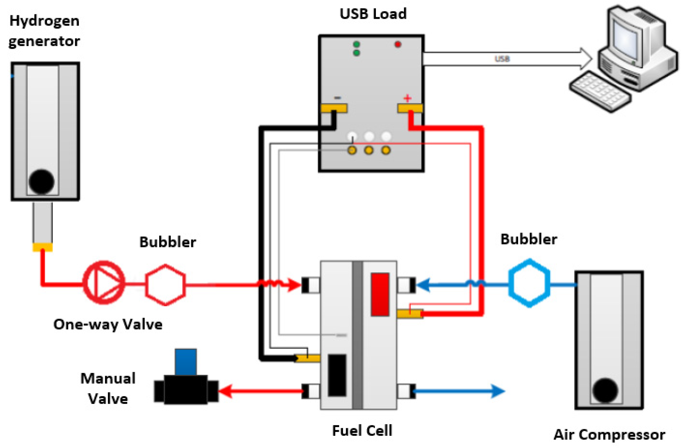
3. Experimental Apparatus

For the experimental validation of the CFD model, an apparatus supplied by the cell manufacturer was adopted. Hydrogen is produced from electrolysis of distilled water using a Hy-PEM XP 2000 (from H2PLANET, 20,069 Italy) electrolyzer, which is connected to the Pragma Industries ClearPak PEMFC via sealed pipes for the hydrogen delivery, presenting non-return valves to ensure a unidirectional flow of the hydrogen produced from the electrolyzer to the cell. The Hy-PEM XP 2000 electrolyzer allows for obtaining a 99.99% pure gas flow with a maximum flow rate of 2000 cc/min, and a pressure regulator for the hydrogen flow allows a pressure up to 16 bar. On the cathode side there is an air compressor for the pressurized cathodic flow, with a control valve to regulate the pressure level. The setup also includes a bubbler, for the inlet gas humidification to guarantee an adequate relative humidity. The test conditions are controlled and data are collected through a LabView data acquisition software system, together with the application of the electrical load to the cell.

The cell is characterized by a Nafion N211 polymeric membrane, which is part of the family of ultra-thin membranes, with a thickness of 25.4 μm. The membrane is assembled with the electrodes in a single piece, the so-called membrane electrode assembly (MEA), characterized by an active surface of 25 cm² and a Pt catalyst load equal to 0.3 mg·cm⁻² at the anode, and 0.6 mg·cm⁻² at the cathode. The testing apparatus provides atmospheric air at cathode and hydrogen at anode (both humidified) and both reactants are at ambient temperature (300 K).

The gas diffusion layers consist of two sheets of carbon fiber with a thickness of 127.3 μm and a porosity equal to 0.5 each, and they are equipped with terminals external to the cell, allowing the application of the externally-imposed electrical potential difference. This device has an applicable potential range between 0 and 5 V, with a resolution of 0.01 V, and a range of circulating current between 0 and 50 A, with a resolution of 0.01 A. In Figure 1 it is possible to see the layout used for the experimental tests. The testing sequence consisted in operating the cell using streams of hydrogen and air, both humidified at saturated conditions by means of the bubblers. The hydrogen flow at anode is at a relative pressure of 0.5 bar and a dead-end blockage is present at anode outlet, consisting of a closed valve to avoid hydrogen leaks from the circuit. The cathode flow of atmospheric air is pressurized at 2 bar and it outflows directly into the atmosphere at cathode outlet section.

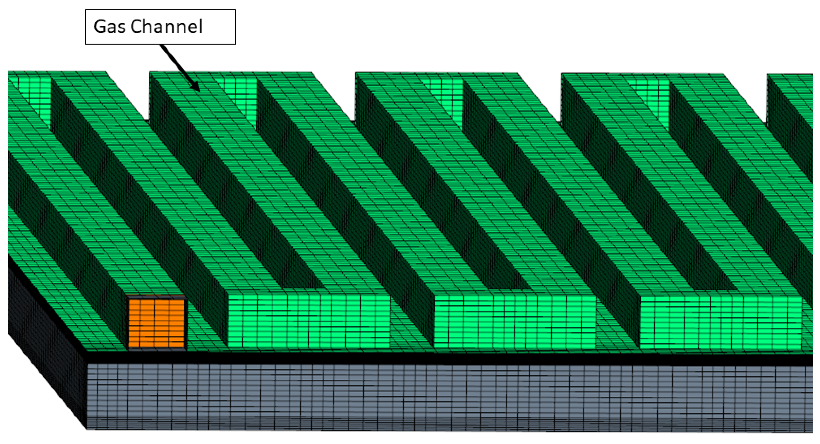
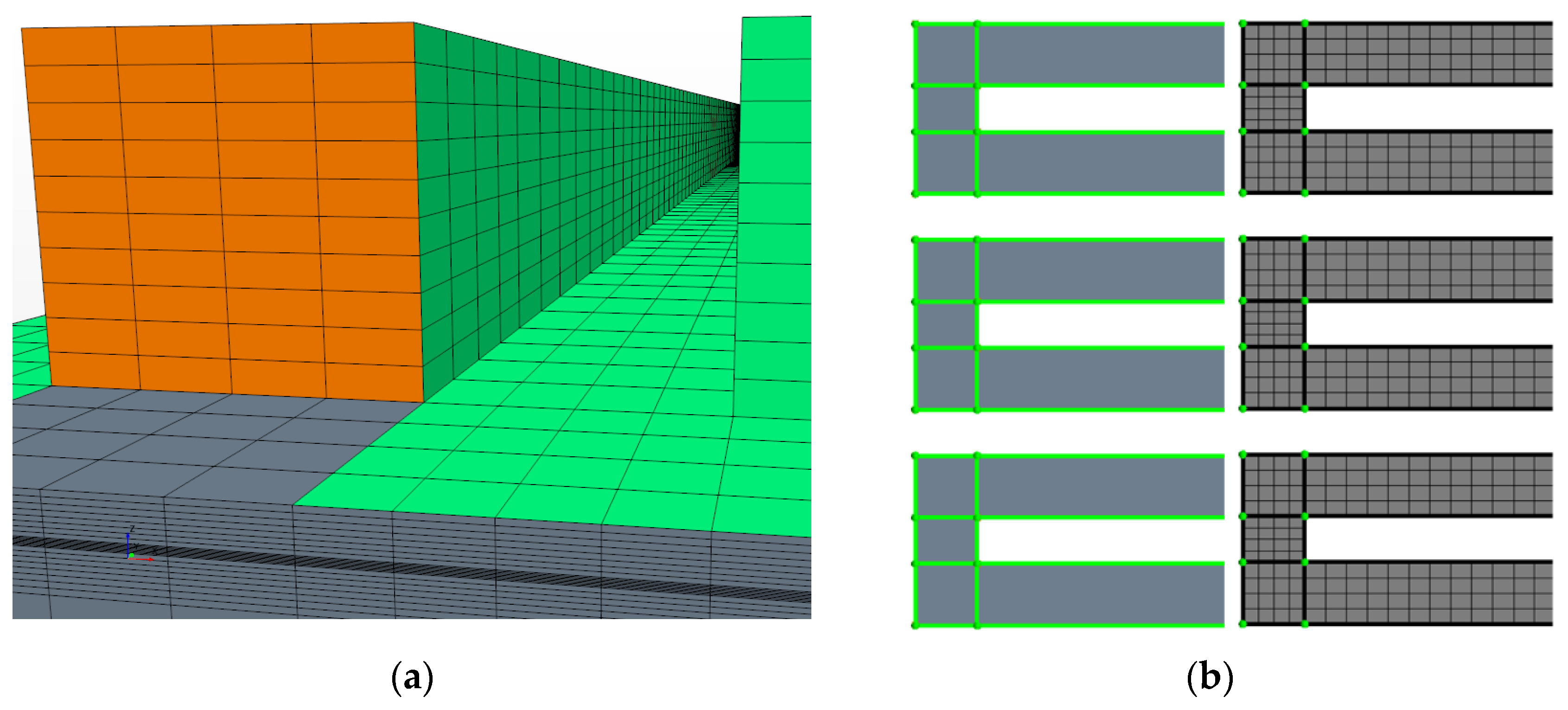
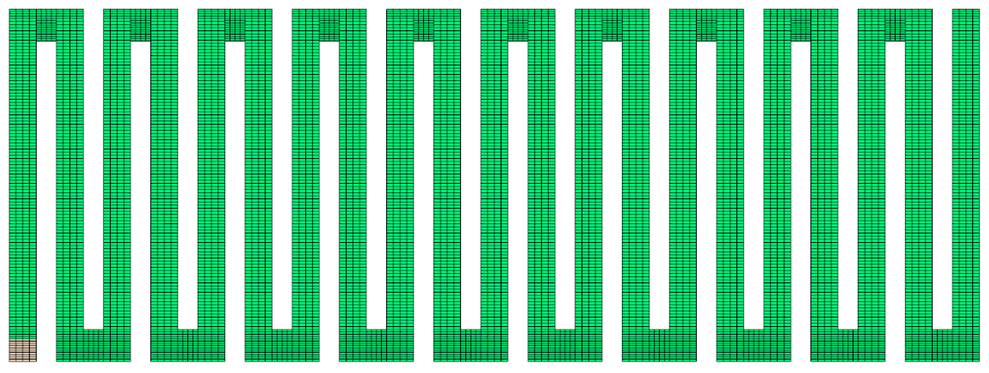
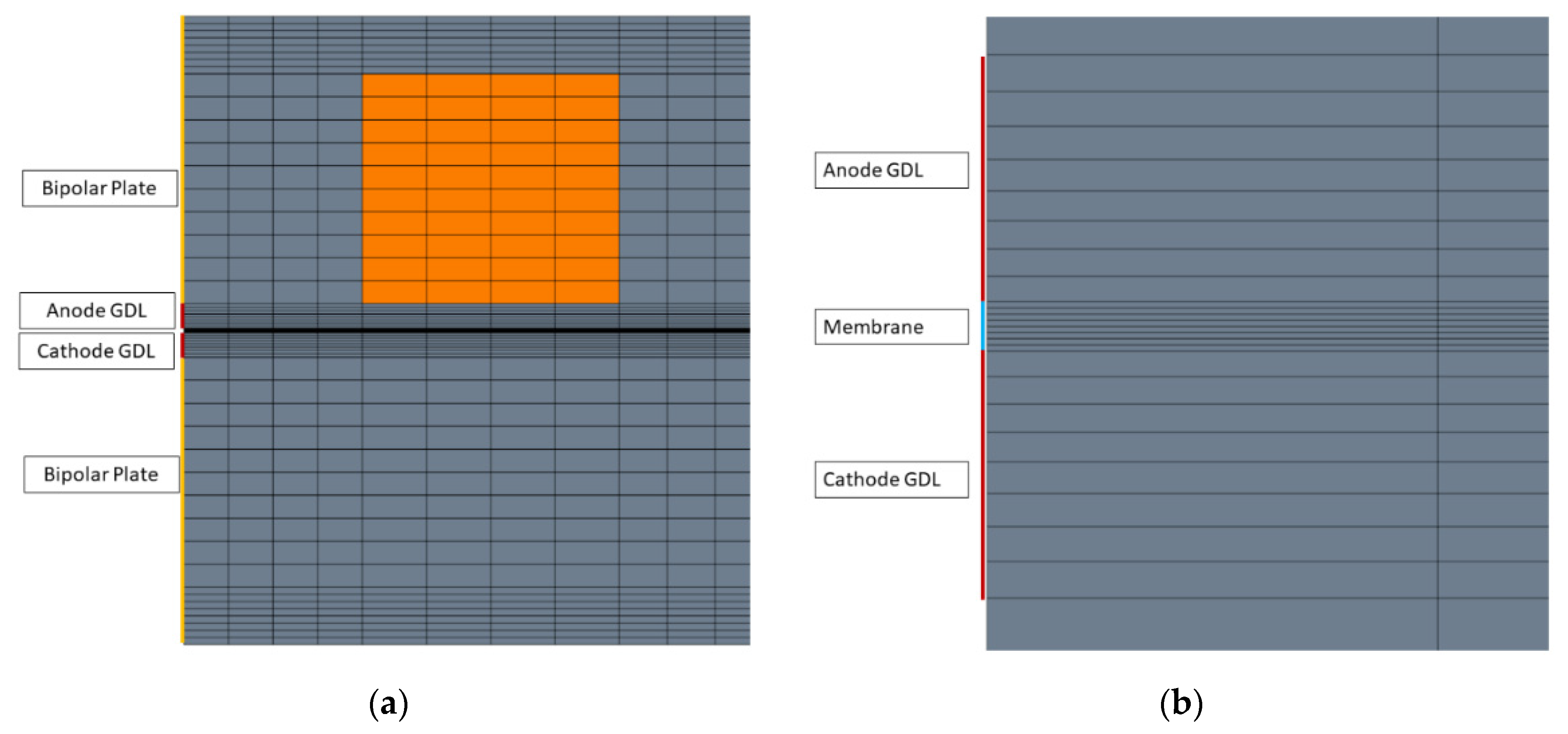
4. D-CFD Model Details

The 3D model for CFD simulations is created using SIMCENTER STAR-CCM+ 2020.2 provided by SIEMENS DISW, and simulations are run with the same package on a 16 CPU Linux workstation. This PEM fuel cell model was also numerically studied in [22]. The characterization of the gas flow at anodic and cathodic channels reproduces the conditions of the laboratory tests, where the cell was supplied with hydrogen and air flows, both humidified with a relative humidity of 100%. The multi-component mixture properties are summarized in

Table 2. Physical properties of cell’s main components.

Domain	Property	Value	Reference
Anode	Relative Humidity (%) Molecular Diffusivity (m2·s−1)	100% $D_{H2}=1.1\times {10}^{-4}; D_{H2O}=7.35\times {10}^{-5}$	[32]
Cathode	Relative Humidity (%) Molecular Diffusivity (m2·s−1)	100% $D_{O2}=3.3\times {10}^{-5} ; D_{N2}=4\times {10}^{-5}$	[32]

, while

Table 3. Parameters of the electrochemical reactions.

Physics	Property	Value	Reference
Anode	Exchange Current Density (A·cm−2) Apparent Charge Transfer Coefficient	$$\begin{gathered} 250\times {10}^{-4} \\ {\alpha }_a=2; {\alpha }_c=2 \end{gathered}$$	[33]
Cathode	Exchange Current Density (A·cm−2) Apparent Charge Transfer Coefficient	$$\begin{gathered} 0.25\times {10}^{-4} \\ {\alpha }_a=2; {\alpha }_c=2 \end{gathered}$$	[33]

reports the constants used to model the electrochemical reactions. The fuel cell polarization curve was measured in the experiments at 100% relative humidity and pressurized flows equal to 0.5 bar at the anode channel and 2 bar at the cathode channel. The operating temperature was 300 K and the circulating current density has been cyclically varied from 0 to 2 A·cm⁻² (via incremental steps of 0.25 A·cm⁻²) to obtain the corresponding voltage and thus defining the characteristic curve of the cell. This is reflected by the boundary conditions used for 3D-CFD simulations, reported in

Table 4. Boundary conditions for the 3D-CFD cell model.

Region	Surface	Property	Value
Anode	Inlet	Mole Fraction Mass Flow (kg·s−1) Pressure (bar) Temperature (K)	$\begin{array}{c}{H}_2:0.9764| H_{2}O :0.0236\\ 3.9175\times {10}^{-7}\\ 1.5\\ 300.15\end{array}$
	Outlet	Mole Fraction Pressure (bar) Temperature (K)	$H_2:0.9764| H_{2}O :0.0236$ 0.5 300.15
Cathode	Inlet	Species Mole Fraction Mass Flow [kg·s−1] Pressure (bar) Temperature (K)	$\begin{array}{c}{O}_2:0.2075\left| N_2=0.7806 \right| H_{2}O :0.0119\\ 2.0728\times {10}^{-5}\end{array}$ 2 300.15
	Outlet	Species Mole Fraction Pressure (bar) Temperature (K)	$O_2:0.2075\left| N_2=0.7806 \right| H_{2}O :0.0119$ 2 300.15

. A three-dimensional model of the tested PEM fuel cell is created for CFD simulations. The discretized grid consists in approximately 1M finite volume cells. In Figure 2 the structured mesh for the anode gas channel mesh and for the cathode bipolar plate are shown. In

Table 5. Parameters of the electrochemical reactions.

Part	Direction	Dimension
Domain	[x;y;z]	[50; 50; 2.68] mm
Gas Channels	Section width	1.34 mm
	Section height	1.2 mm
	Length of serpentine branches	48 mm
	Distance between the serpentine branches	1 mm
GDL	[x;y;z]	[50; 50; 0.1273] mm
Membrane	[x;y;z]	[50; 50; 0.0254] mm

the main dimensions of cell are reported.

The grid creation has been carried out using the Direct Mesh technique both for the channels and for the remaining parts (GDL, membrane, bipolar plates). During the process of defining a structured mesh, a two-dimensional sketch (patch) is created on the origin surface of each component as in Figure 3b. Once the patch has been defined, it is possible to manage the volumetric distribution of the surface mesh along a guide surface (in this case the lateral one), defining the number of cell layers and the parameters of a possible non-homogeneous distribution; this is done through elongation functions, such as the thickness ratio or the ratio between the thicknesses of two adjacent cells. In this way a structured three-dimensional mesh is obtained, such as the one shown as an example in Figure 3a. The Direct Mesh technique allows to have an excellent grid density control and the conformality of the interfaces between the various components, thus ensuring computational efficiency and stability. This grid type is used for all cell components, as visible in Figure 3 and Figure 4. Finally, a high-resolution grid is created in the through-plane direction for GDL (8 layers) and membrane (8 layers), to accurately simulated transport processes in the cell cross-direction. A view of the adopted mesh is reported in Figure 5. Catalyst layers are represented using a thin-layer approach as in [20] and [22], bundling their reaction readiness by exchange current density parameters. This choice is motivated by their ultra-thin cross dimension (10 μm). A higher resolution grid (with twice the resolution in the through-plane direction) was evaluated to assess the effect on the obtained results, and it was discarded given the negligible results variation and the higher computational cost. Steady-state simulations are run until residuals lower than $1 \times {10}^{-7}$ are obtained for all the solved equations.

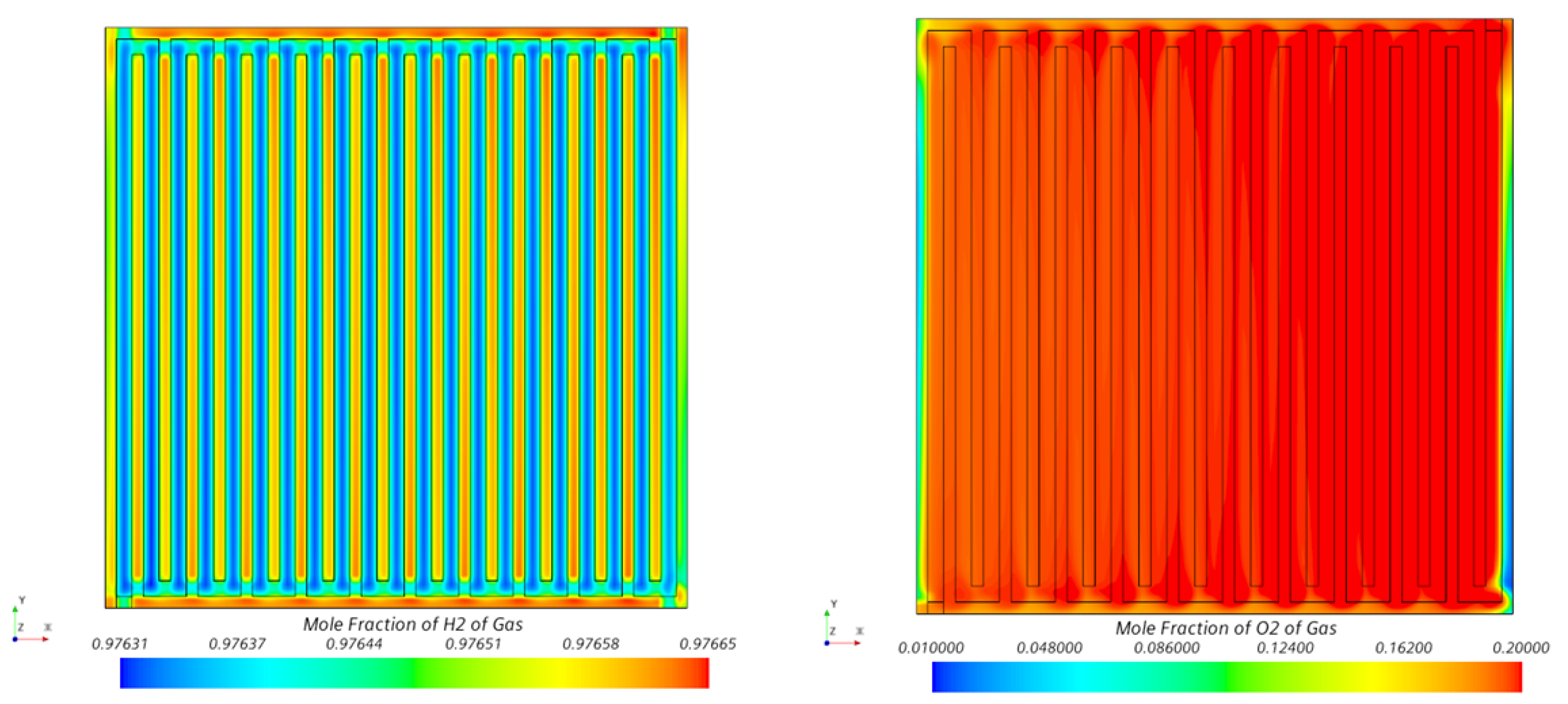
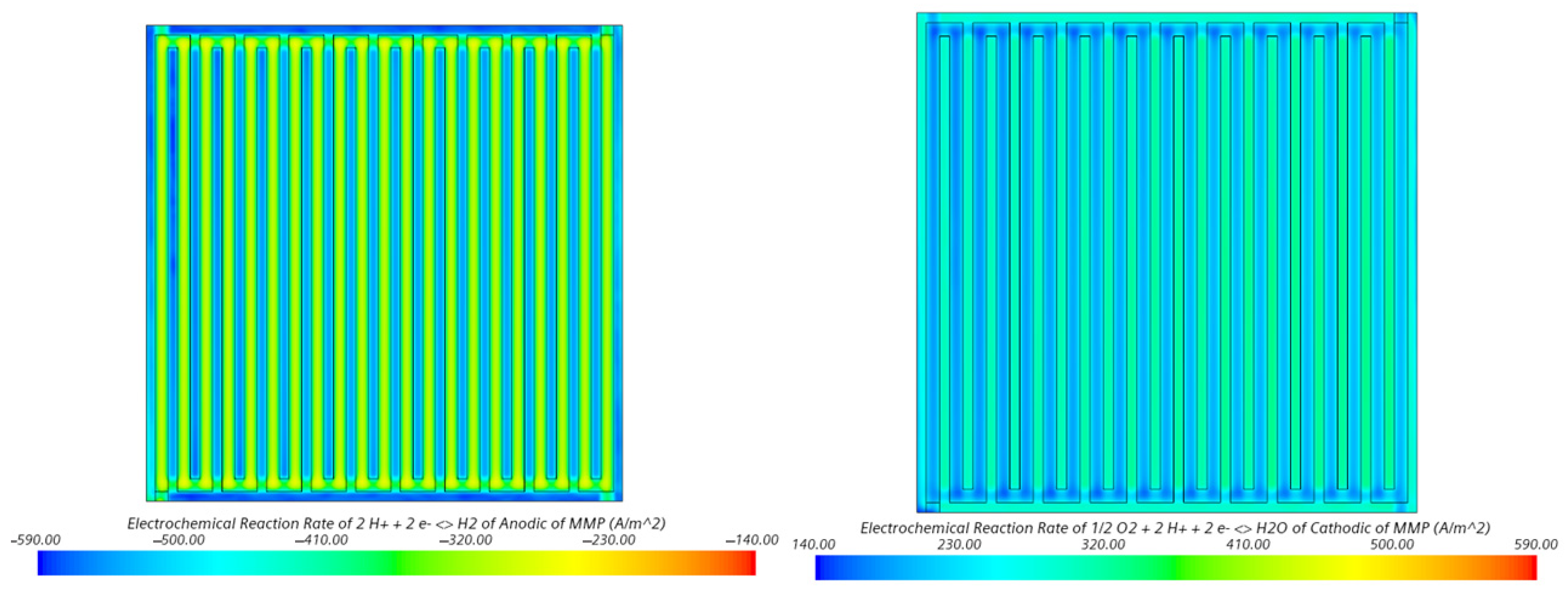
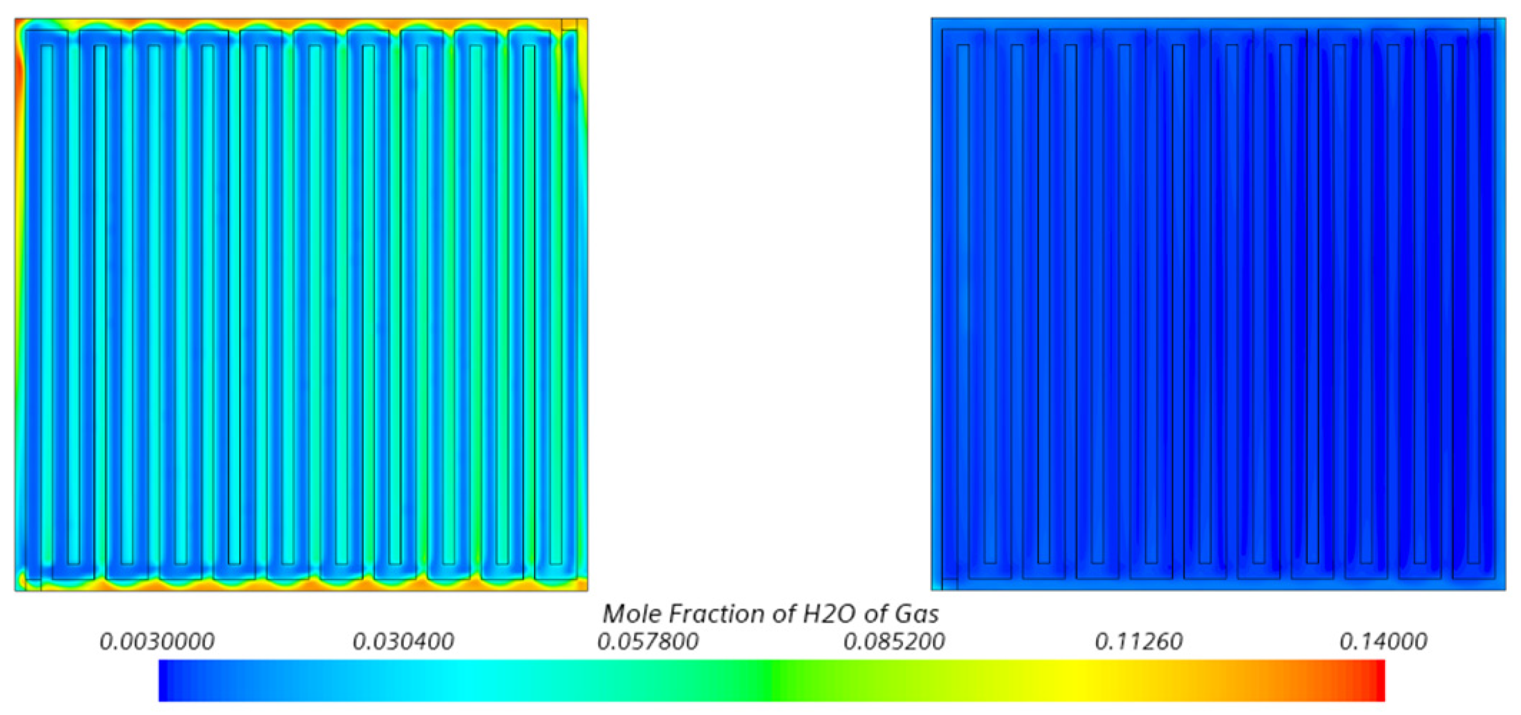
5. Numerical Results

Numerical simulations are carried out for the voltage range from 0.2 to 0.7 V, with 0.1 V steps. In this section the numerical results are reported in detail for the extreme cases, i.e., 0.7 and 0.2 V. Results will focus on species distribution, reaction rate, and thermal gradients, as well as on water formation on the cathode side. Finally, a section will be dedicated to an improved formulation for the exchange current density at cathode, representing a fundamental modelling aspect.

Three-dimensional fields are analyzed for each voltage, which is applied as a boundary condition at the cathode current collector. As shown in Figure 6, hydrogen is consumed from the inlet to the outlet on the side of the anode, while the same is verified for oxygen on the cathode side. The images refer to the 0.7 V configuration and the fields of the molar fractions are extracted at the ACL and to the CCL, respectively, then to the contact interface between the layers of porous diffusion and the polymer membrane. As is visible, the porous GDL allows reactants to distribute over the entire active surface of the catalyst layers for electrochemical reactions, hence its accurate representation is of utmost relevance to reproduce the species diffusivity in this diffusion-dominated region.

The local rate of electrochemical reactions is monitored, and in Figure 7 the electrochemical reaction flux for hydrogen oxidation and oxygen reduction is shown for the 0.7 V case: It is possible to notice areas where the reaction rate is higher, as well as under-used active regions. At the anode side local maxima of reaction rate coincide with minima of $H_2$ concentration (see Figure 6, left), which is consumed by reactions, whereas a more uniform conditions is visible at cathode side both in terms of oxygen concentration (see Figure 6, right) and reaction rate (Figure 7, right). This last aspect is typical of a low current condition, not limited by oxygen availability at CCL. However, in general terms a non-negligible in-plane non-homogeneity of the reaction rate is observed: This is attributed to an insufficient superficial delivery of the reactants (related to the specific reaction rate), essentially motivated by the diffusive-driven transport through the porous layers to the active surface. This may depend on various parameters, including the shape of the channel and its size, as analyzed in [27] on a straight-channel PEM section model.

The 3D-CFD results allow to investigate the formation of liquid water at cathode catalyst layer, as well as modelling the water transport and the hydration state of the membrane, which are essential for high efficiency operation in low-temperature PEMFC. Focusing on water production at the cathode, the two extreme simulated cases are compared in Figure 8, i.e., 0.7 V and 0.2 V cell voltage. In-plane gradients of the water mole fraction at the cathode catalyst layers are visible in both cases and they are related to the inhomogeneity of the cathodic reaction rates (see Figure 7), with the low-voltage/high-current operation leading to higher water production.

The non-isothermal 3D-CFD model also allows to investigate the MEA temperature distribution, illustrated in Figure 9 for the 0.2 V and 0.7 V cases. Both the higher reaction rate (and its associated irreversible heat generation) and the larger current density flowing at CCL in the 0.2 V operation (dissipating more heat via Joule effect) lead to higher temperature for this condition. However, the low-voltage/high-current condition is critical for possible CCL flooding motivated by liquid water production, possibly related due to the super-saturated conditions in the CCL proximity combined with an insufficient water removal rate. Figure 10 highlights how this issue is much less critical at high-voltage/low-current operation, in line with the numerical outcomes in [18,27].

Finally, the measured and simulated polarization curves are reported in Figure 11. As can be seen, a good agreement is found for the current-voltage slope, expressing a satisfactory adherence of the 3D-CFD model to all the potential losses present in the real cell, from activation overpotential (left branch) to Ohmic (central part). As for the concentration losses area (right branch), it is noted that it is almost absent in the measured data. This is explained by the reduced GDL thickness (127.3 μm), leading to a poorly obstructed species transport to/from the catalyst layer active area. The effect of it is the suppression of the concentration losses in the range of the tested conditions. This is reinforced by the same trend observed in both experiments and simulations. A slight underestimation of current density is observed for the numerical model, whose reasons might be a non-perfect material characterization (e.g., the electric conductivity, responsible for linear-type Ohmic overpotential) as well as approximations of electrochemical parameters. Imperfect material characterization is one of the limitations of the present work and further research is in progress, while the accuracy of the cathodic exchange current density is deepened in the next section with an improved formulation for the exchange current density at CCL.

Model Results with Improved Exchange Current Density Formulation

A fundamental parameter in the operating processes of a PEMFC is the exchange current density, characterizing activation losses and for which largely dispersed and non-coherent data are present in literature. In the presented results a constant value was adopted for both the anodic and cathodic reactions ($250\times {10}^{-4}$ and $0.25 \times {10}^{-4}$ A·cm⁻², respectively), which might potentially contribute to the model results deviation in Figure 11. In order to evaluate the effect of an improved correlation on the simulated results, the formulation proposed by Vigna Suria et al. [34] and by Marr et al. [35] are implemented. A constant value is maintained at the anodic side, since the dissociation voltage losses of hydrogen are usually orders of magnitude lower than that of oxygen, whereas a semi-empirical law was adopted for the cathode, able to consider the load of the catalyst layer (i.e., the quantity of platinum particles per surface of the fuel cell, expressed in mg·m⁻²) and the catalyst surface roughness and morphology. In the expressions reported in Equation (27), $K=2.57\times {10}^8$ is a multiplier factor, $m_{pt}$ is the platinum loading on the catalyst layer (g·m⁻²), and $A_s$ is the catalyst surface area, which expresses the area of the active catalytic surface per unit mass of platinum in m²·g⁻¹. Finally, $C_{O2}$ is the mole fraction of oxygen in [mol·m⁻³] divided by a reference concentration $C_{O2,ref}=1.2$ and the local current density $I_{0c}\left(x,y\right)$ is obtained. For the proposed equation, the calculations were carried out using the values reported in

Table 6. Values used for the alternative exchange current density formulation.

Property	Value
Platinum load $m_{pt}$ (g·m−2)	6
Temperature T (K)	300.15
Surface area of the catalyst $A_S$ (m2·g−1)	8

:

$${\log }_{10}\left[I_{0,ref}\left(x,y\right)\right]=3.507-\frac{4001}{T\left(x,y\right)}$$

(26)

$$I_{0c}\left(x,y\right)=K·I_{0,ref}\left(x,y\right)·m_{pt}·A_s·\left(\frac{C_{O2}\left(x,y\right)}{C_{O2,ref}}\right)$$

(27)

The surface area $A_S$ of the catalyst and this parameter depends on many aspects related to humidity, the porosity of the catalyst and the type of used material. From Madhavi et al. [36] it can be deduced that the most suitable value for Nafion in our case is 8 m²·g⁻¹, from which a value for the cathode of $0.337 \times {10}^{-4}$ A·cm⁻² is obtained. The results of the simulations repeated using the exchange current density at cathode are shown in Figure 12. It is possible to observe how in comparison with the starting case, the new value of the exchange current density modifies the resulting polarization and electric power density curves and improves the agreement against the experimental data from the activation-dominated region (i.e., for high-voltage operation) throughout the low-voltage conditions (0.2 V). This motivates the indication of this latter physics-based formulation for the cathodic exchange current density in future 3D-CFD simulations, which is advised to become a standardized practice in multi-dimensional CFD simulation of PEMFC.

6. Conclusions

Fuel cells are considered one of the most promising pathways for a fully sustainable electric mobility and power generation. The attention towards hydrogen-fueled PEMFC is attracting a high interest and relevant research investment, being a key technology to de-carbonize battery-unsuited sectors (e.g., heavy-duty, maritime, aerial, etc.) still relying on the massive use of fossil fuels.

In this paper a hydrogen/air PEM fuel cell is tested and a multi-phase, multi-component, and non-isothermal 3D-CFD model of a PEM fuel cell with a serpentine-type distributor is created, including a diffusive-based model for membrane hydration. Numerical results are compared against experimental data from low to high voltage, recreating the polarization and power density curves. Results are in good agreement with the experiments, although an underestimation of the current density emerges for low-voltage operations, probably due to uncertainty in materials characterization which is part of future research activities. Once a large-scale validation of the results is carried out from characteristic curves (polarization and power density), three-dimensional simulation allows to investigate the interplay of local processes developing inside the cell, such as the spatial distribution of the reactants’ delivery, electrochemical reaction rate, and thermal gradients. High-current/low-voltage operation emerges as the most critical conditions for an adequate supply of reactants at catalyst layers, as well as for the maximized heat generation (both via irreversible and Joule heating mechanisms). In addition, the liquid water generation at the cathode catalyst layer for high-current/low-voltage operation becomes critical at super-saturated low-pressure levels, inducing concentration losses and possibly obstructing the active sites for oxygen reaction. This poses a need to accurately model the porous material characteristics fundamental in the diffusive/capillary-driven removal of liquid water. In the last section, an improved formulation for the exchange current density based on the effective catalyst loading and its active surface area is applied. Results improve with respect to the previous formulation, suggesting this as a recommended guideline for future 3D-CFD models of PEM fuel cells, substituting the still-widespread use of non-Pt-based values for cathodic exchange current density.

The study shows how multi-dimensional CAE models allow a comprehensive understanding of the physical and electrochemical processes in hydrogen-fueled fuel cells, allowing designers to identify limiting processes and virtually exploring innovative high-efficiency configurations.

References

1. Zarei, M.; Davarpanah, A.; Mokhtarian, N.; Farahbod, F. Integrated feasibility experimental investigation of hydrodynamic, geometrical and, operational characterization of methanol conversion to formaldehyde. Energy Sources Part A Recovery Util. Environ. Eff. 2020, 42. [Google Scholar] [CrossRef]
2. Dibazar, S.Y.; Salehi, G.; Davarpanah, A. Comparison of Exergy and Advanced Exergy Analysis in Three Different Organic Rankine Cycles. Processes 2020, 8, 586. [Google Scholar] [CrossRef]
3. Ehyaei, M.A.; Ahmadi, A.; Rosen, M.A.; Davarpanah, A. Thermodynamic Optimization of a Geothermal Power Plant with a Genetic Algorithm in Two Stages. Processes 2020, 8, 1277. [Google Scholar] [CrossRef]
4. Esfandi, S.; Baloochzadeh, S.; Asayesh, M.; Ehyaei, M.A.; Ahmadi, A.; Rabanian, A.A.; Das, B.; Costa, V.A.F.; Davarpanah, A. Energy, Exergy, Economic, and Exergoenvironmental Analyses of a Novel Hybrid System to Produce Electricity, Cooling, and Syngas. Energies 2020, 13, 6453. [Google Scholar] [CrossRef]
5. Valizadeh, K.; Farahbakhsh, S.; Bateni, A.; Zargarian, A.; Davarpanah, A.; Alizadeh, A.; Zarei, M. A parametric study to simulate the non-Newtonian turbulent flow in spiral tubes. Energy Sci. Eng. 2019, 1–16. [Google Scholar] [CrossRef] [Green Version]
6. Davarpanah, A.; Zarei, M.; Valizadeh, K.; Mirshekari, B. CFD design and simulation of ethylene dichloride (EDC) thermal cracking reactor. Energy Sources Part A Recovery Util. Environ. Eff. 2018. [Google Scholar] [CrossRef]
7. Wang, C.-Y. Fundamental Models for Fuel Cell Engineering. Chem. Rev. 2004, 104, 4727–4766. [Google Scholar] [CrossRef]
8. Springer, T.E.; Zawodzinski, S.; Gottesfeld, S. Polymer Electrolyte Fuel Cell Model. J. Electrochem. Soc. 1991, 138, 2334. [Google Scholar] [CrossRef]
9. Bernardi, D.M. A Mathematical Model of the Solid-Polymer-Electrolyte Fuel Cell. J. Electrochem. Soc. 1992, 139, 2477. [Google Scholar] [CrossRef]
10. Kamarajugadda, S.; Mazumder, S. Numerical investigation of the effect of cathode catalyst layer structure and composition on polymer electrolyte membrane fuel cell performance. J. Power Sources 2008, 183, 629–642. [Google Scholar] [CrossRef]
11. Feser, J.P.; Prasad, A.K.; Advani, S.G. On the relative influence of convection in serpentine flow fields of PEM fuel cells. J. Power Sources 2006, 161, 404–412. [Google Scholar] [CrossRef]
12. Pharoah, J.G. On the permeability of gas diffusion media used in PEM fuel cells. J. Power Sources 2005, 144, 77–82. [Google Scholar] [CrossRef]
13. Zeng, Z.; Grigg, R. A Criterion for Non-Darcy Flow in Porous Media. Transport. Porous Media 2006, 63, 57–69. [Google Scholar] [CrossRef]
14. Zhang, X.; Chen, S.; Xia, Z.; Zhang, X.; Liu, H. Performance Enhancements of PEM Fuel Cells with Narrower Outlet Channels in Interdigitated Flow Field. In Proceedings of the ICAE2018—The 10th International Conference on Applied Energy, Hong Kong, China, 22–25 August 2018. [Google Scholar] [CrossRef]
15. Um, S.; Wang, C.Y. Three-dimensional analysis of transport and electrochemical reactions in polymer electrolyte fuel cells. J. Power Sources 2004, 125, 40–51. [Google Scholar] [CrossRef]
16. Yang, Y.-L. Performance of a low-cost direct glucose fuel cell with an anion-exchange membrane. Int. J. Hydrog. Energy. 2015, 40, 10979–10984. [Google Scholar] [CrossRef]
17. Carcadea, E.; Varlam, M.; Ismail, M.; Ingham, D.B.; Marinoiu, A.; Raceanu, M.; Jianu, C.; Patularu, L.; Ion-Ebrasu, D. PEM fuel cell performance improvement through numerical optimization of the parameters of the porous layers. Int. J. Hydrog. Energy 2020, 45, 7968–7980. [Google Scholar] [CrossRef]
18. Tabuchi, Y.; Shiomi, T.; Aoki, O.; Kubo, N.; Shinohara, K. Effects of heat and water transport on the performance of polymer electrolyte membrane fuel cell under high current density operation. Electrochim. Acta 2010, 56, 352–360. [Google Scholar] [CrossRef]
19. Hashemi, F.; Rowshanzamir, S.; Rezakazemi, M. CFD simulation of PEM fuel cell performance: Effect of straight and serpentine flow fields. Math. Comput. Model. 2012, 55, 1540–1557. [Google Scholar] [CrossRef]
20. Berning, T.; Lu, D.M.; Djilali, N. Three-dimensional computational analysis of transport phenomena in a PEM fuel cell. J. Power Sources 2002, 106, 284–294. [Google Scholar] [CrossRef]
21. Zhang, G.; Xie, X.; Xuan, J.; Jiao, K.; Wang, Y. Three-Dimensional Multi-Scale Simulation for Large-Scale Proton Exchange Membrane Fuel Cell; SAE Technical Paper 2019-01-0381; SAE International: Warrendale, PA, USA, 2019. [Google Scholar] [CrossRef]
22. Ferreira, R.B.; Falcão, D.S.; Oliveira, V.B.; Pinto, A. 1D + 3D two-phase flow numerical model of a proton exchange membrane fuel cell. Appl. Energy 2017, 203, 474–495. [Google Scholar] [CrossRef]
23. Kulikowsky, A.A. Analytical Modelling of Fuel Cells; Elsevier: Amsterdam, The Netherlands, 2010. [Google Scholar]
24. Jiao, K.; Li, X. Water transport in polymer electrolyte membrane fuel cells. Prog. Energy Combust. Sci. 2011, 37, 221–291. [Google Scholar] [CrossRef]
25. Wu, H.; Li, X.; Berg, P. On the Modeling of Water Transport in Polymer Electrolyte Membrane Fuel Cells. Electrochem. Acta 2009, 54, 6913–6927. [Google Scholar] [CrossRef]
26. Djilali, N. Computational modelling of polymer electrolyte membrane (PEM) fuel cells: Challenges and opportunities. Energy 2007, 32, 269–280. [Google Scholar] [CrossRef]
27. D’Adamo, A.; Riccardi, M.; Locci, C.; Romagnoli, M.; Fontanesi, S. Numerical Simulation of a High. Current Density PEM Fuel Cell; SAE Technical Paper 2020-24-0016; SAE International: Warrendale, PA, USA, 2020. [Google Scholar] [CrossRef]
28. Riccardi, M.; D’Adamo, A.; Vaini, A.; Romagnoli, M.; Borghi, M.; Fontanesi, S. Experimental Validation of a 3D-CFD Model of a PEM Fuel Cell. E3S Web Conf. 2020, 197. [Google Scholar] [CrossRef]
29. Leverett, M.C. Capillary behavior in porous solids. Trans. AIME 1941, 142, 151–169. [Google Scholar] [CrossRef]
30. Kumbur, E.C.; Sharp, K.V.; Mench, M.M. Validated Leverett Approach for Multiphase Flow in PEFC Diffusion Media: I. Hydrophobicity Effect. J. Electrochem. Soc. 2007, 154, 1295. [Google Scholar] [CrossRef]
31. Ye, Q.; Nguyen, T.V. Three-Dimensional Simulation of Liquid Water Distribution in a PEMFC with Experimentally Measured Capillary Functions. J. Electrochem. Soc. 2007, 154, 1242. [Google Scholar] [CrossRef]
32. Macedo-Valencia, J.; Sierra, J.M.; Figueroa-Ramìrez, S.J.; Dìaz, S.E.; Meza, M. 3D CFD modeling of a PEM fuel cell stack. Int. J. Hydrog. Energy 2016, 41, 23425–23433. [Google Scholar] [CrossRef]
33. Sivertsen, B.R.; Djilali, N. CFD-based modelling of proton exchange membrane fuel cells. J. Power Sources 2005, 141, 65–78. [Google Scholar] [CrossRef]
34. Vigna Suria, O.; Testa, E.; Peraudo, P.; Maggiore, P. A PEM Fuel Cell Distributed Parameters Model. Aiming at Studying the Production of Liquid Water Within the Cell During its Normal Operation: Model. Description, Implementation and Validation; SAE Technical Paper 2011-01-1176; SAE International: Warrendale, PA, USA, 2011. [Google Scholar] [CrossRef]
35. Marr, C.; Li, X. Composition and Performance Modelling of Catalyst Layer in a Proton Exchange Membrane Fuel Cell. J. Power Sources 1999, 77, 17–27. [Google Scholar] [CrossRef]
36. Madhavi, B.; Sanket, G.; Balaji, K. Platinum utilization in proton exchange membrane fuel cell and direct methanol fuel cell. J. Electrochem. Sci. Eng. 2019, 9, 281–310. [Google Scholar] [CrossRef]
Figure 1. Layout and components of the experimental tests.
Processes 09 00564 g001
Figure 2. Mesh distribution in the anode gas channel (green, with anode bipolar plate removed for visualization) and in the cathode bipolar plate (grey).
Processes 09 00564 g002
Figure 3. (a) Computational Direct mesh of the serpentine. (b) Patch mesh of the serpentine.
Processes 09 00564 g003
Figure 4. Mesh of the serpentine on the anode side.
Processes 09 00564 g004
Figure 5. (a) Mesh distribution on the interface between bipolar plates and GDLs and (b) between GDLs and membrane.
Processes 09 00564 g005
Figure 6. Section views of hydrogen (left, anode side) and oxygen (right, cathode side) mole fraction fields for the 0.7 V case at CL surfaces.
Processes 09 00564 g006
Figure 7. Section views of electrochemical reaction flux at anode (left) and cathode (right) for the 0.7 V case.
Processes 09 00564 g007
Figure 8. Section views of H 2 O mole fraction at CCL for the 0.2 V (left) and the 0.7 V case (right).
Processes 09 00564 g008
Figure 9. Section views of temperature at CCL for the 0.2 V (left) and the 0.7 V case (right).
Processes 09 00564 g009
Figure 10. Section views of liquid volume fraction at CCL for the 0.2 V (left) and the 0.7 V case (right).
Processes 09 00564 g010
Figure 11. Polarization curve and electric power density for experiments and simulations.
Processes 09 00564 g011
Figure 12. Polarization curve and electric power density for experiments and simulations, including the results using the improved exchange current density formulation (Equation (27)).
Processes 09 00564 g012