Optimization Design of a Two-Vane Pump for Wastewater Treatment Using Machine-Learning-Based Surrogate Modeling

Abstract

This paper deals with three-objective optimization, using machine-learning-based surrogate modeling to improve the hydraulic performances of a two-vane pump for wastewater treatment. For analyzing the internal flow field in the pump, steady Reynolds-averaged Navier-Stokes equations were solved with the shear stress transport turbulence model as a turbulence closure model. The radial basis neural network model, which is an artificial neural network, was used as the surrogate model and trained to improve prediction accuracy. Three design variables related to the geometry of blade and volute were selected to optimize concurrently the objective functions with the total head and efficiency of the pump and size of the waste solids. The optimization results obtained by using the model showed highly accurate prediction values, and compared with the reference design, the optimum design provided improved hydraulic performances.

1. Introduction

Recently, with the increase in the usage of disposable masks because of the COVID (Corona virus disease)-19 pandemic, used masks are being commonly discarded in toilets. If the cloth wastes such as a disposable mask or large waste such as a baby diaper is disposed into a toilet, the flow path of the pump that transports wastewater is blocked, and as a result, the function of the wastewater transport system is lost. Therefore, the demand for special pumps for wastewater transportation is increasing, and it has gained attention as an industry with the potential for future growth.

As an example of the special pumps, grinder and vortex pumps are widely used for transporting wastewater. However, these special pumps have low efficiency and high maintenance costs, contributing to large operating costs. Several studies explored the treatment of sewage containing solid waste to solve these problems [1,2,3,4]. Lu et al. [1] studied the hydraulic performance and pressure fluctuation characteristics of a grinder pump. Through a numerical analysis, the hydraulic performances of the pump when the flow path is in a clogging state and in a normal operating state were compared, and steady and unsteady Reynolds-averaged Navier-Stokes (RANS) analyses was performed. It was found that, as the degree of clogging of the grinder cutter increases, the total head of the pump declines parabolically, with the best efficiency point shifting to the low flow rate region and the high efficiency area narrowing. Schivley and Dussourd analyzed and designed a vortex pump, using a one-dimensional analytical model [2]. They compared the calculated performance parameters with those measured by using the laboratory model, and they computed the overall hydraulic characteristics of the pump and compared these characteristics with those of many test pumps. They improved the theoretical formula used in the preliminary design of a vortex pump. Ohba et al. [3] theoretically analyzed the flow characteristics inside a vortex pump and secured the theoretical reliability by comparing the predicted values with experimental results. Their theoretical formula could predict not only the hydraulic performance of the vortex pump, but also the velocity component inside the pump. The obtained results were in good agreement with the experimentally measured values. Steinmann et al. [4] analyzed the internal flow of a vortex pump through numerical analysis and experiments to investigate the unsteady cavitating flow of a vortex pump. The Rayleigh–Plesset cavitation model was used to simulate cavitation under the overload condition of the vortex pump, and an acrylic glass window was installed in the experimental apparatus, to observe this phenomenon. Under the best efficiency point condition, the numerically derived head and shaft power of the pump were about 6% higher than the experimentally measured values. Conversely, cavitation under overload was observed more in experimental results than in numerical analysis.

In addition to the grinder and vortex pumps mentioned above, single-channel pumps designed to transport relatively larger solid wastes were actively studied [5,6,7]. The single-channel impeller with a single free annulus passage can smoothly transfer sewage-containing solid wastes. However, this impeller has an unsymmetrical annulus flow passage, and it is difficult to stabilize the unsteady flow-induced vibration, due to the interaction between the rotating impeller and stationary volute [5]. Shi and Tsukamoto [6] numerically analyzed the pressure fluctuation due to the impeller–diffuser interaction in a diffuser pump. They confirmed that the flow characteristics due to this interaction can be analyzed through an unsteady flow analysis. Feng et al. [7] analyzed the unsteady flow characteristics between the impeller and diffuser of a radial pump by unsteady RANS (URANS) analysis and laser Doppler velocimetry (LDV); they identified two types of rotor–stator interaction effects. One is the downstream effect induced by the impeller, which has an unsteady flow characteristic because of the highly distorted flow field and the wake of the impeller. The other is the upstream effect induced by the stator, which causes unsteady pressure and velocity fluctuations. Such a single-channel pump has the advantage of being able to transport relatively large waste solids, but it has the disadvantage that the fluid-induced vibration is greater than that in the existing special pumps (e.g., grinder and vortex pumps) because of its asymmetric structural characteristics.

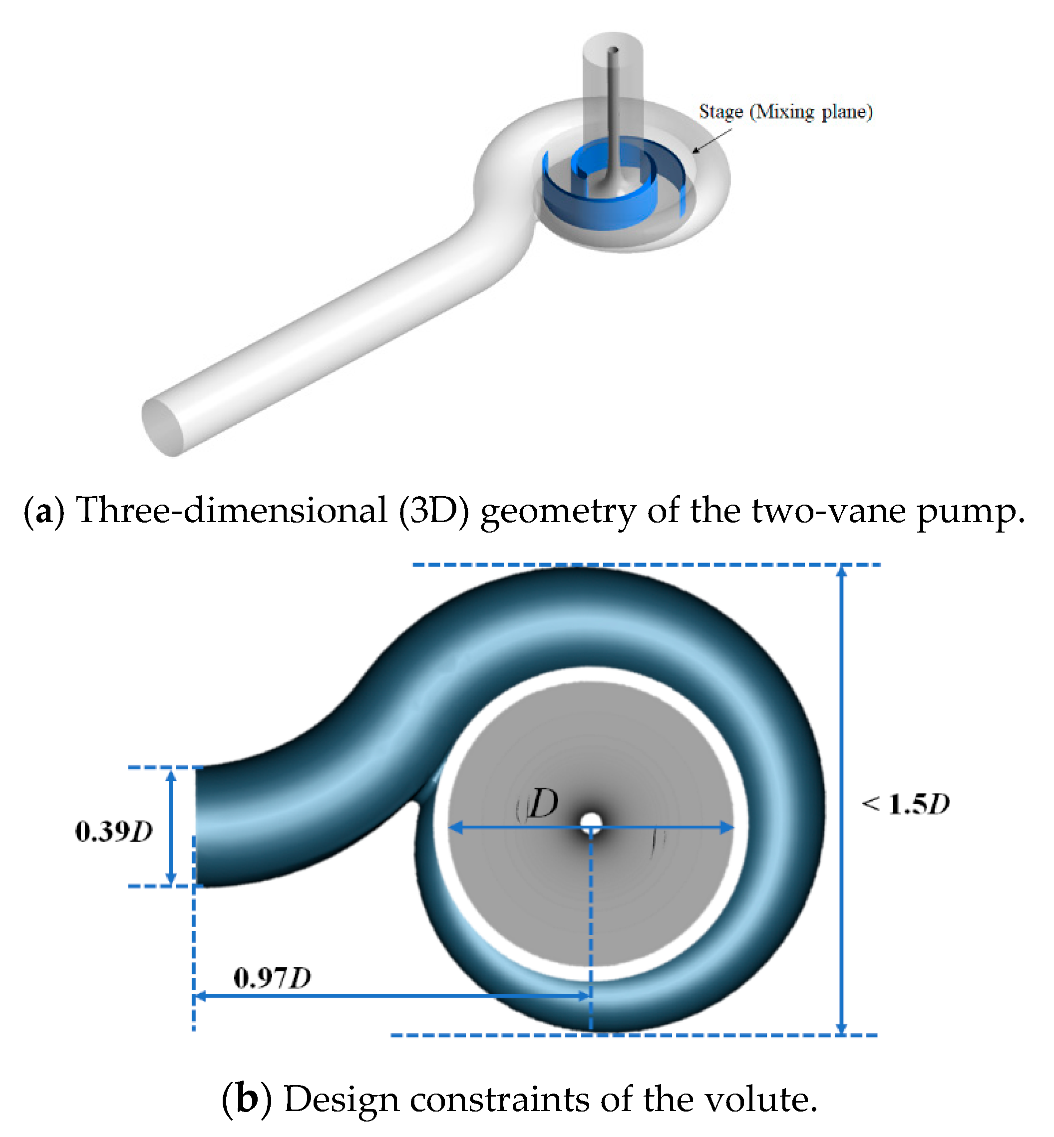
The special pumps for wastewater treatment introduced so far clearly have advantages and disadvantages, depending on their type. Grinder and vortex pumps have low vibration during operation, but the size of transportable solid matters is relatively small, and the maintenance costs are relatively high. On the other hand, a single-channel pump can easily transport large solid matters, but in some cases, relatively severe vibration occurs. To solve these problems, the authors intended to design a two-vane pump in this study. The impeller of the two-vane pump is composed of two blades that are symmetrical in the rotational axis. Therefore, it is structurally simple compared to the grinder and vortex pumps, and the relatively large flow path of the impeller has a small number of blades, so waste solids can be transferred smoothly. In addition, due to the symmetrical impeller geometry, the fluid-induced vibration is relatively less than that of a single-channel pump.

In the past, design optimization using numerical analysis has been widely used for fluid-based machinery [8,9,10,11]. For example, Lee et al. [10] performed an optimization to improve the efficiency of a low-speed axial flow fan, using a gradient-based search algorithm. Lee and Kim [11] optimized axial compressor blades to improve the efficiency, using numerical optimization techniques such as conjugate direction methods and the golden section method, combined with a three-dimensional (3D) thin-layer Navier-Stokes solver. Recently, with the rapid advances in computing resources, optimal design is being actively researched based on machine-learning techniques [12,13].

In this study, a two-vane pump was designed to develop a series of special pumps for transporting wastewater. Compared to a single-channel pump, this pump can transport relatively smaller waste solids but experiences less vibration during operation because of the axial symmetry of the impeller. Considering the characteristics of this pump, a three-objective optimization design based on machine learning was performed to maximize the size of the waste solids that can be transported while simultaneously improving the hydraulic performances of the pump. For the three-objective optimization, the geometric design variables, i.e., inlet and outlet blade angles and cross-sectional area of the volute, were chosen, and the volume of the waste solids and the head and efficiency of the pump were considered as objective functions. Their relationship was predicted by using an artificial neural network (ANN) [14] based on machine learning. Then, the genetic algorithm (GA) [15] was used to find the optimal solutions, and the Pareto-optimal front surface [16] was derived as the final optimization result.

2. Numerical Methods

2.1. Two-Vane Pump Model

The preliminary two-vane pump model used in this work was designed by using CFturbo [17], under the following design conditions: a flow rate of 0.5 m³/min, a total head of 10 m, and a rotational speed of 1760 rpm (revolution per minute).

The two-vane pump used in this study was designed for commercialization, and the preliminary design was carried out to satisfy the “KS B 6301 Standard” that requires the performance certification on fresh water under 35 °C, as the national certification system for the centrifugal pumps, including sewage types in the Republic of Korea. Therefore, the preliminary design and optimization of the pump were conducted to satisfy the design specifications when the working fluid is fresh water.

In this study, the initial impeller of the two-vane pump had two blades, as shown in Figure 1, and a diameter of 207 mm. The blades are shrouded impeller blades, and there is no tip clearance. The inlet and outlet blade angles are 6.50° and 8.00°, respectively, and have identical values from the hub to the shroud. To prevent the special case that the textile or cloth material caught on the blade, the ellipse ratio of the leading and trailing edge of the blade is designed to 1.0. Figure 1b shows the volute geometry and design constraints. Since the pump used in this study was installed through a manhole of the city water and sewage system, there are some constraints on the overall size of the pump and outlet diameter, as shown in Figure 1b.

The preliminary model has a specific speed (N_s) of 221.3 in SI (International system of units) units (rpm, m³/min, m) under the design conditions. The specific speed formula used in this study is as follows:

$$N_s=\frac{N\times \sqrt{Q}}{{\left[H_t\right]}^{3/4}}$$

(1)

where N, Q, and H_t denote the rotational speed, flow rate, and total head of the pump, respectively. Figure 2 is a diagram for helping designer to roughly judge the theoretical efficiency according to the specific speed of the pump in SI unit. Now, the type of the pump can be determined by the specific speed, as shown in Figure 2, and the efficiency can be estimated by using the following approximation formula [18]:

$$\mathsf{\eta }=\left[0.94-0.294264\times {\left[\frac{Q}{N}\times X\right]}^{-0.21333}-12.893\times {\left[{\log }_{10}\left(\frac{2286}{N_s}\right)\right]}^2\right]\times 100 (\%)$$

(2)

$$\mathrm{X}={\left[\frac{3.56}{\epsilon }\right]}^2$$

(3)

where ε is the absolute roughness height of the pump surfaces. It depends on the production processes and materials. In this study, the milling and die-casting methods that are commonly used in pump processing were assumed, and, accordingly, ε was calculated as 7.84 μm [18]. That is, according to Equations (2) and (3), the efficiency under design condition of the preliminary model is predicted to be about 71%.

However, based on the numerical analysis of the preliminary model, the total head was predicted as about 18 m at the design flow rate, and the specific speed was calculated as 142; these values do not satisfy the design specifications. In addition, for a specific speed of 142, the efficiency will be about 65%, as shown in Figure 2. To solve this problem, by applying the similarity law, the impeller diameter was reduced by about 13%, compared to the preliminary model, and optimization was performed to improve the hydraulic performances.

2.2. Numerical Analysis

The 3D RANS equations were solved by using a k-ω-based shear stress transport (SST) turbulence model [19] for the hydraulic analysis of the two-vane pump. The SST turbulence model is known to be suitable for predicting flow separation due to an adverse pressure gradient near the wall, and the k-ω turbulence model [20] and the k-ε turbulence model [21] are applied near the wall and to the bulk flow region, respectively. These two turbulence models are connected by the blending function that is influenced by the y⁺ value—the dimensionless number representing the distance between the wall and the first node of the grid system [19].

Commercial code ANSYS CFX 19.1 [22] was used for the RANS analysis. The computational domain is shown in Figure 1a. The 3D geometry of the impeller was created by using ANSYS Blade-Gen [22], and the volute was created by using Solidworks 2016 [23]. ANSYS TurboGrid and ICEM [22] were used to generate the computational grids for the rotating and stationary domains, respectively. The stage (or mixing plane) method was applied at the interface between the rotating and stationary domains to calculate a steady-state solution for the problems of multiple reference frames [22].

The working fluid was water at 25 °C. The total pressure was set to 1 atm as the atmosphere condition at the inlet boundary. The numerical analysis was performed by assigning the mass flow rate to the outlet boundary. The blade and volute surfaces in the computational domain were considered to be hydraulically smooth under an adiabatic and no-slip condition.

The grid system used in the present study consists of hexahedral grids in the rotating domain and tetrahedral grids in the stationary domain, as shown in Figure 3. In the rotating domain, O-type grids were constructed around the blades. To determine the convergence of the numerical calculations, the root-mean-square values of the residuals of the governing equations were set to be less than 10⁻⁵. The physical time scale was set to 1/ω, where ω is the angular velocity of the impeller. The computation for the steady RANS analysis was performed, using an Intel Xeon CPU with a clock speed of 2.70 GHz, and converged solutions were obtained after 1000 iterations with a computational time of approximately 8 h.

3. Optimization Techniques

The three-objective optimization problem was defined as follows:

• Maximize: F(x) = [F₁(x), F₂(x), F₃(x)]
• Design variable bound: LB ≤ x ≤ UB, x∈R,

where F(x) is the vector of real-valued objective functions; x is the vector of the design variables; LB and UB denote the vectors of the lower and upper bounds, respectively; and R is a real number [24].

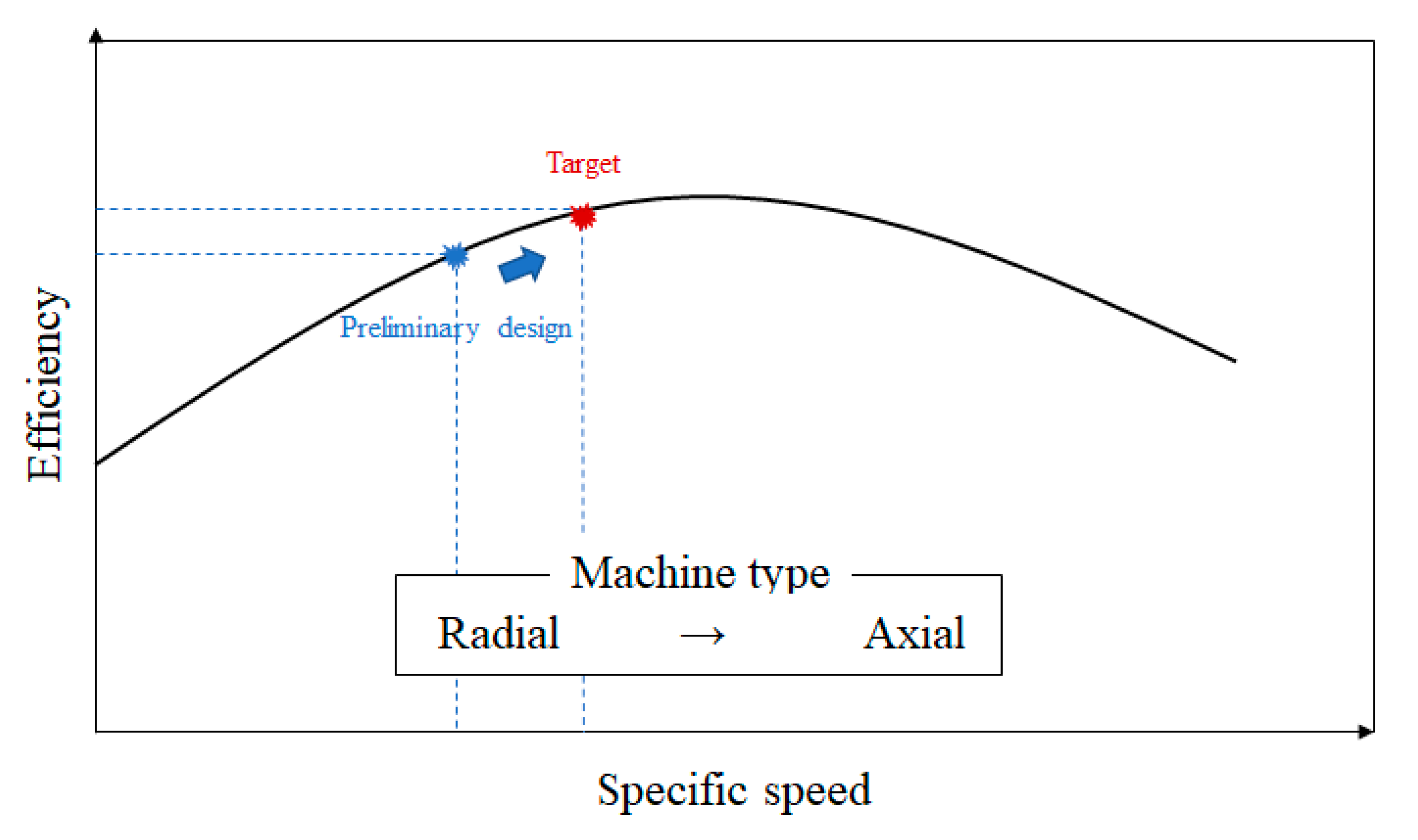
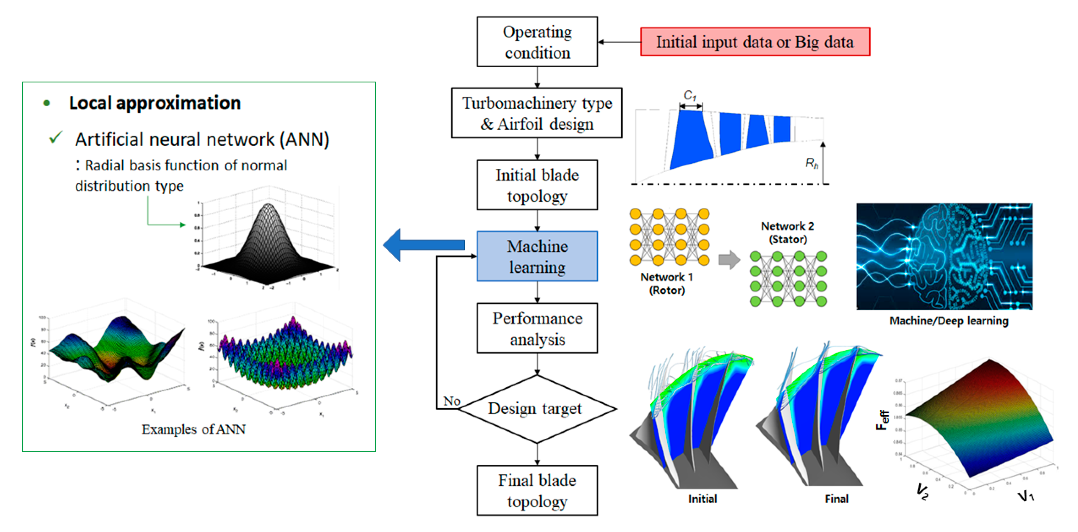
Figure 4 shows the procedure of a typical optimization design. Once the operating conditions of the design target are determined, the type of turbomachinery and airfoil (or hydrofoil) are selected. Then a preliminary design is performed through one-dimensional mean-line analysis, and the initial blade topology is derived. Subsequently, the optimization design is performed for improving the performance of the turbomachinery.

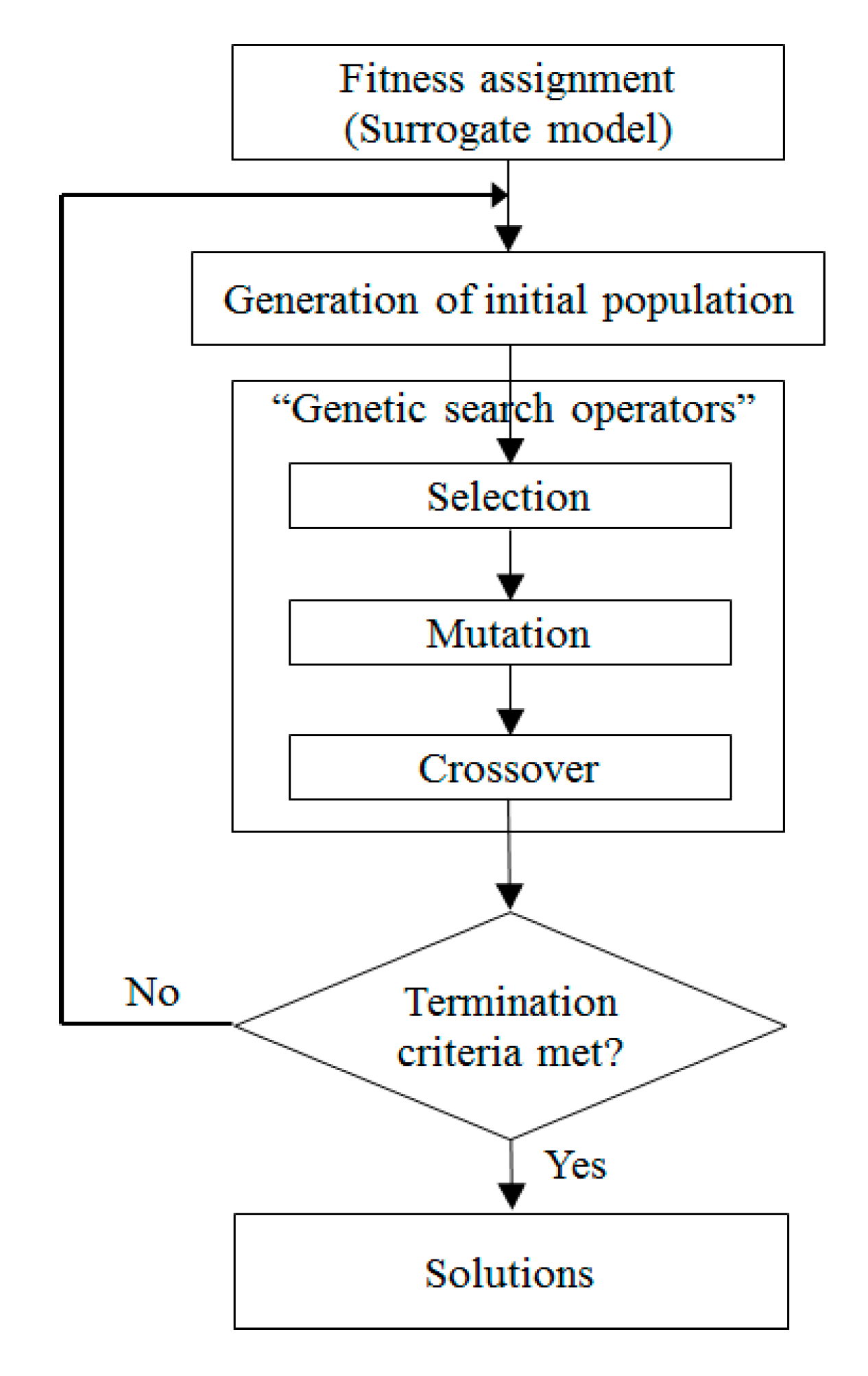
In this study, the optimization design was based on machine learning. First, the objective functions and constraints were defined according to the design goal. Subsequently, the design variables and their ranges were chosen. Thereafter, a database of the correlation between the design variables and the objective functions was established within the design space, using the design of experiment (DOE). In the next step, a predictive model was constructed by using ANN [14] to correlate the design variables and objective functions of the two-vane pump. In this step, the predictive model was trained by using machine learning. This process is described in detail in Section 3.2. The GA [15] was used to find the optimal design solution, considering the correlation of each objective function in the constructed prediction model. The GA is a well-known stochastic searching algorithm based on the mechanism of natural selection, genetics, and evolution. It evaluates various points in the design space and can be applied to find a global solution to any given problem. This algorithm proceeds as shown in Figure 5. Finally, the Pareto-optimal front surface was derived by using MATLAB R2018b [25], and the optimization procedure was terminated.

3.1. Design Variables and Objective Functions

In order to maximize the hydraulic performances and size of waste solids, the efficiency (η) and total head (H_t) of the pump and the volume of waste solids (V_s) were selected as the objective functions:

$$H_t=\frac{P_{outlet}-P_{ inlet}}{\rho g}$$

(4)

$$\eta =\frac{\left(P_{outlet}-P_{ inlet}\right)Q}{\tau \omega }\times 100\%$$

(5)

$$V_s=\frac{1}{6}\pi D_s^3$$

(6)

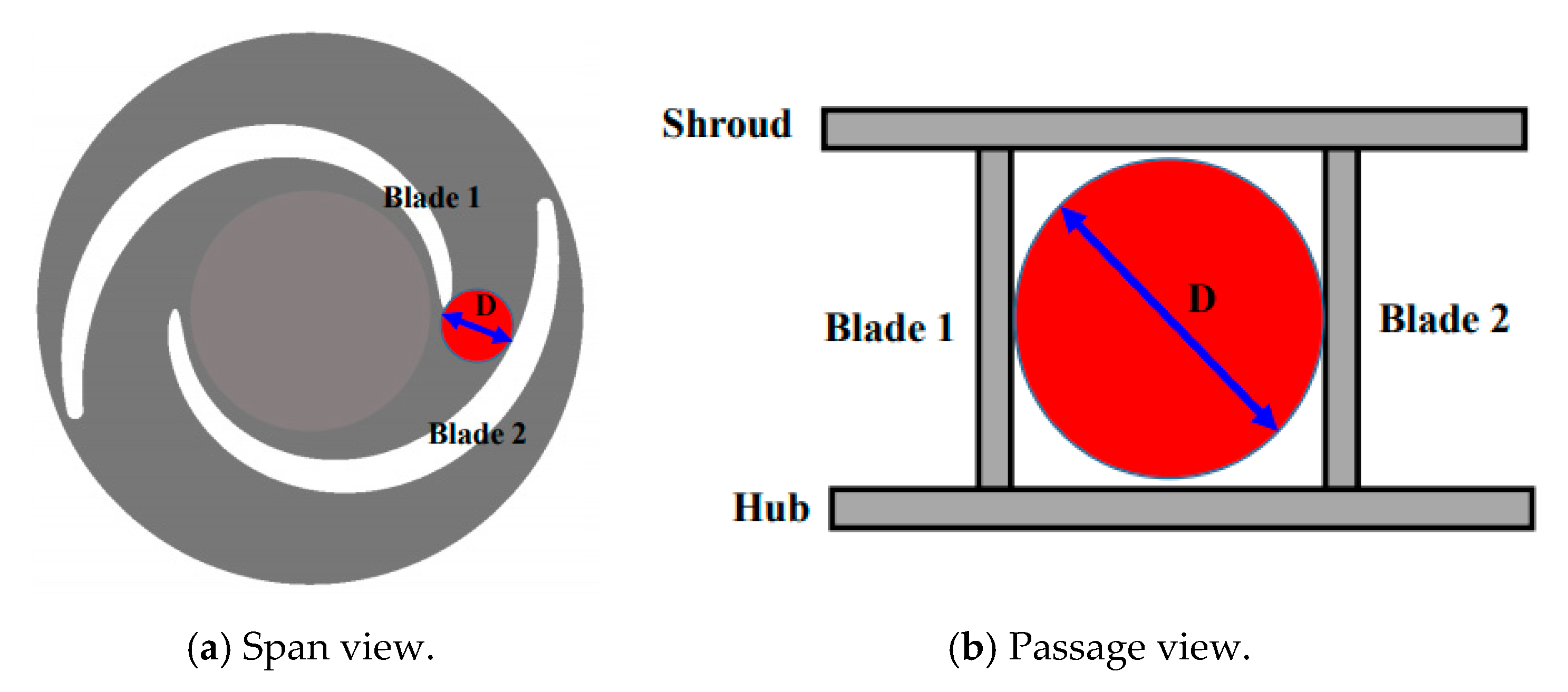
where P, ρ, g, Q, τ, and ω are the total pressure, density of the working fluid, acceleration due to gravity, flow rate, torque, and angular velocity, respectively. Further, D_s in Equation (6) is defined as the distance between the leading edge of the blade and the other blade at the impeller inlet, as shown in Figure 6.

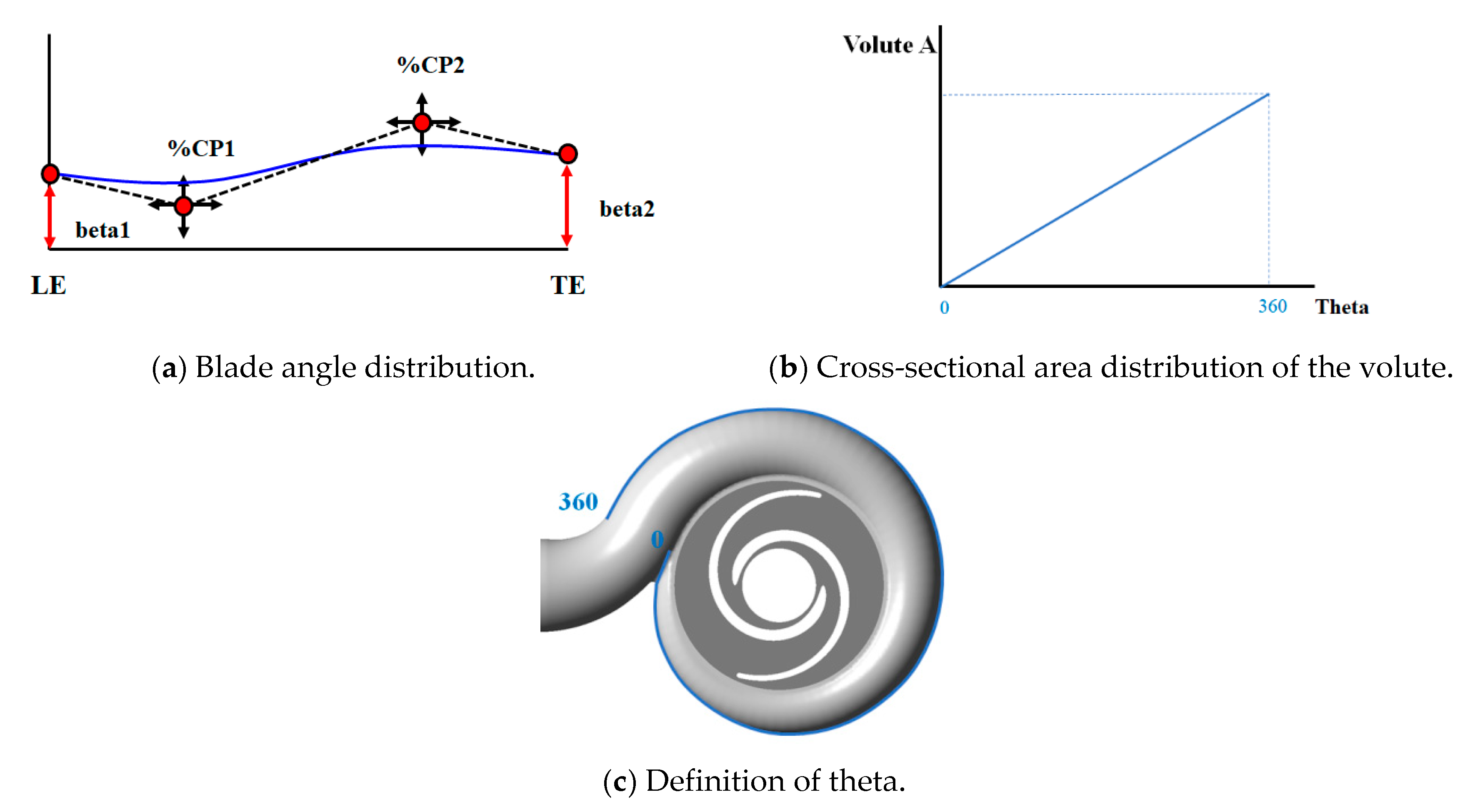
Figure 7 shows the design variables considered in this work. Their ranges are listed in

Table 1. Ranges of design variables.

	LB	Ref.	UB
β1/β1,ref	0.483	1.00	1.517
β2/β2,ref	0.119	1.00	1.381
Volute A/Aref	0.813	1.00	1.187

LB = lower bound; UB, upper bound.

. The inlet and outlet blade angles and the cross-sectional area of the volute were chosen for the optimization. They are defined as shown in Figure 7. As mentioned earlier, the blade angle distribution is the same in the span direction from the hub to the shroud and is defined by using the fourth-order Bézier curve [26] in the streamwise direction, as shown in Figure 7a. In order to adjust the inlet (β₁) and outlet (β₂) blade angles, two control points (CP₁ and CP₂) were fixed. The distribution of the cross-sectional area of the volute was changed linearly in the circumferential direction, as shown in Figure 7b.

3.2. Surrogate Modeling Based on Machine Learning

In the present optimization design, supervised machine learning was adopted, considering the reasonable computation costs. This optimization technique is a very efficient approach for optimizing a system without analytical representation, fitting a surrogate model.

In order to construct the input data, the central composite design was used as the DOE. In all, 15 experimental points were arranged for three design variables, and the objective function values were derived through RANS analysis at each design point. These values are listed in

Table 2. Initial input data for the supervised machine learning.

	β1/β1,ref	β2/β2,ref	Volute A/Aref	Ht/Ht,ref	η/ηref	Vs/Vs,ref
1	0.692	0.375	0.889	0.669	1.075	0.111
2	1.308	0.375	0.889	0.666	1.059	1.125
3	0.692	1.125	0.889	0.684	1.037	0.111
4	1.308	1.125	0.889	0.683	1.030	1.260
5	0.692	0.375	1.111	0.643	1.008	0.111
6	1.308	0.375	1.111	0.650	1.009	1.125
7	0.692	1.125	1.111	0.663	0.959	0.111
8	1.308	1.125	1.111	0.659	0.979	1.260
9	0.483	0.750	1.000	0.669	0.914	1.004
10	1.517	0.750	1.000	0.649	0.941	1.728
11	1.000	0.119	1.000	0.645	1.089	0.512
12	1.000	1.381	1.000	0.693	0.997	0.593
13	1.000	0.750	0.813	0.690	1.103	0.512
14	1.000	0.750	1.187	0.646	1.017	0.512
15	1.000	0.750	1.000	0.666	1.008	0.512

. In this table, the values of the design variables and objective functions are normalized by dividing them by the corresponding reference value.

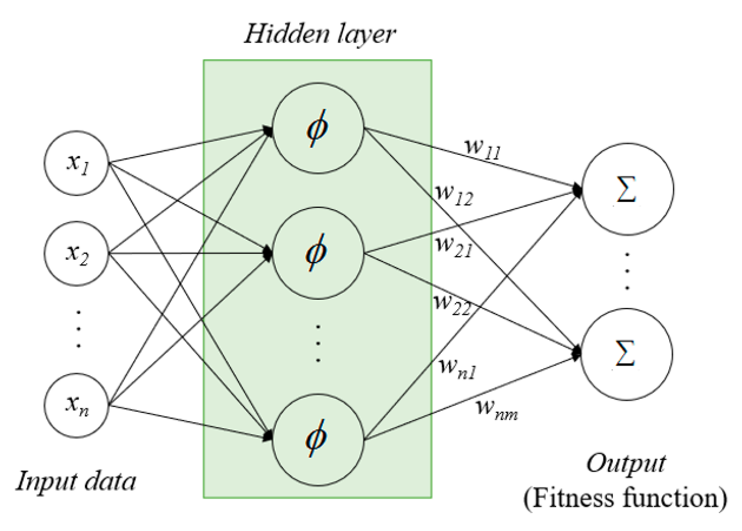
A radial basis neural network (RBNN) model [27], which is a type of ANN, was used in this optimization study. The RBNN model has a hidden layer of radial neurons and an output layer of linear neurons, as shown in Figure 8. The hidden layer uses a series of radial primitives to nonlinearly modify the input space to the intermediate space. The output of the hidden layers then executes a linear combiner to produce the desired targets [27]:

$$f\left(\mathrm{x}\right)={\displaystyle \sum }_{j=1}^N{w}_j{\varphi }_j$$

(7)

where w_j is the weight, and φ_j is radial basis function, which uses the Gaussian function. Several parameters are needed to construct a surrogate model: the input weight and the center and width of a unit for the Gaussian function. In the present RBNN model, the input weights were chosen by machine learning. 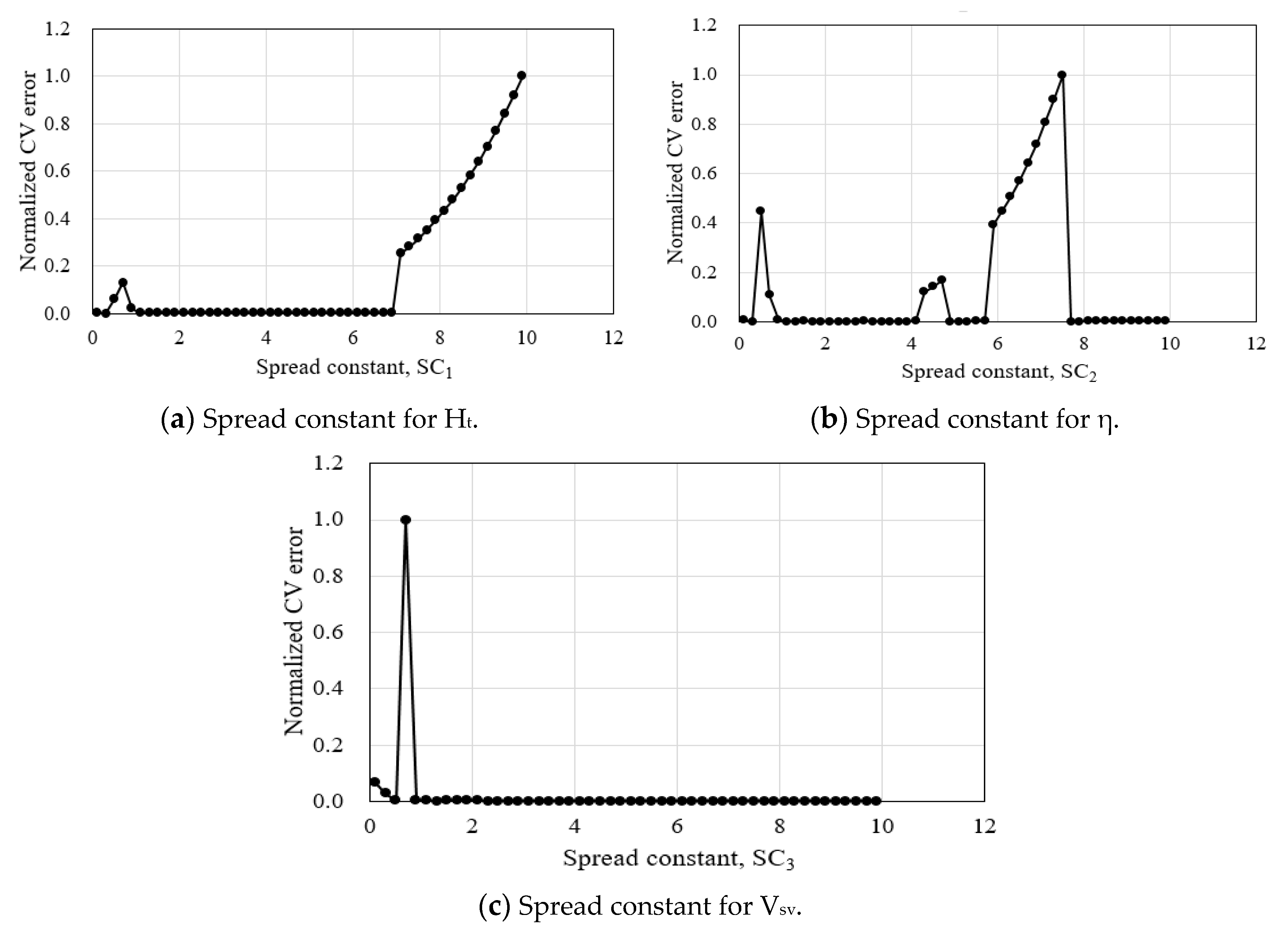The input vector with the worst performance was chosen as the center of a new hidden-layer Gaussian function [25]. Then the RBNN only needed to determine the width of the Gaussian function (spread constant). The network training was performed by adjusting the cross-validation error (CV) by changing the spread constant (SC), as shown in Figure 9. SC₁, SC₂, and SC₃ correspond to the total head, efficiency, and size of waste solids, respectively. The SC values for each objective function were chosen by a K-fold CV test [28].

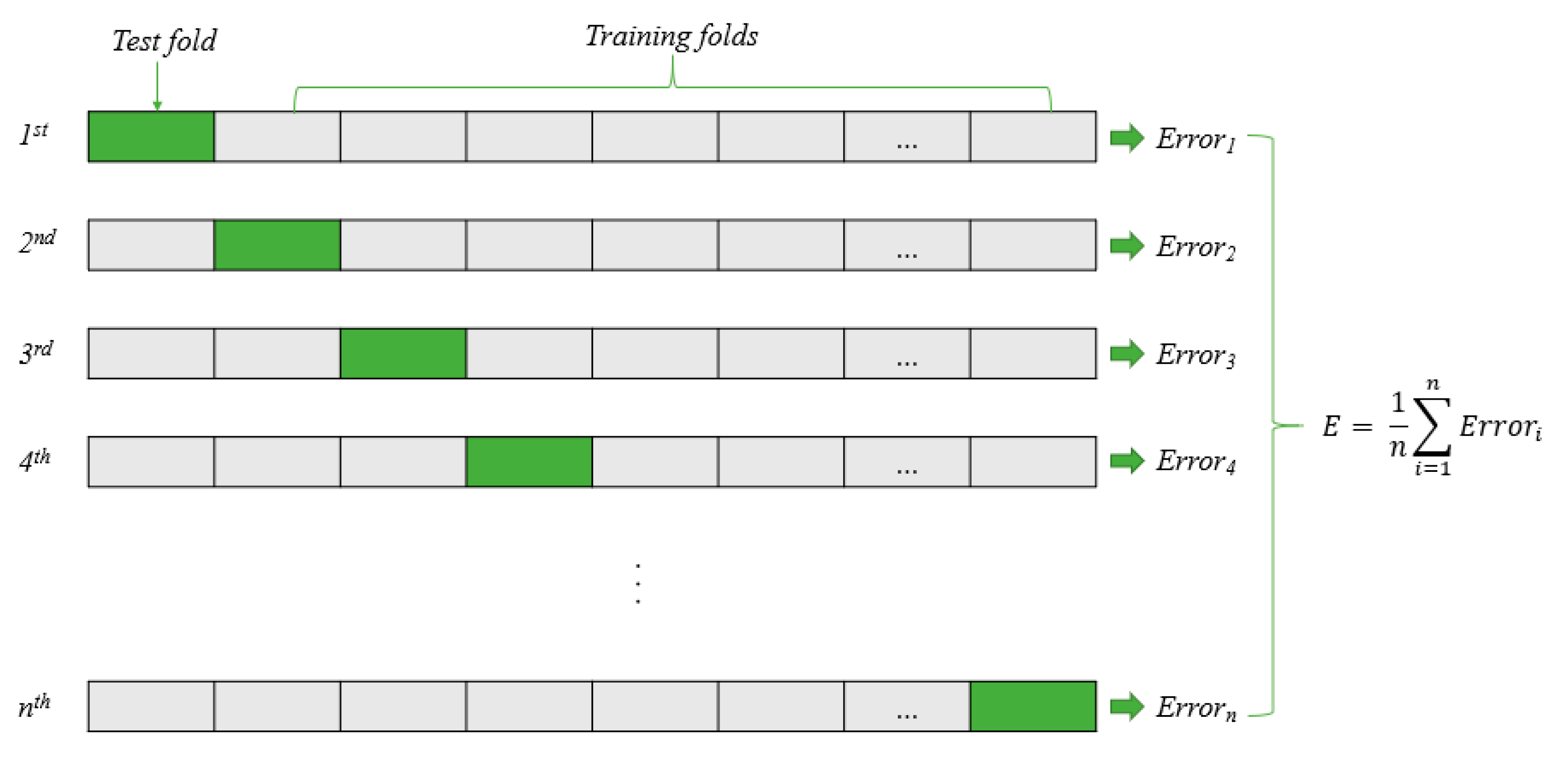
The data sample $((x_j,y_j); j=1,\dots ,\mathrm{N})$ was partitioned into K disjoint subsets (K-fold CV), as shown in Figure 10. Of these, (K-1) folds were used to train the RBNN network, and the last fold (the Kth set) was used for evaluation. This process was repeated K times, using a different fold for evaluation each time. The network training was performed by adjusting the CV error by changing SC. The CV error at a particular SC value was calculated as follows:

$$\mathrm{CV}\left(\mathrm{SC}\right)=\frac{1}{\mathrm{K}}{\sum }_{i=1}^k{\in }_k, {\in }_k={\sum }_{j=kth set}{(y_j-{\widehat{y}}_j)}^2,$$

(8)

where ${\in }_k$ is the prediction error for the Kth set. The predicted values ${\widehat{y}}_j$ were determined by using the constructed RBNN model from the sample points in the (K-1) subsets. In the present study, K was set as 15. According to the results of the K-fold CV test, the final SC values SC₁, SC₂, and SC₃ were set as 0.3, 1.9, and 9.9, respectively.

4. Results

4.1. Grid Dependency Test and Validation of Numerical Results

To eliminate the grid dependency of the numerical solutions, grid dependency tests were performed in the computational domain, as shown in Figure 11. In these tests, the efficiency and total head under the design condition were compared, and their values were normalized by dividing by the corresponding convergence values. As shown in Figure 11, the grid system with 3.4 × 10⁶ nodes undergoes only 0.002% and 0.083% changes in the efficiency and total head, respectively, compared with the grid system with 3.0 × 10⁶ nodes. Hence, the latter grid system was selected as the optimal grid system for the computational domain.

In earlier research, the authors analyzed the internal flow characteristics of hydraulic machines, such as pumps and water turbines, through numerical analysis and compared and verified the numerical results through experiments [29,30,31,32]. In a previous study, a single-channel pump with design specifications similar to those of the two-vane pump considered in this study was developed, and Figure 12 shows the results of the experiments conducted in the previous study [29]. The hydraulic performances, i.e., the head coefficient and efficiency, were compared with the corresponding experimental data in the operating ranges. The total head values derived from the numerical analysis were almost identical to the experimental data. Meanwhile, the efficiency values were relatively higher than those of the experimental data because the numerical analysis did not include the mechanical losses. However, the general trend of the efficiency curve matched well. In this study, the numerical scheme used in the previous studies of the authors [29,30,31,32] was adopted, and the numerical analysis technique was verified through several peer reviews. The results derived of this study will be verified through experiments in future work.

4.2. Optimization Results

Figure 13 shows the Pareto-optimal front surface for the three-objective optimization. This surface was obtained by using the GA based on the RBNN predictive model. To investigate the accuracy of the optimization results, five arbitrary optimal designs (AODs) were selected. They are listed in

Table 3. Optimization results.

	Design Variables			Predicted Values			RANS
	β1/β1,ref	β2/β2,ref	Volute A/Aref	Ht/Ht,ref	η/ηref	Vs/Vs,ref	Ht/Ht,ref	η/ηref	Vs/Vs,ref
AOD 1	1.514	1.357	0.818	0.647	1.082	2.171	0.676	1.048	2.097
AOD 2	1.432	0.122	0.814	0.643	1.126	1.603	0.654	1.135	1.260
AOD 3	1.289	0.128	0.815	0.648	1.148	1.185	0.654	1.151	1.000
AOD 4	1.046	0.137	0.820	0.651	1.163	0.636	0.650	1.164	0.593
AOD 5	0.943	0.165	0.820	0.654	1.159	0.457	0.652	1.147	0.439

RANS = Reynolds-averaged Navier-Stokes.

and shown in Figure 13.

The objective functions of the predicted AODs were calculated by RANS analysis and compared with the predicted objective function values listed in Table 3. The RANS results indicate that the maximum relative errors were less than 1.90% for the total head, 1.80% for the efficiency, and 4.00% for the size of waste solids. Thus, the surrogate model is regarded as being constructed based on reliable data, and the results of optimization indicate the excellent accuracy of surrogate prediction.

All the AODs are predicted to have a normalized total head of more than 0.611, which satisfies the design target, and the efficiency and the size of waste solids are inversely related. In addition, all the AODs have less cross-sectional area of the volute, compared to the reference design, and the efficiencies of the AODs are improved. The design focused on the size of waste solids (AOD 1) doubles the solid size compared with that in the reference design, whereas the design focused on efficiency (AOD 5) shows an increment of 14.14% in the efficiency.

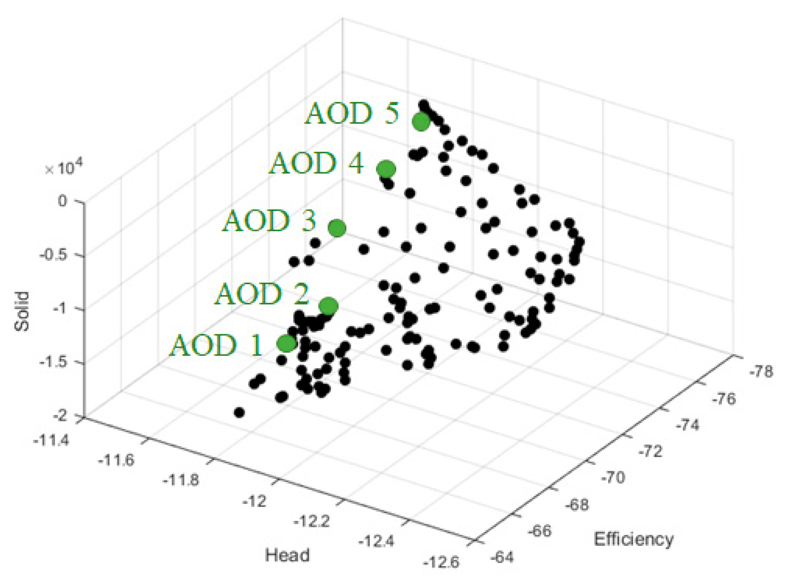
5. Discussion

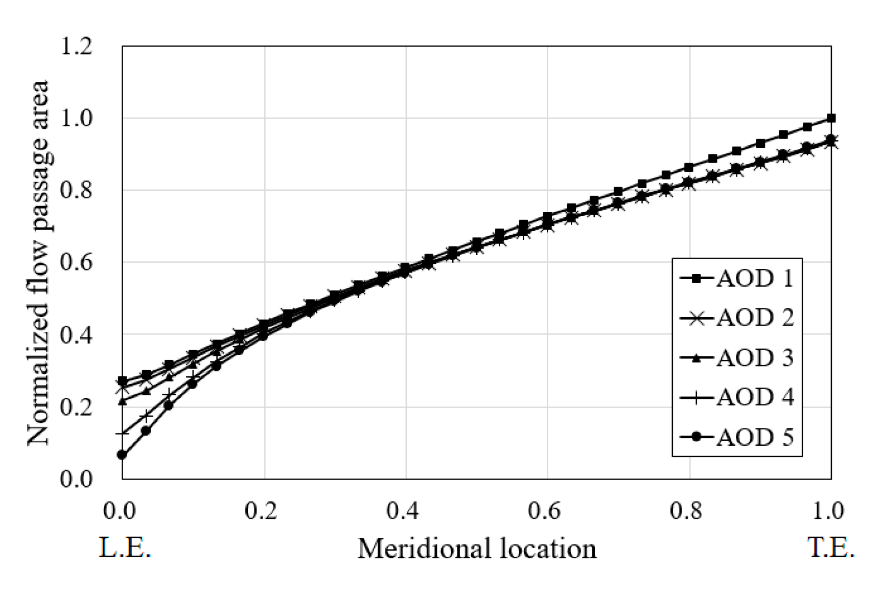
The size of waste solids is directly related to the blade inlet angle. As the blade inlet angle increases, the size of waste solids increases. The flow passage areas of the AODs in the meridional direction are compared in Figure 14. Their values are normalized by using the maximum area of AOD 1 in the meridional direction. It was confirmed that the inlet passage area of AOD 1 with the greatest increase in the blade inlet angle was the largest, and the inlet passage area of AOD 5 with the reduced inlet blade angle was the smallest among AODs.

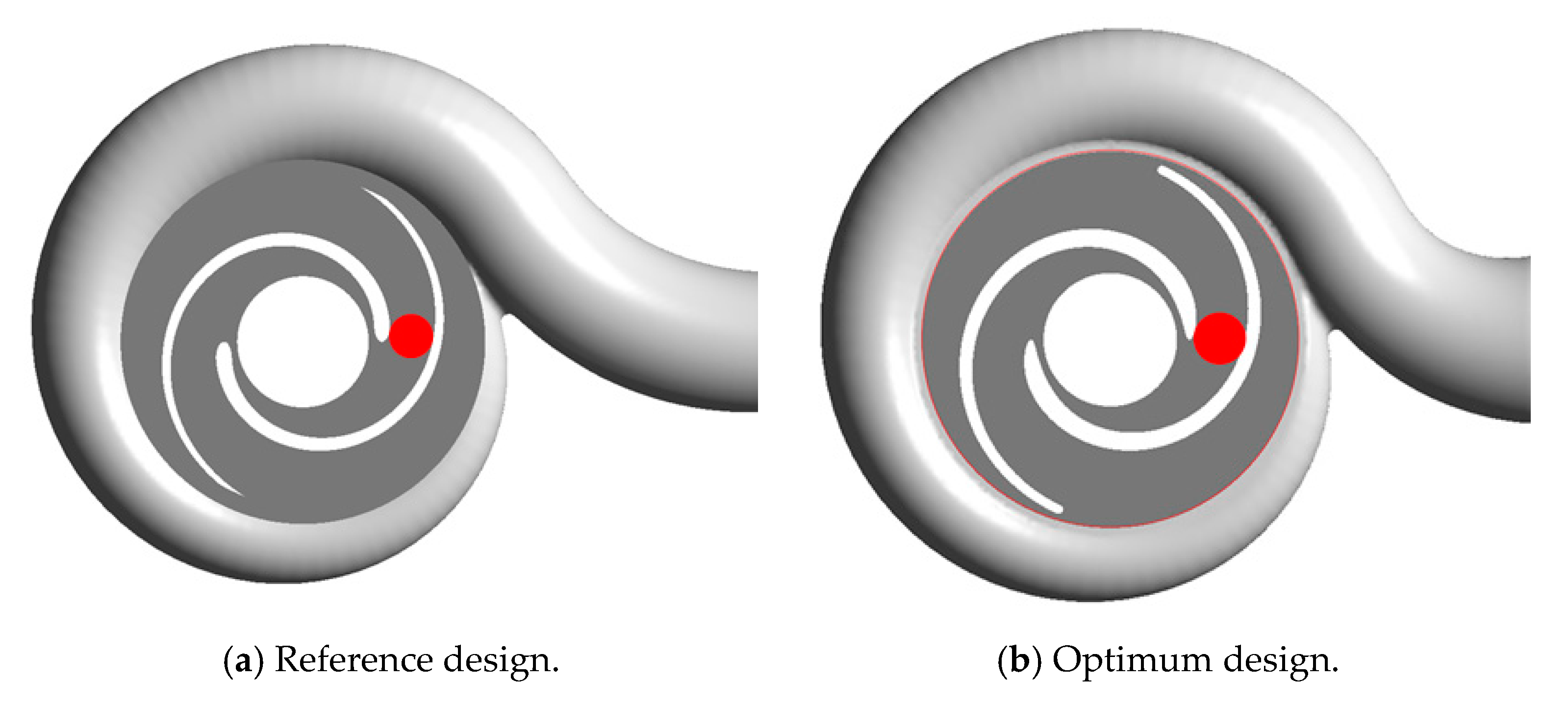
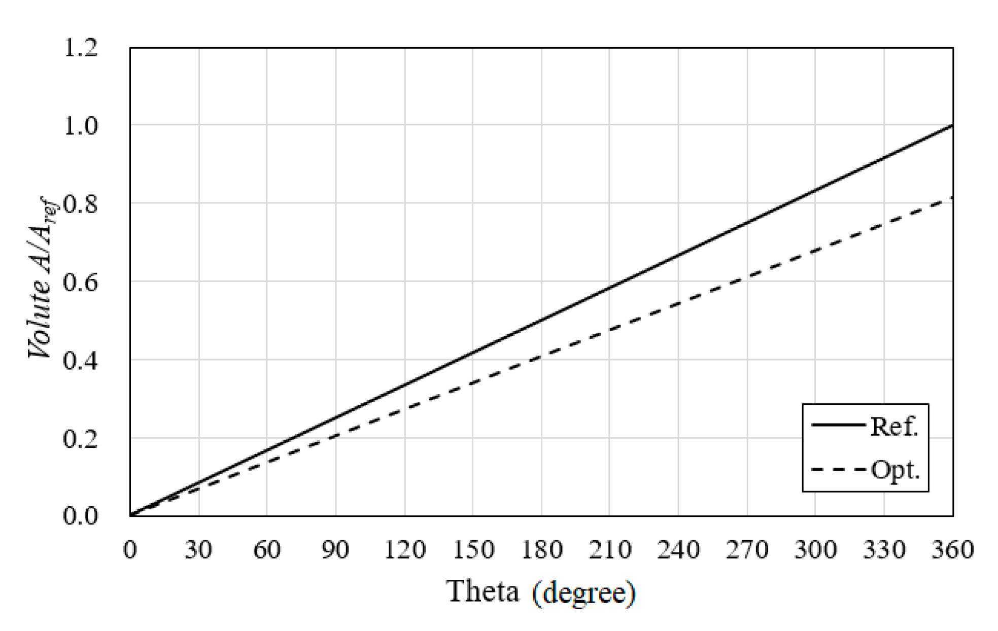
AOD 3, which satisfies the design target, was selected for further analysis of the optimum design. The 3D geometry for AOD 3 is shown in Figure 15. Through optimization, an inlet blade angle of about 1.289 times the reference design and an outlet blade angle of about 0.128 times the reference design were realized. That is, considering the change in the flow path inside the impeller, the blade wrap angle was reduced compared to the reference design. Reduction in the blade wrap angle led to a shorter flow path, thus reducing the friction loss. In the case of the volute, the cross-sectional area of the optimum design was less than that in the reference design. 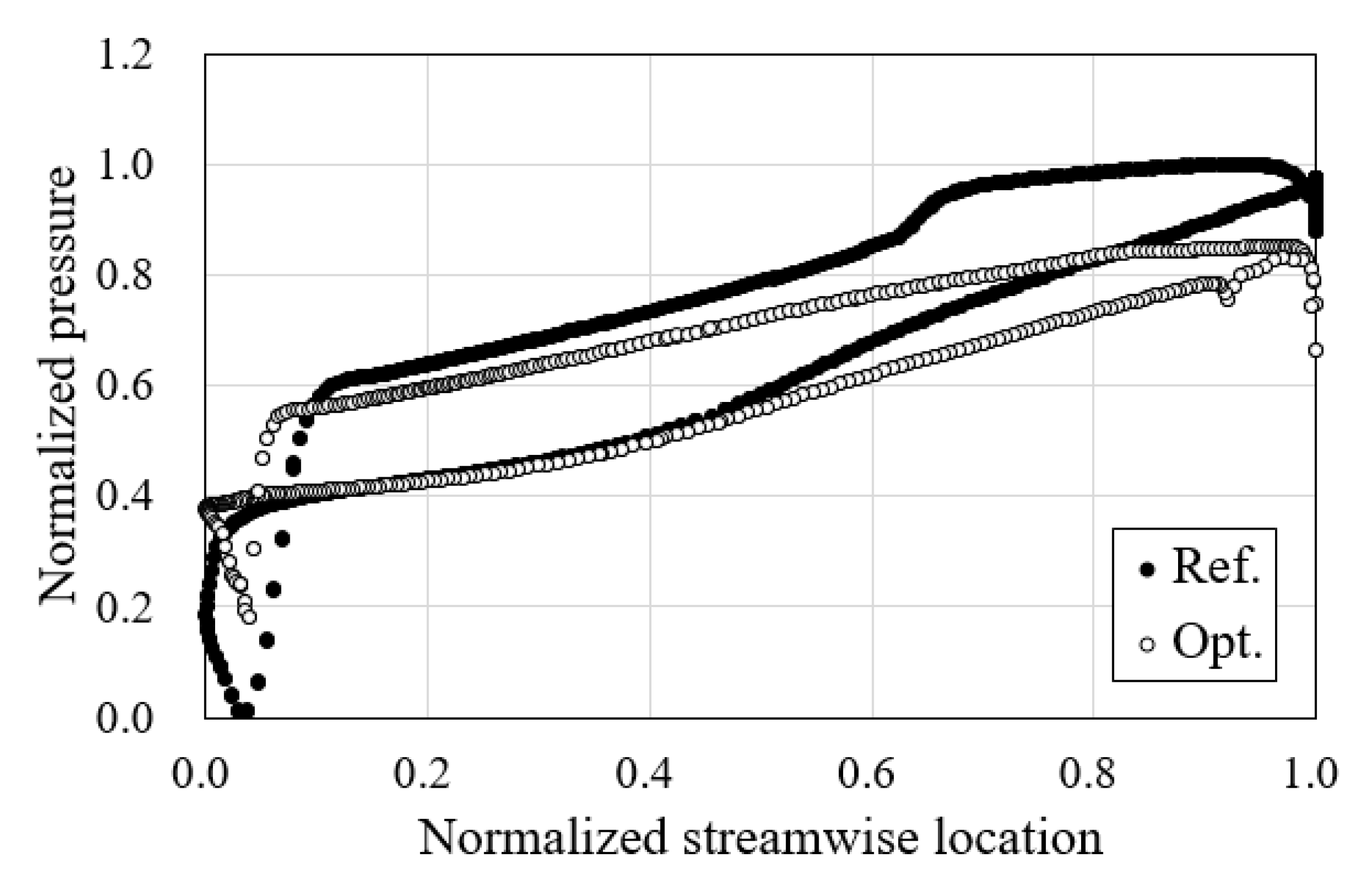Furthermore, the cross-sectional area continuously decreased from the tongue to the outlet, and then it decreased by approximately 18.9% at the outlet, as shown in Figure 16.

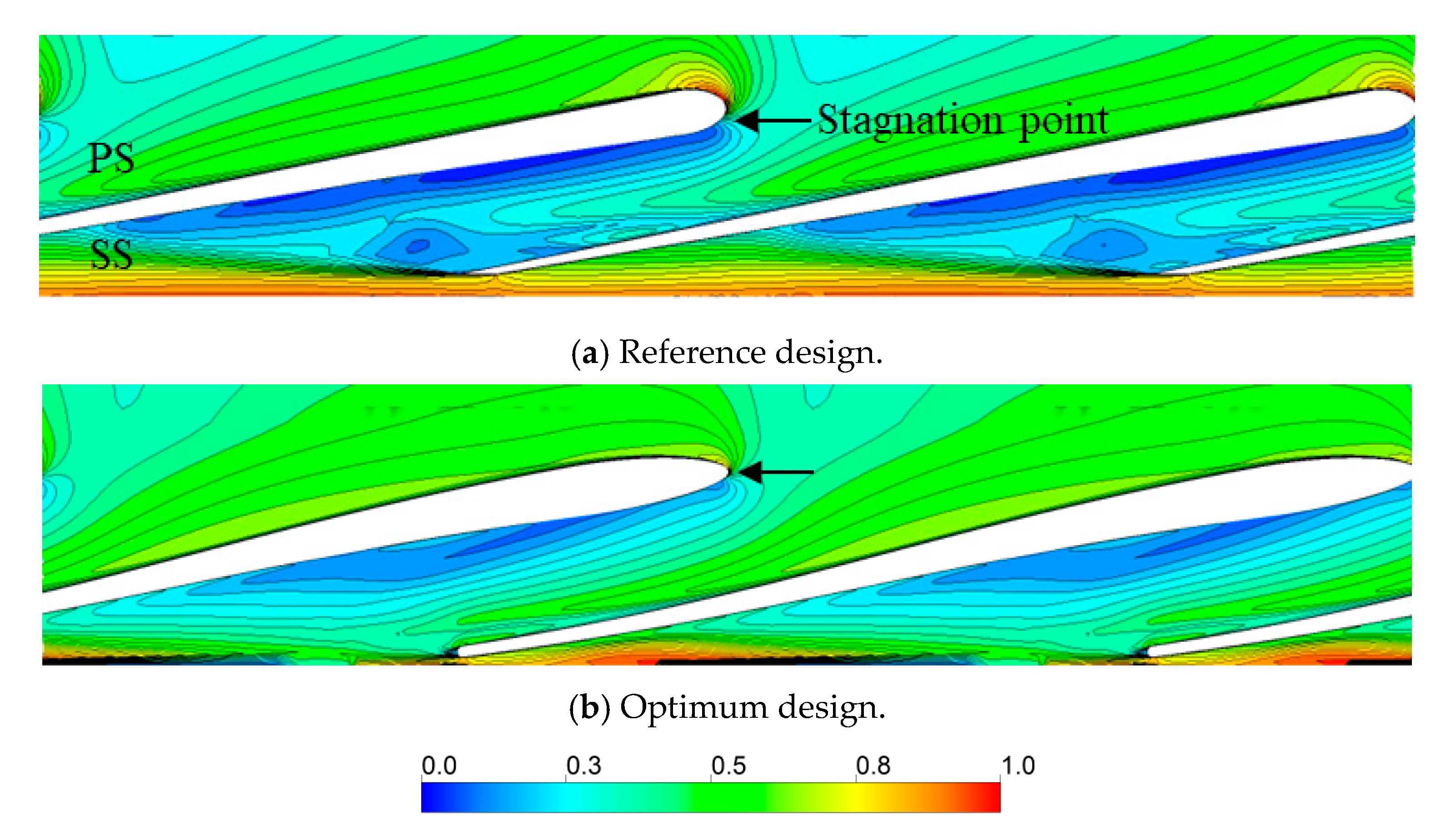
Figure 17 shows the velocity distribution at 50% span of the blade. In the optimum design, the stagnation point is formed at the leading edge of the blade, whereas in the reference design, it is located relatively downstream. This phenomenon occurs because the inlet angle of the blade is not designed to fit the operating condition, and it can increase the incidence angle to cause flow separation and reduce the hydraulic performance of the pump. In addition, the stagnation point is formed on the suction side (SS) of the blade, and the flow proceeds non-uniformly. In particular, a very high-velocity region is distributed at the leading edge (LE) of the pressure side (PS), and severe flow separation occurs at the SS, resulting in a blockage inside the passage.

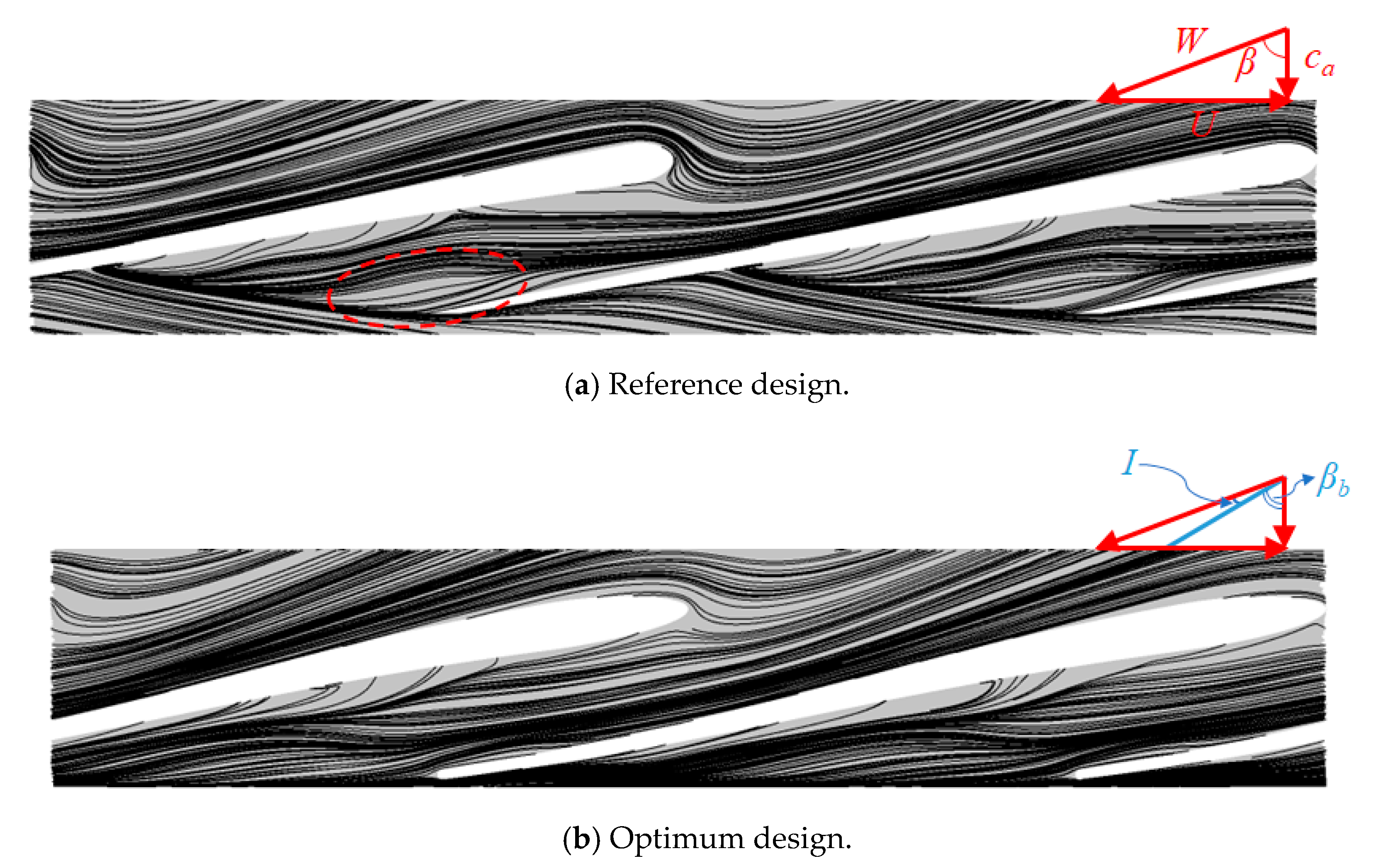
The distribution of the streamlines and the inlet velocity component at 50% span are analyzed and shown in Figure 18. As described in Figure 17, the inlet flow collides at the SS of the blade in the case of the reference design; conversely, in the optimum design, the inlet flow collides precisely with the LE of the blade. Through the optimization, the blade inlet angle (β_b) of the optimum design is greater than that in the reference design, and, therefore, the inlet flow proceeds smoothly, as shown in Figure 17b.

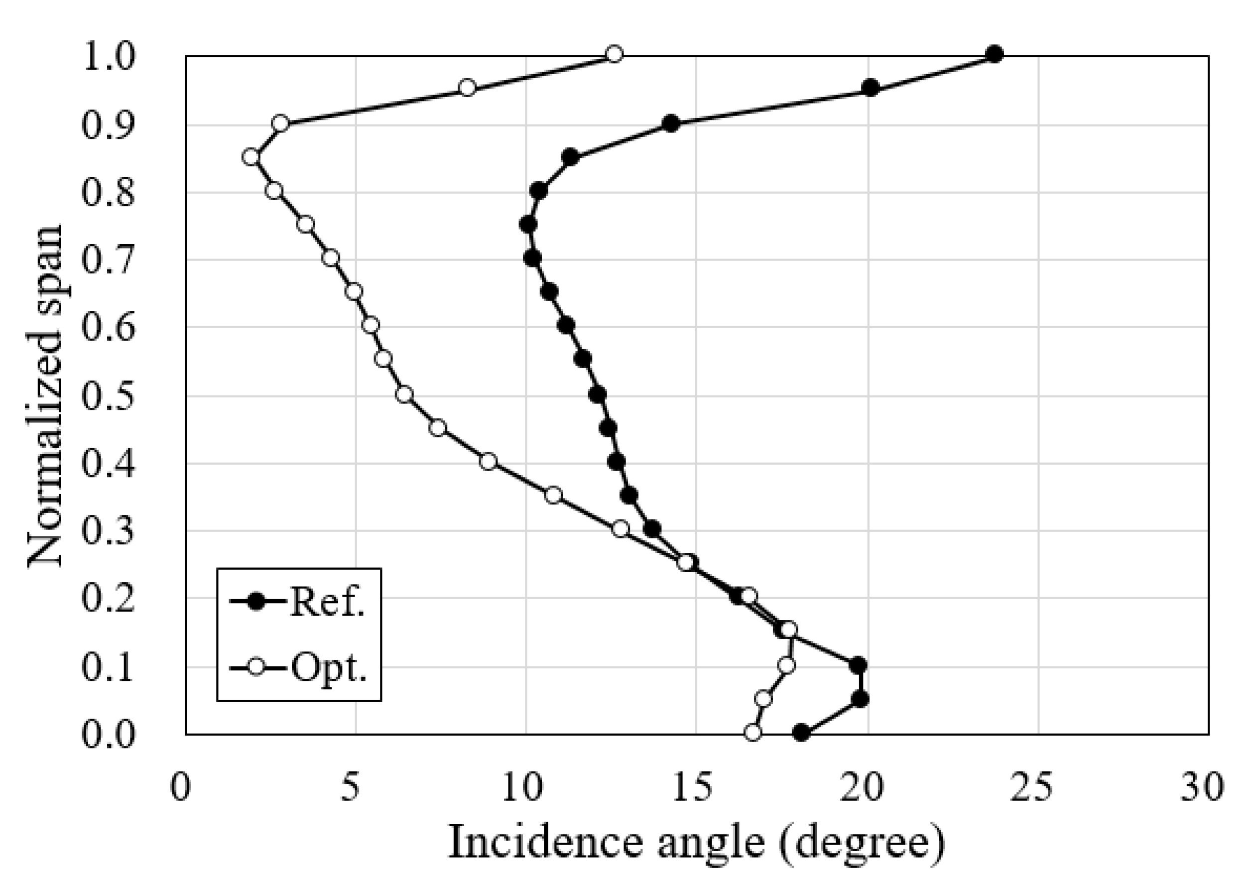
The rotational velocity (U) of the blade, the axial velocity (C_a), and the relative velocity (W) of the flow at the inlet of the impeller can be represented in the velocity triangle diagram. When the three velocity components are known, the flow angle (β) can be derived, and the incidence angle (I) can be calculated by comparison with the blade angle (β_b). The incidence angle distribution from the hub to the tip is shown in Figure 19. The incidence angle of the reference design gradually decreases from the hub to about 80% span and then increases again to the tip span. The tendency of the optimum model is similar to that of the reference design, but the incidence angle is small overall in all spans, compared with the reference design. The largest incidence angle in the reference design is 24° at the tip region, whereas that in the optimum design is 18° at 15% span.

In rotating-fluid machines, the flow is driven by the centrifugal force. Hence, the incidence angle at the tip region is smaller than that at the hub; this improves the hydraulic performance. In particular, since the pump used in this study is a special pump for transporting wastewater, the blade angle distribution from the hub to the tip should be maintained. From this point of view, it is judged that the incidence angle distribution of the optimum design shown in Figure 19 is ideal.

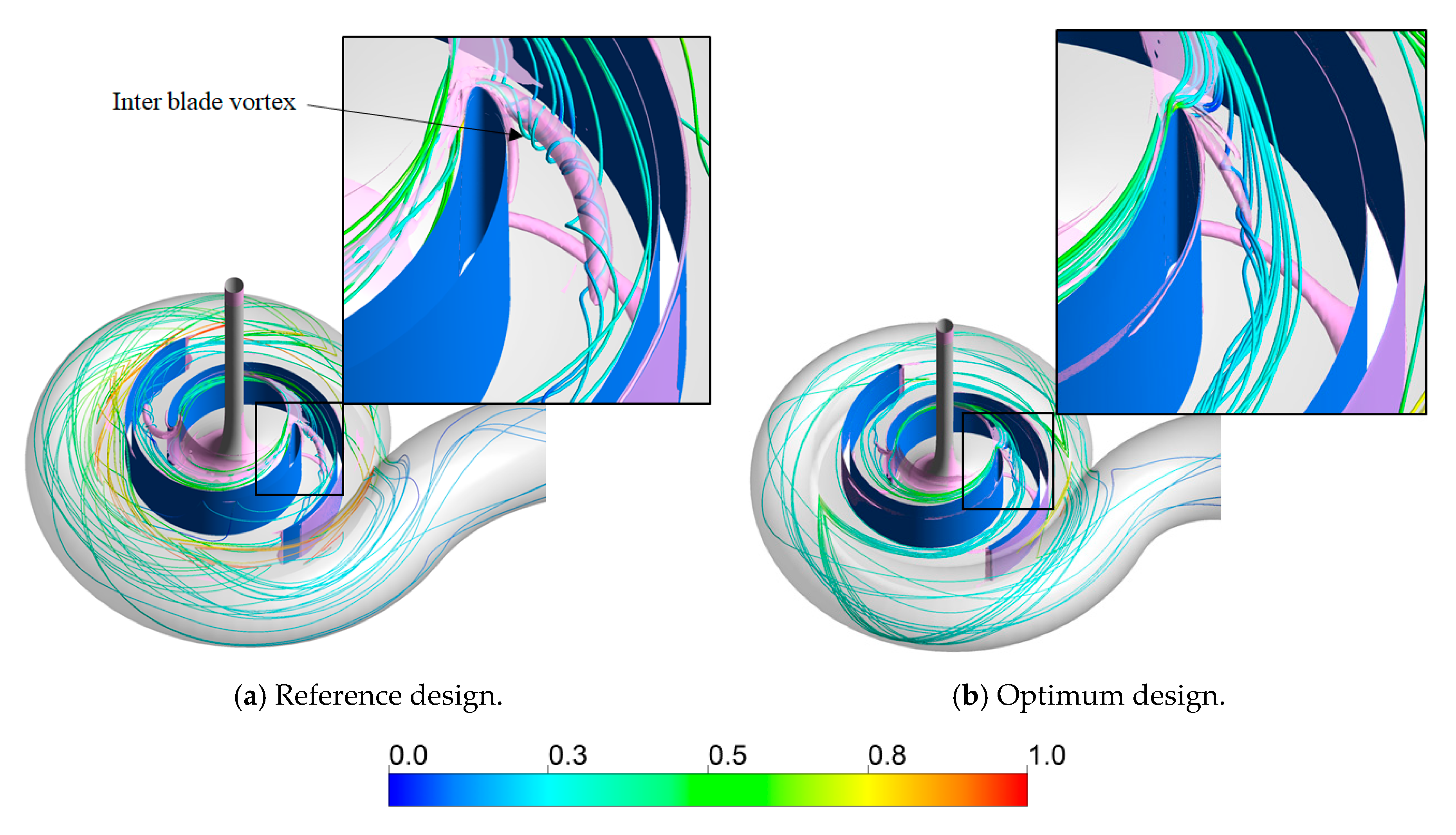
Figure 20 shows the distribution of streamlines and vortices on the iso-surface of the velocity invariant (>5 × 10⁵ s⁻²), to visualize the flow characteristics inside the impeller. As shown in Figure 17 and Figure 18, in the case of the reference design, the inlet flow angle is significantly different from the blade inlet angle, and an apparent inter-blade vortex is observed inside the passage, as shown in Figure 20a. On the other hand, the inlet flow angle of the optimum design agrees well with the blade inlet angle, and the flow proceeds smoothly into the passage, as shown in Figure 20b.

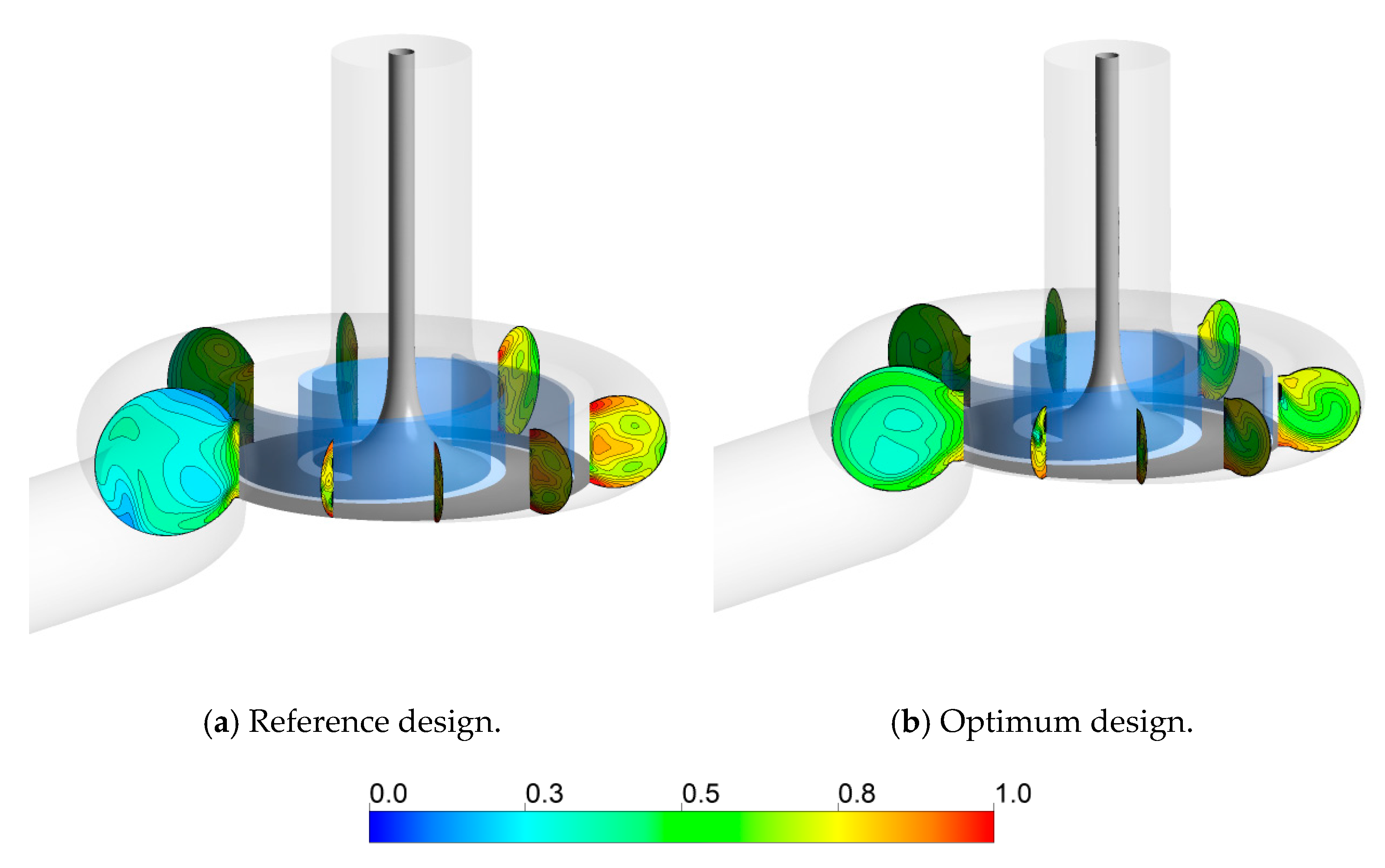
In order to analyze the blade loading, the pressure distribution on the blade in the optimum and reference design are compared, as shown in Figure 21. The pressure values are normalized by using the maximum pressure value of the reference design. Similar to Figure 17 and Figure 18, Figure 21 shows that the static pressure of the reference design at LE is relatively less than that in the optimal design, owing to the rapid increase in the velocity in the PS of the blade LE. In addition, the pressure on the PS and SS of the reference design shows a larger overall region than in the optimum design; in other words, the blade loading of the reference design is larger.

Figure 22 shows the internal velocity distribution from the volute tongue to the outlet. In the reference design, a relatively high-velocity region is distributed near the tongue, but the velocity decreases toward the outlet. On the other hand, the optimum design shows a relatively uniform velocity distribution over the entire area of the volute. In the reference design, the cross-sectional area of the volute is designed to be larger than necessary, and as the flow diffuses near the outlet, it is judged that the static pressure recovery occurs more than in the optimum design.

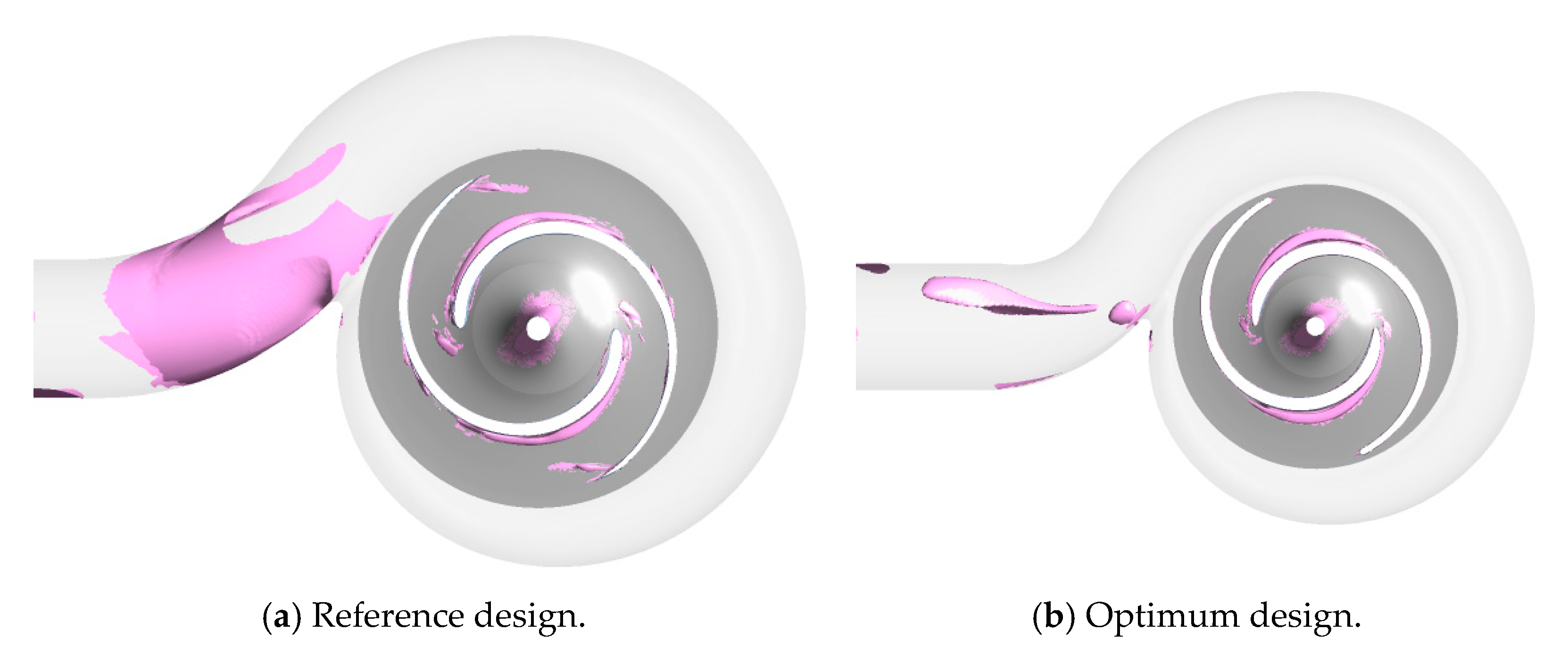
Figure 23 shows the iso-surface contours for a low velocity of 1.0 m/s, to identify the low-velocity region inside the pump. As shown in Figure 22, a relatively wide low-velocity area is formed at the outlet of the reference design. Since the two-vane pump considered in this work is used for transporting wastewater, the solids move inside the impeller and volute. Now, the presence of low-velocity region can cause solids to stagnate. Therefore, the pump should be designed so that no such low-velocity region is created. From this point of view, the optimum design is an ideal design with a significant reduction in the area of the low-velocity region.

6. Conclusions

In the present study, the shapes of a blade and volute were optimized to improve the hydraulic performance of a two-vane pump for transporting wastewater via 3D RANS analysis based on supervised machine-learning optimization. Considering the waste solids, the blade inlet and outlet angles and the cross-sectional area of the volute were selected as the design variables. Three objective functions were considered to maximize the hydraulic performances, i.e., the total head and efficiency of the pump, while maximizing the size of the waste solids.

In this analysis, the RBNN predictive model was trained by using machine learning, and the GA was used to find global optimal solutions. The network training was performed by adjusting the CV error by changing the SC. Through training, an accurate and reliable RBNN surrogate model was constructed, and five arbitrary optimum design points were derived. They were compared with the numerical results to verify the predicted accuracy. The machine-learned surrogate model showed very accurate predictions compared with the numerical results and had relative errors less than 5%.

Through the optimization, the pump was made compact, and the efficiency was improved by about 14% compared to the reference design, while satisfying the design goal of the total head (>10 m). As the cross-sectional area of the optimum volute was reduced, excessive diffusion at the outlet was reduced, and, therefore, the velocity distribution inside the volute was more uniform compared with the reference design. In addition, as the inlet angle of the optimum blade increased, the water flowing from the impeller inlet proceeded smoothly into the flow path, and the flow separation and formation of the inter-blade vortex were significantly reduced.

In future work, the hydraulic performances of the optimum design will be investigated in more detail experimentally, and the characteristics of the flow, containing solid wastes, will be also analyzed.