Article

Drag Effect of Carbon Emissions on the Urbanisation Process: Evidence from China’s Province Panel Data

1
Hospitality Management School, Shanghai Business School, Shanghai 201400, China
2
School of Economics and Management, Tongji University, Shanghai 200092, China
3
Department of Building and Real Estate, Hong Kong Polytechnic University, Hung Hom, Kowloon, Hong Kong 999077, China
4
Land Satellite Remote Sensing Application Center, Ministry of Natural Resources, Beijing 100048, China
*
Authors to whom correspondence should be addressed.
Processes 2020, 8(9), 1171; https://doi.org/10.3390/pr8091171
Submission received: 24 August 2020 / Revised: 13 September 2020 / Accepted: 14 September 2020 / Published: 17 September 2020
(This article belongs to the Special Issue Carbon Capture and Utilisation)

Abstract

:
This study attempts to measure the drag effect of carbon emissions on China’s economic growth by incorporating carbon emissions as an endogenous variable into an economic growth model and by relaxing the assumption that the size of the economy will remain unchanged. The drag effect of carbon emissions on the process of urbanisation is derived based on the intrinsic relationship between economic growth and urban development. Then, unit root and cointegration tests are performed using panel data from 30 provincial regions in Mainland China from 2003 to 2016 to prove and estimate the resistance caused by carbon emission in the process of urbanisation. Results show that the drag effect of carbon emission between 2003 and 2016 has a certain negative impact on the process of urbanisation in China. Due to the constraints of carbon emissions, the growth rate of China’s economic growth and urbanization level is 0.74% and 4.96% lower than that without constraints, respectively. Therefore, in the process of rapid urbanisation, formulating a reasonable carbon emission reduction strategy by the provincial government is conducive to the healthy and sustainable development of urbanisation.

1. Introduction

In most cases, a socioeconomic system is considered an evolving subsystem in the ecosystem. In comparison with independent systems, socioeconomic systems require unlimited inputs and outputs [1]. Romer noted that socio-economic development required attention to the interdependence with nature. He believed that any attempt to seek unlimited growth in output will eventually run out of resources and fail [2]. Similarly, the limited supply of natural resources (land) may impose implicit constraints on productive capacity [3]. While energy and materials are now widely recognised as essential for industrial activities, natural resources and natural resource-based industrialisation are considered to be part of social growth and development, which previous studies have provided valuable theoretical support [4,5,6]. Romer defined the drag effect of natural resources on economic growth (Because of the limitation of resources, the consumption of resources in the last stage will inevitably lead to the reduction of input of economic output in the next stage. This phenomenon is called “growth drag.) and constructed a neoclassical model to derive the basic structural parameters of the growth drag [2]. Nordhaus also had additional policy discussions on this issue [4]. By using the model constructed by the Romer and using the statistical data from 1981 to 2002, Xie et al., studied the growth drag effect on economic of water resources and land resources in China [7]. The results showed that the drag effect of water resources was 0.001397 and that of land resources was 0.013201. On the basis of Romer’s growth drag theory, Li and Shen [8] quantified the energy structural constraints on China’s economic growth by relaxing its assumption that the size of the economy will remain unchanged. From the point of view of hindering economic growth, the results showed that the main energy has a significant binding effect on economic growth. From the provincial level, Xie and Mu [9] explored the constraint mechanism of energy growth drag and studied the influence factors of energy growth drag in China’s economic development. Most of the aforementioned studies explored the growth drag of non-renewable resources on economic development from the application level.
The limitation of previous studies on growth drag is that most them mainly focus on economic production and analyze by using time series data. This limitation leads to two challenges. The first is that many studies may omit variables to cause deviations. For example, production functions usually ignore or underestimate the impact of environmental pollution resistance. The second limitation is that these studies usually cannot avoid low efficacy problems related to traditional unit root test and cointegration test. The problems of these methods will undoubtedly hinder the development of many early studies. Therefore, the drag effect of economic growth must be investigated from a new perspective.
Urbanisation is an the inevitable result of the economic and social development of a country or region, and in a certain sense, its degree of development represents the level of development of a country or region [10]. For 40 years (1978–2018), China’s economic and social development has made remarkable achievements. China’s urbanisation rate rose from 10.6% in 1949 to 59.6% at the end of 2018 [11], and the resident population of towns and cities has increased by more than 500 million. As an important driver of China’s economic growth, urbanisation’s net contribution to China’s economic growth has reached more than 3.6% [12].
However, it is constrained and restricted by various non-renewable resources in the process of urbanisation. Analysing the drag effect of resource consumption in China’s urbanisation process, Liu and Chen [13] found that the urbanisation drag values of energy, land and water resources are 0.00848989, 0.00028236, and 0.015188131, respectively, and the sum of these drag effects on economic growth is 0.023889489. Wang and Chu [14] constructed a drag effect model of energy consumption in the process of urbanisation based on the urbanisation growth function, and analysed the drag effect of Liaoning Province quantitatively. The results showed that energy constraint has a significant drag effect on the urbanisation process in Liaoning Province. Many scholars have studied the impact of carbon emissions on urbanisation development from the aspects of urban migrants [14,15,16], ecological environments [17,18,19], and urban competitiveness [20]; however, the direct constraints of carbon emissions on urbanisation development are rarely studied.
Even though existing research has shown that carbon emission constraint has become an important bottleneck in economic growth, the drag effect of resource consumption in China’s urbanisation process from a constraint perspective is also rarely investigated. Rapid urbanisation leads to the shortage of resources and the deterioration of environmental pollution [21]. In order to effectively solve environmental problems, the Chinese government has proposed measures (such as reducing carbon emissions) to speed up environmental protection and build ecological civilization [22]. China’s government calls for attention to the quality of urban development, promoting low-carbon development, and adopting a low-carbon lifestyle and urban construction model [18], which attracted the attention of local governments and research scholars [23]. Therefore, this paper intends to use the model of drag effect of carbon emission on the process of urbanisation to calculate the resistance by carbon emission to urbanisation. According to the conclusion of the study, the policy suggestions are given for the low carbon urbanisation in the stage of rapid development, which is conducive to the healthy and sustainable urban development.
The present work integrates carbon emissions as an endogenous variable into an economic growth model, relaxes its assumption severing the same about the size of the economy, examines the unit root and cointegration relationship by using panel data, and then measures the carbon emission constraints of China’s economic growth. This method allows the sample to be interpreted with a high degree of freedom to perform accurate and reliable statistical testing. At the same time, the use of panel cointegration test can reduce the collinearity among regression variables, thereby allowing heterogeneity across regions. Finally, the drag effect of carbon emission on the process of urbanisation is derived based on the intrinsic relationship between economic growth and urbanization (Carbon emissions are regarded as a limited, non-growth system, which establishes the constraint of carbon emissions on economic growth. There is a close relationship between economic growth and urbanisation in China at the present stage, and then the drag effect of carbon emission on the process of urbanisation is deduced. More details can be seen in Section 3.2).

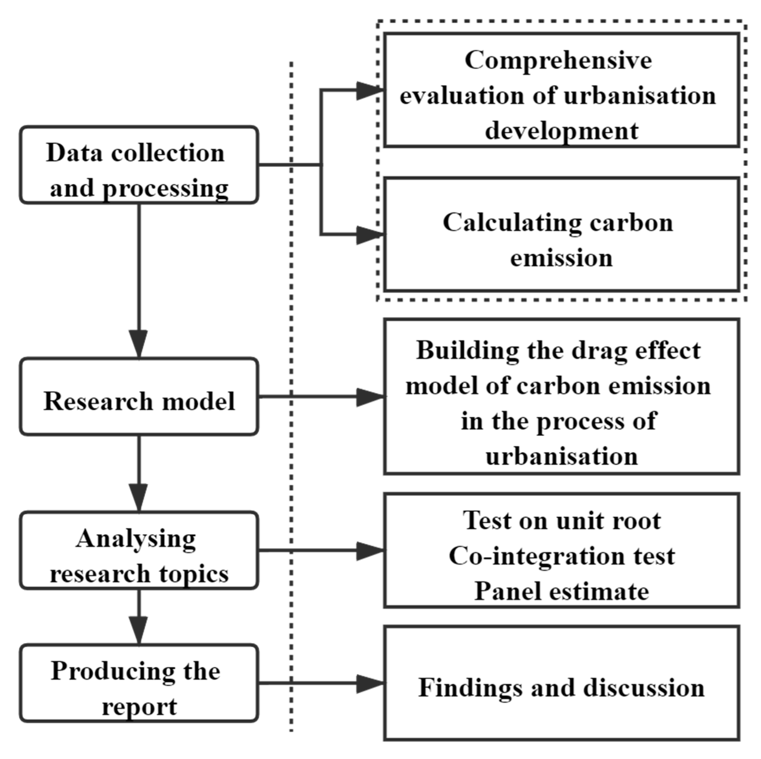
2. Data Collection and Processing

In 2003, the Chinese government proposed a ‘people-oriented, comprehensive, coordinated and sustainable scientific concept of development’; since, ecological and environmental issues concerning China’s economic and social development have been paid increasing attention. The time interval for this study is set for 2003–2016, and the study targets are 30 provincial administrative regions in Mainland China. In this manner, the scientific, accurate and practical feasibility of China’s urbanisation development of the drag effect of carbon emission can be studied. The main source of the data is from the statistical yearbook from 2003 to 2016, and some individual data must be calculated. The main references include the Yearbook of China Statistics, the Yearbook of China’s Urban Statistics, the Yearbook of China’s Urban Construction Statistics and the Yearbook of China’s Energy Statistics, which can be got on the website of the National Bureau of Statistics of China [11].
According to the Intergovernmental Panel on Climate Change (IPCC) report, fossil fuel combustion is a major source of carbon in the atmosphere and a major cause of global climate change and greenhouse effect [24]. As a gathering place for global population and economic activity, cities, emitting both direct and indirect CO2 emissions, account for the absolute body of global emissions [25,26,27]. Satterthwaite’s research suggests that cities are regions where human activities have the deepest impact on the surface, with concentrated fossil fuel combustion and more than 80% of CO2 emissions generated from urban areas [26]. The present work uses the IPCC guidelines [24] to recommend a uniform standard methodology for calculating CO2 emissions from cities with available energy consumptions. The types of energy considered are raw coal, coke, crude oil, gasoline, kerosene, diesel, fuel oil, natural gas, heat and electricity, as shown in Table 1.
An estimate of the K value is required because no data are available on the fixed capital stock (K) for the calendar year in the statistical yearbook. For the calculation of K value, the perpetual inventory method [28] is widely used. In specific accounting, scholars have used the information they have obtained as a basis, and have considered various methods. For example, He [29] measured China’s existing productive and unproductive assets for 1920–1990 on the basis of existing productive accumulation and non-productive indices. Ye [30] used another method of capital measurement to calculate the total factor productivity throughout the country and specifically, in its provinces and districts. For simplicity, this study intends to use Zhang’s calculation method This approach carefully calculates and accounts the initial capital value for each province in 1978 as the benchmark capital stock, and it will not be listed separately in this paper.
The research areas and data sources are introduced as follows. Firstly, the data collected area calculated to arrive at a comprehensive assessment of urban development and carbon emissions. Then, the drag effect model of carbon emission on urbanisation is derived by using an economic development growth drag model. Subsequently, through unit root and cointegration tests, nonlinear partial least square (PLS) method is selected to obtain the carbon emission drag effect of urbanisation development at the provincial level in China, as shown in Figure 1.

3. Methods

In this part, it mainly introduces the method of measuring the level of urbanisation, then establishes the drag effect model of carbon emission in the process of urbanisation, finally carries on the empirical analysis using the unit root test and the cointegration test.

3.1. Comprehensive Measurement Model of Urbanisation Level

The targets of this study include 30 provincial administrative regions (i.e., Beijing, Shanghai, Tianjin, Chongqing, Inner Mongolia, Xinjiang, Ningxia, Guangxi, Heilongjiang, Jilin, Liaoning, Hebei, Henan, Shandong, Shanxi, Hunan, Hubei, Anhui, Jiangsu, Zhejiang, Fujian, Jiangxi, Guangdong, Hainan, Guizhou, Yunnan, Sichuan, Shaanxi, Qinghai and Gansu). These provincial districts are classified into the northeast, eastern coast, central and western regions of China, as shown in Figure 2.
The earliest literature on the development of urbanisation can be traced back to Marshall in 1890 and Jacobs in 1969 [31,32]. These authors were the first to propose the theory of external economies of scale to explain the formation and development of cities. External economies of scale can be divided into localised economies (industrial externalities) and urbanised economies (concentrated economies) to promote the transfer of enterprises and labour to cities, which are attracted by micromechanisms and external economies of scale, respectively.
Many scholars have also made empirical studies on the determinants of urbanisation development. For example, Jacobs [32,33], Pirenne [34], Polanyi [35], Pandey [36] and Chandler and Fox [37], among others, have highlighted these processes. From these works to the present, there is a large amount of theoretical and empirical literature on the factors that affect the urbanisation process. These literatures verify the correlation between industrialization level, trade, transportation, wage level and urbanisation development, but do not explain the causal relationship between urbanisation development and these factors. The same problem exists in Chang and Brada’s [38] study of China’s urbanisation rate. Research on the influence factors of urbanisation in China also has such problems [39,40,41].
Cities are the most important region for CO2 generation and are the core regions for reducing CO2 emissions in China. The development of urbanisation has changed the form of urban space and people’s way of life and increased energy consumption, which are the main factors that affect CO2 emission. Urbanisation is a complex socialisation process. Thus, on the basis of analysing the impact of urbanisation on carbon emission, this study establishes an index system to comprehensively measure urbanisation development.
Incorporating existing research on the influencing factors of urbanisation [42,43,44], this study intends to comprehensively measure the development of urbanization. While conforming to the people-oriented, quality-critical urbanisation requirements, this study also strives to take into consideration an overarching aim: to sort out the relationship between urbanisation development and carbon emissions [45]. The comprehensive measurement index system of urbanisation measures the development level of urbanisation from the three dimensions: scale, structure, and technology. On the basis of the connotation of urbanisation, research results of previous studies [39,40,46,47,48] are used as reference, with the indicators shown in Table 2 to describe the level of urbanisation. The level of urbanisation is measured by adopting the entropy weight method (Appendix A).
As shown in Table 2, the scale dimension of measuring the level of urbanisation is characterised by economic and population qualities. Economic quality is expressed in terms of Gross Domestic Product (GDP) per capita (10,000 yuan/person) and economic growth (%). GDP per capita (10,000 yuan per person) describes the level of economic development. The mode of economic growth (%) is expressed as a proportion of GDP in fixed assets and describes economic vitality. These two characterise the quality of the economy. The level of education (10,000) and the proportion of the labour force in the total population (%) reflect the population quality.
The structural dimension of the level of urbanisation is measured from the economic and land use structures. The proportion of non-agricultural industry characterised by the second and third industries in GDP (%) describes the condition of industrial transfer. Land use structure is characterised by land use intensity and land input intensity. Land use intensity (%) indicates the scale of urban development, while land input intensity (%) describes the intensity of urban development.
The technical dimension of the level of urbanisation is measured from three aspects, namely, external communication, scientific research strength and environmental governance ability. Foreign direct investment in external communication (10,000 yuan) indicates the external environment of technological upgrading. The scientific research strength is described by the per capita scientific research input (10,000 yuan/person), which expresses the material guarantee of technological progress. A city’s environmental governance capacity is closely related to the level of technology, which is reflected by environmental regulation intensity (10,000 yuan/km2).

3.2. Drag Effect Model of Carbon Emission in the Process of Urbanisation

Figure 3 shows the drag effect relationship between urbanisation development and carbon emissions. This relationship establishes a link to economic growth by using carbon emissions as the most direct output for resource. At present, China’s urbanisation development and economic growth have a close relationship and mutual promotion. Through the middle factor of economic growth, the relationship between carbon emissions and urbanisation development is established.
Sustainable development theory holds that natural resources, ecological imbalances, pollution and other environmental factors play a crucial role in the long-term sustained growth of the economy. The pursuit of an economic model of permanent output is infeasible due to limited resources, and although economists have made many revisions and explorations of economic models from a ‘scarcity’ perspective, most of them do not effectively incorporate resources into their models.
On the basis of a large number of neoclassical economic theories, Romer [2] proposed a model of economic growth under resource constraints by using the Cobb-Douglas function to make it more operable. In addition, the factors are assumed to pay their marginal products [49,50]:
Y ( t ) = K ( t ) α R ( t ) β T ( t ) ε [ A ( t ) L ( t ) ] 1 α β ε ( α > 0 , β > 0 , γ > 0 , α + β + γ < 1 )
where Y ( t ) , K ( t ) , L ( t ) and A ( t ) represent the output, capital, labour and knowledge or the effectiveness of labour, respectively; R ( t ) refers to the natural resources available in production; T ( t ) represents the amount of land; α refers to the elasticity of capital production; β refers to the elasticity of resource production; ε is the elasticity of land production; and t represents time. This model sets the same capital and scale of labour compensation.
By applying this primitive model, the optimal growth theory can be derived from the binding effect of energy on economic growth. The energy elements are added to Solow’s [51] classic model, and the model is expanded as follows:
Y ( t ) = K ( t ) α E ( t ) β [ A ( t ) L ( t ) ] γ , ( α > 0 , β > 0 , γ > 0 , α + β + γ < 1 )
where Y ( t ) , K ( t ) , L ( t ) and A ( t ) represent the output, resource, labour and knowledge or the effectiveness of labour, respectively; E ( t ) refers to the natural resources available in production; α refers to the elasticity of capital production; β refers to the elasticity of resource production; γ is the elasticity of labour-related production; and t denotes time. This model sets the same capital and the scale of the labour compensation.
As shown in previous studies, China’s urban carbon emissions are comprised mainly of energy use. According to [52] as well as [53], the assumption that relax the size of the economy will remain unchanged, and a model of the drag effect of carbon emissions on economic growth can be obtained as follows:
Y ( t ) = K ( t ) α C ( t ) β [ A ( t ) L ( t ) ] γ , ( α > 0 , β > 0 , γ > 0 , α + β + γ < 1 )
where Y ( t ) , C ( t ) , L ( t ) and A ( t ) represent the output, carbon emission, labour and a combination of ‘knowledge’ or ‘effectiveness of labour’ that indicates effective labour; C ( t ) represents the carbon emissions in production; α refers to the elasticity of capital production; β refers to the production elasticity of carbon emissions; γ is the elasticity of labour-related production; and t represents time. The dynamics of capital, labour and labour effectiveness are consistent with the classic Solow model, as shown as follows:
K ( t ) = s Y ( t ) δ K ( t )
L ( t ) = n L ( t )
A ( t ) = f A ( t )
where s refers to the saving rate, δ refers to the depreciation rate of capital, n represents the labour growth rate and f represents the technology growth rate. Here, the carbon capacity systems are limited and non-growing [53]. Therefore, human economic behaviour must be coordinated with the constraining characteristics of the carbon capacity system. Economic growth should also be balanced with carbon capacity, most directly resulting in the gradual reduction of carbon emissions.
Therefore, this study makes the following assumption:
C ( t ) = b C ( t )
where b represents the growth rate of carbon emission, and b > 0. Following the previous assumptions, A, L, and C all grow at constant rates. K and Y also maintain constant growth rate under balanced growth path dependency. The growth rate K is developed from Equation (4), as shown as follows:
K ( t ) K ( t ) = s Y ( t ) K ( t ) δ
From Equation (8), one of the necessary conditions to keep the growth rate K constant is to maintain Y K unchanged. Thus, the growth rate of Y and K is equal, which is expressed by g Y = g K .
Then, logarithm of Equation (3) is taken as follows:
ln Y ( t ) = α lnK ( t ) + β ln C ( t ) + γ [ ln A ( t ) + ln L ( t ) ]
By taking the derivative of Equation (9) with respect to time t, the relationship between the growth rates of each variable is obtained as follows:
g Y ( t ) = α g K ( t ) + β g C ( t ) + γ [ g A ( t ) + g L ( t ) ]
where g ( t ) represents the growth rate of each corresponding variables. Previously, A, L and C growth rates are set to f , n and b , respectively. Then, Equation (10) can be simplified as follows:
g Y ( t ) = α g K ( t ) β b + γ ( f + n )
The balanced path g Y = g K yields:
g Y * = γ ( f + n ) β b 1 α
where g Y * represents the growth rate of the output on the balance path. The growth rate of average output per unit of labour under the balanced path can be expressed as follows:
g Y / L * = g Y * g L * = γ ( f + n ) β b 1 α n = f γ + n γ + n α β b n 1 α
The calculation can be derived in Equation (13) that the driving force of technological progress on the average growth rate of output per unit of labour, γ f 1 α , belongs to the forward or positive driver. The drive rate of the growth rate of labour to per capita output is n ( γ + α 1 ) 1 α , which may be a positive or negative driver. Carbon emissions hinder the growth in average labour output. The greater the carbon emission growth rate b is, the smaller the value of g Y / L * . That is, carbon emissions are more constrained to economic growth. Therefore, whether g Y / L * is negative or positive cannot be determined under the assumption of balanced growth. When g Y / L * is negative, carbon emissions are negative drivers of economic development instead of growth drivers of technological progress. The drag effect of economic growth is that the economic development is a high-consumption and high-emission model. The opposite is true when g Y / L * is positive.
Assume that carbon emissions are unconstrained, and their growth is in accordance with that of the labour force. Then, Δ L ( t ) = n C ( t ) . By applying Equation (12), the growth rate of average output per unit of labour in the context of balanced economic growth can be expressed as follows:
g Y / L * ˜ = f γ + n γ + n α + β n n 1 α
The drag effect of the growth of carbon emission constraints is the difference between the growth rate of average output per unit of labour and the growth rate under carbon emission constraints in the context of economic balance.
D r a g C Y = g Y / L * ˜ g Y / L * = f γ + n γ + n α + β n n 1 α f γ + n γ + n α β b n 1 α = β ( n + b ) 1 α
Equation (15) shows that the drag effect of economic growth under carbon emission constraints is positively correlated with the output elasticity of carbon emissions β , the growth rate of labour force n , and the elasticity of capital output α . The economic implication is that if growth depends on high carbon emissions rather than technological progress, then growth will eventually slow down. Disordered and blind investment of capital and labour also increases drag effects. When b is positive, the drag effect is greater. That is, the faster the growth rate of carbon emissions is, the greater the resistance to economic growth will be, indicating that extensive economic growth is unsustainable. This finding is also in line with the realistic development requirements of eliminating high-energy consumption and high emission path.
The drag effect of carbon emission on urbanisation must be derived by the intermediate variable of economic growth. Zhou’s [54] research holds that the effect of economic growth on urbanisation is greater than that of urbanisation, and a half-positive curve relationship exists between the two. Therefore, the relationship of the two can be described as follows:
U ( t ) = c + d L n Y ( t ) + ε
where U represents the urbanisation level, and D is the elasticity coefficient for the level of urbanisation for economic growth. The index is calculated, and the derivative of Equation (16) is shown as follows:
Δ U ( t ) = d g Y ( t )
where Δ U represents the annual rate of urbanisation. On the basis of the above derivation process, the drag effect of carbon emission on urbanisation can be described as follows:
D r a g C U = d D r a g C Y = g U / L * ˜ g U / L * = d β ( n + b ) 1 α
By analysing Equation (18), the elasticity coefficient of economic growth on urbanisation d also has an impact on the drag effect of urbanisation under the carbon emission constraint. If d is positive, then the drag effect of carbon emissions on urbanisation and the drag effect of economic growth are the same. On the basis of the existing research literature and related statistics, China’s urbanisation development and carbon emissions are positively correlated [43,55,56]. Therefore, the drag effect here should also be positive. The results will be validated in the empirical part.

3.3. Test on Panel Unit Root

Recent developments in the literature suggest that panel-based unit root tests have higher power than unit root tests based on individual time series. Newly developed panel unit root tests include those of Breitung [57]; Hadri [58]; Levin et al., [59]; and Im et al., [60]. The following autoregressive model is considered:
y i t = ρ i y i t + δ i X i t + ε i t
where i = 1, 2, …, N represents the ith province observed over periods t = 1, 2, …, T; Xit is the exogenous variable in the model, including any fixed effects or individual trend; ρ i is the autoregressive coefficient; and ε i t is a stationary process. If ρ i < 1, then y i is said to be weakly trend-stationary. Conversely, if ρ i = 1 , then y i contains a unit root. The LLC, Breitung and Hadri tests assume that the ε i t are IID (0, ε i t 2 ), and ρ i = ρ for all i. Accordingly, the coefficient of y i t 1 is homogeneous across all cross-sectional units of the panel [61], and individual processes are cross-sectionally independent. Pesaran and Smith (1995) [62] highlighted the importance of parameter heterogeneity in dynamic panel data models and analysed the potentially severe biases that could arise from including it inappropriately.
Thus, this study adopts the IPS test, which allows for a heterogeneous coefficient of y i t 1 . This approach is a more reasonable proposition because heterogeneity can arise from different economic conditions and levels of development in each province [63]. IPS proposes averaging the augmented Dickey–Fuller (ADF) tests, that is, ε i t = j = 1 p i φ i j ε i t j + μ i t while allowing for different orders of serial correlation. Substituting this expression into Equation (19) yields the following:
y i t = ρ i y i t 1 + j = 1 p i φ i j ε i t j + X i j δ i + ε i t
where ρ i is the number of lags in the ADF regression. The null hypothesis is that each series in the panel contains a unit root (i.e., H0: ρ i = 1 for all i). The alternative hypothesis is that at least one of the individual series in the panel is stationary (i.e., H1: ρ i < 1 for at least one i). IPS defines a t-bar statistic as the average of the individual ADF statistic, that is:
t ¯ = 1 N i = 1 N t ρ i
where t ρ i is the individual t-statistic for testing (i.e., H0: ρ i = 1 for all i). The t-bar statistic has been shown to be normally distributed under H0, and the critical values for given values of N and T are provided by the IPS [60].

3.4. Cointegration Test on Panel Data

If the unit root tests establish that the variables are integrated of order one, then the next step is to apply cointegration analysis to determine whether a long-run relationship exists among them. This approach is performed by applying the Pedroni heterogeneous panel cointegration test [64]. Pedroni (2000) provided seven statistics to test the null of no cointegration in heterogeneous panels. One group of tests was termed ‘within dimension’ (panel tests), whereas the other group of tests was ‘between dimension’ (group tests). The within-dimension tests considered common time factors and allowed for heterogeneity across countries. The between-dimension tests were ‘group mean cointegration tests’ and allowed for heterogeneity of parameters across provinces. The seven Pedroni (2000) test statistics can be expressed as follows. (1) Within-dimension panel tests are: (a) panel v-statistic, (b) panel Phillips-Perron-type rho-statistics, (c) panel Phillips-Perron-type t-statistic and (d) panel ADF-type t-statistic. (2) Between-dimension group tests are: (e) group Phillips-Perron-type rho-statistics, (f) group Phillips-Perron-type t-statistic and (g) group ADF type t-statistic. Pedroni’s (2000) seven statistics are based on the estimated residuals from:
Y i t = α i + β i K i t + i L i t + ϑ i C i t + ε i t
where Y i t , K i t , L i t and P i t are the total output, capital inputs, labour inputs and the CO2 flow for the ith province at time t, respectively; and ε i t = η i ε i ( t 1 ) is the estimated residual from the panel regression. The null hypothesis tested is whether η i denotes unity. The finite sample distribution for the seven statistics is tabulated by Pedroni [65] using Monte Carlo simulations. If the test statistic exceeds the critical values in Pedroni, then the null hypothesis of no cointegration is rejected, implying a long-run relationship exists among the variables.

4. Research Analysis

4.1. Test on Unit Root

A non-smooth time series occurs because the statistical laws of panel data often change over time for miscellaneous reasons. ‘Pseudo regression’ may occur if non-smooth time series data are directly regressed. Then, the Gauss-Markov theory is no longer valid, and parameters estimated by ordinary least square (OLS) by use (OLS) are no longer consistent. Therefore, the data stability (unit root) must be tested before the panel data can be regressed. A panel unit root test is conducted before performing the cointegration analysis of the panel data. Three tests, namely, those of LLC, IPS and Breitung, are also performed. In addition, this study follows the procedures of Maddala and Wu [66], who proposed a straightforward, nonparametric unit root test and suggested the use of Fisher-ADF and Fisher-PP statistics. If the panel data have a unit root process (non-smooth data), they must be cointegrated because a set of non-smooth time series does not have a cointegration relationship and goes directly to the model regression. The result will also produce a pseudo regression phenomenon. The logarithmic calculation of the panel data of economic output (Y), labour (L), urban carbon emissions (C) and fixed capital stock (K) are taken as lnY, lnK, lnL and lnC, respectively. Table 3 presents the results of the panel unit root tests.
Table 3 shows that the first-order difference between the three test method variables (i.e., lnY, lnL and lnC) is stable. The first-order difference of lnK in the ADF test method is not smooth. However, taking the second-order differential sequence for all variables is smooth. The lnK p value is 0.000 in the ADF test method, which is at a significant level of 1% to reject the original assumption. Under such test results, the panel data must be cointegrated.

4.2. Cointegration Test

As shown in Table 4, with the exception of panel and group rho-statistic, the other tests reject the ‘no cointegration’ assumption at significant levels of 10%, 5%, and 1%.
Thus, China’s economic development and carbon emission endogenous growth model meets the requirements of the panel common model. Moreover, a long-term equilibrium relationship exists between economic growth and economic factors. That is, a cointegration relationship exists between the non-stable time series lnY and lnL, as well as lnC and lnK.

4.3. Panel Estimates and Drag Calculation

On the basis of unit root and cointegration tests, Hausman test must be conducted for the settings of the fixed and random effect models. A fixed effect model is selected if the probability is small, and a random effect model is selected otherwise. Here, the original assumption is that the panel data model uses a random effect model (Table 5).
The test results show that the original hypothesis of the random effect model is rejected at the significant level of 1%. Thus, the fixed effect model should be selected.
On this basis, the nonlinear PLS is used to estimate the above model, and the results of the regression are shown as follows:
ln Y ( t ) = 2.4512 + 0.9056 lnK ( t ) + 0.0036 ln C ( t ) + 0.2364 [ ln A ( t ) + ln L ( t ) ]
In Equation (23), the elasticity coefficient of carbon emissions to economic growth from 2003 to 2016 ( β = 0.0367 ) is less than the elasticity coefficient of fixed assets (α = 0.9056) and the elasticity coefficient of effective labour factor ( γ = 0.2364 ). This result suggests that carbon emissions impact on economic growth is less than fixed assets and effective labour at this stage. Changes in carbon emissions of 1% change the economic growth at 0.0367%.
On the basis of the growth rate formula (Equations (4)–(7)), the average annual growth rate of the labour force for 2003–2016 is n = 0.0358. The same approach can result in an average annual growth rate of carbon emissions, b = 0.1555%. The results are substituted into Equation (15), which can be expressed as follows:
D r a g C Y = β ( n + b ) 1 α = 0.0036 × ( 0.0358 + 0.1555 ) 1 0.9056 = 0.0074
As shown in Equation (24), the drag effect of carbon emission on economic growth is 0.0074. That is, given the existence of carbon emissions, the economic growth rate of 30 provincial cities slowed by 0.74%.
Next, the elasticity coefficient of economic growth to urbanisation must be estimated. By applying the previous test method, R2 = 0.996, and the weighted least square method is used to regress Equation (16) to avoid hetero variance and self-regression. Then:
U = 8.361 + 6.705 lnY
According to Equation (25), the elasticity of economic growth to urbanisation is 6.705, d = −6.705, bringing it into Equation (26), as shown as follows:
D r a g C U = d β ( n + b ) 1 α = d D r a g C Y = 0.0496
According to Equation (26), carbon emission on urbanisation of the drag effect is 0.0496. Thus, the urbanisation growth rate of the 30 provinces in Mainland China has slowed by 4.96% due to the binding effect of carbon emission.
The above results prove that China’s carbon emissions have a drag effect on economic growth and urbanisation development. Due to the constraints of carbon emissions, the growth rate of China’s economic growth and urbanization level is 0.74% and 4.96% lower than that without constraints, respectively. This shows that carbon emission have a negative impact on China’s economic growth and urbanization.China’s urbanisation rate rose from 40.53% at 2003 to 57.35% at 2016, with an average annual growth rate of 0.24%. The above analysis indicates that if no energy constraint exists, the average annual rate of urbanisation during this period may reach approximately 1.37%. China is currently in the stage of rapid urbanisation, and the negative influence of the ecological environment characterised by carbon emissions cannot be ignored.

5. Conclusions

The analysis shows that in the 14 years from 2003 to 2016, CO2 emissions were a constraint in the process of urbanisation in China. The study shows that the drag effect of carbon emission reduces the annual economic growth rate by approximately 0.74%, whereas the drag effect of the transformation of urbanisation is 4.96%. Therefore, in the process of rapid urbanisation, the government must formulate a reasonable carbon emission reduction strategy to be conducive to the healthy and sustainable urban development.
The conclusion of this study is as follows. Firstly, by incorporating carbon emissions as endogenous variables into the economic growth model and relaxing its assumption severing the size of the economy, the model measures the carbon emission constraint of economic growth in China. Then, on the basis of the intrinsic relationship between economic growth and urban development, the drag effect model of carbon emission on urban development is derived. Subsequently, the unit root test is performed by applying the panel data, and a cointegration test is conducted to prove and estimate the CO2 emissions in the Chinese cities. In addition, the drag effect of carbon emission on economic growth and urbanisation are positively correlated with the growth rate (n) of the labour force (social workers), that is, the larger the value of n is, the greater the drag effect of carbon emission will be. China as the largest developing country is currently in a rapid economic growth stage, with the growth rate of its labour force increasing. Under other conditions, the demand for carbon emission is bound to increase, which must consequently increase the drag value of carbon emission. Therefore, to reduce the drag effect of carbon emission and maintain a high growth rate of economic growth and urbanisation, corresponding policies must be implemented to guide the low-carbon development model.
Secondly, the drag effect of carbon emission growth is positively correlated with the elasticity coefficient of the capital. That is, the greater the elasticity coefficient of the capital is, the greater the drag value of carbon emission for economic growth and urbanisation. Therefore, when formulating economic policies, China should pay attention to guiding the optimisation of industrial structure, improving production efficiency, reducing dependence on capital investment-oriented growth model and taking the development path of intensive economic growth.
Thirdly, the drag value of emission is positively correlated with the output elasticity of carbon emissions. Thus, considering economic growth and urbanisation, reducing the elasticity of carbon emissions can decrease the emission drag value of carbon emission. Developing key and common technologies in a low-carbon economy through energy-saving investment as well as optimising energy use to curb the increase in carbon emissions are the most important approaches to reduce emission drag effects of economic growth and urbanisation.
In the study of economic and social problems, many researchers often explain the promotion of China’s urbanisation from the institutional level, and think that the existing household registration, employment, medical insurance and many other supporting policies have greatly hindered the process of urbanisation in China [67,68,69]. The research results advocate the promotion of China’s overall urbanisation process from the existing system reform. Obviously, these institutional reforms can greatly improve the scale and level of urbanisation in China, but they can’t fundamentally guarantee the quality of urbanisation and the implementation of sustainable urbanisation strategy.
On the basis of the constructed economic growth model, the drag effect is not only related to the production elasticity of capital, but also to the elasticity of carbon emission. Given the limitation of carbon emission, we must abandon the traditional development model of overreliance on natural resources. Therefore, with the development of urbanisation, the size of the urban population continues to increase, and the corresponding energy consumption will become larger. The central government needs to continue to advocate a low-carbon lifestyle at the national level to slow down the energy consumption caused by lifestyle changes. In addition, we need to pay attention to the investment in science and technology, especially to promote the application of energy saving and emission reduction technology. Only by relying on the progress of science and technology can China’s urbanisation be sustainable. Finally, local governments at all levels should constantly adjust the industrial structure according to the current situation of local urbanisation and gradually reduce their dependence on high energy consumption industries in order to promote the orderly and healthy development of urbanisation.
The main drawback of this article is that the research period is limited to 2003-2016. The main reason is to consider the implementation of sustainable development policy since 2003. If the time span of the research can be extended, it will help to make better comparative research, and will also provide a better reference for the relevant research, which is also the direction of future research.
In addition, it also plans to compare the spatial difference of urban development on the basis of the model of drag effect of carbon emission on the process of urbanization, and will also study the drag effect of carbon emission using the urban data in the article, which will provide a more scientific reference for public policy.

Author Contributions

J.L. and J.S. conceived and designed the study; J.L., H.L. and K.D. completed the paper in English and revised it critically for important intellectual content; R.Z. and Q.X. gave many good research advices and revised the manuscript. All authors have read and agreed to the published version of the manuscript.

Funding

This study is supported by the National Social Science Foundation of China (19BGL274) and China Postdoctoral Science Foundation (2020M670609).

Acknowledgments

We would like to thank the Editor and the anonymous reviewers for their helpful suggestions and comments.

Conflicts of Interest

The authors declare no conflict of interest.

Appendix A. Comprehensive Measurement Method of Urbanisation Level

The comprehensive measurement method of urbanisation level has many indicators, and the data correspondingly represent large amounts of information. Thus, to avoid the deviation caused by subjective weighting, the entropy weighting method is adopted to give weight to the constructed indicator system. An objective comprehensive weighting method, entropy weight method is a mathematical method to calculate a comprehensive index based on the comprehensive consideration of information provided by various factors. Therefore, not only can the entropy weight method accurately reflect information contained in the evaluation index of urban development level, but it also solves the problem of having exceeding large amounts of information in the evaluation index, which makes it difficult to accurately quantify.
Driven by information theory, the concept of entropy has been gradually applied in natural science, social science and human body science. In various evaluation studies, people often have to consider the relative importance of each evaluation indicator. The most direct and convenient approach to express importance is to assign weights to indices. On the basis of entropy theory, the amount and quality of information people obtain in decision making is the determinant of decision accuracy and reliability; entropy, therefore, is an ideal scale. This section introduces the entropy theory into the comprehensive measurement of urbanisation development level and objectively determines its weight based on the information provided by each evaluation index [70].
The basic principles of the entropy weight method are explained in conjunction with the research examples in this study. Assuming that the evaluation object includes n provinces, m evaluation indicators reflect its urbanisation development level, x i (i = l, …, m), and the statistical value of each evaluation index of each province is obtained. Its matrix is set as follows:
R = ( r i j ) m × n ( i = 1 , , m ; j = 1 , , n )
where r i j is the statistical value of province j on indicator i. To eliminate the effects of different units between indicators, R is standardised to obtain the standardised matrix of each indicator. The rj after normalisation is affected by r i j , min | r i j | and max | r i j | . Thus, the extreme value method is used to standardise the statistical data. Suppose R = ( r i j ) m × n is the standardised formula, then the standardised formula is:
r i j = r i j min j | r i j | max j | r i j | min j | r i j | × 10
After standardising the statistical data, the entropy of each indicator can be calculated. The entropy value H i of indicator i can be expressed as follows:
  H i = k j = 1 n f i j ln f i j
where f i j = r i j j = i n r i j , and k = 1 ln n (assuming f i j = 0 , and f i j ln f i j = 0 ).
After the index entropy value is determined, the entropy weight w i of index i can be determined as
w i = 1 H i m i = 1 m H i
The greater the difference between values of evaluated objects on the index is, the smaller the entropy value and the greater the entropy weight will be, indicating that the index provides useful information to the decision maker. As a weight, entropy weight is the coefficient of relative intensity of each index in the sense of competition under the condition that various evaluation index values are determined after a set of evaluated objects is given. After the evaluation object is determined, the evaluation index will be adjusted, increased, or decreased on the basis of the entropy weight to facilitate accurate and reliable evaluation.
The comprehensive evaluation method is based on determining the evaluation index system of the research object and using a certain method to determine the importance of each index in the research field, that is, its weight. On the basis of the selected evaluation model, a quantitative method is utilized to comprehensively evaluate a phenomenon using the calculation form of the comprehensive index. Therefore, we use this evaluation model to measure the level of urbanisation development.
C r = i = 1 m w i × C i
where C i = X X m i n X m a x X m i n × 10 , C r is the score of the urbanisation development level of each province, C i refers to the indicator standardisation value of statistical results, X is the indicator statistics, X m a x refers to the maximum value of the statistical value of each provincial indicator and X m i n represents the minimum value by calculating the score of urbanisation development level of each province.

References

  1. Bruvoll, A.; Glomsrød, S.; Vennemo, H. Environmental drag: Evidence from Norway. Ecol. Econ. 1999, 30, 235–249. [Google Scholar] [CrossRef]
  2. Romer, D. Advanced Macroeconomics; The McGraw-Hills Companies: New York, NY, USA, 1996; p. 21. [Google Scholar]
  3. Norgaard, R.B. Economic indicators of resource scarcity: A critical essay. J. Environ. Econ. Manag. 1990, 19, 19–25. [Google Scholar] [CrossRef]
  4. Nordhaus, W.D. Lethal model 2: The limits to growth revisited. Brook. Pap. Econ. Act. 1992, 1–59. [Google Scholar] [CrossRef] [Green Version]
  5. Tahvonen, O.; Kuuluvainen, J. Economic growth, pollution, and renewable resources. J. Environ. Econ. Manag. 1993, 24, 101–118. [Google Scholar] [CrossRef]
  6. Jorgenson, D.W.; Wilcoxen, P.J. Energy, the environment and economic growth. Handb. Nat. Resour. Energy Econ. 1993, 3, 1267–1349. [Google Scholar]
  7. Xie, S.; Wang, Z.; Xue, J. An Analysis of China’s Economic Growth Drag Caused by Water and Land Resources. Manag. World 2005, 54, 22–25. [Google Scholar]
  8. Li, Y.; Shen, K. Energy Structural Constraint and China’s Economic Growth: Metrology Analysis Based on Energy “Tail Drag”. Resour. Sci. 2010, 32. [Google Scholar]
  9. Xie, P.; Mu, Z. Measurement and influencing factors of the growth drag of energy in China. Resour. Sci. 2019, 41, 847–859. [Google Scholar]
  10. Smith, R.H.T. City Classification Handbook: Methods and Applications. Econ. Geogr. 1973, 49, 370–371. [Google Scholar] [CrossRef]
  11. National Bureau of Statistics of China. The Various Yearbooks of China Statistics. Available online: http://www.stats.gov.cn/tjsj/tjcbw/ (accessed on 14 September 2020).
  12. Wang, X. Reflections on China’s economic growth the rate statistics. Hidrol. Sci. J. 2002, 2, 63–76. [Google Scholar]
  13. Liu, Y.; Chen, F. Analysis on Resources Consumption Drag of China’s Urbanization. China Ind. Econ. 2007, 48–55. [Google Scholar]
  14. Wang, W.; Chu, Z. Study on the ‘Growth Drag’ of energy constraints in the urbanization process of Liaoning Province urbanization process of Liaoning Province. J. Dongbei Univ. Financ. Econ. 2012, 30–35. [Google Scholar]
  15. Prinz, D.; Singh, A.K. Water Resources in Arid Regions and Their Sustainable Management. Ann. Arid Zone 2000, 39, 251–271. [Google Scholar]
  16. Zhou, Y.; Liu, Y. Does population have a larger impact on carbon dioxide emissions than income? Evidence from a cross-regional panel analysis in China. Appl. Energy 2016, 180, 800–809. [Google Scholar] [CrossRef]
  17. Fang, C.; Huang, J.; Bu, W. Theoretical Study on Urbanization Process and Ecological Effect with the Restriction of Water Resource in Arid Area of Northwest China. Arid Land Geogr. 2004, 27, 1–7. [Google Scholar]
  18. Bai, X.; Shi, P.; Liu, Y. Realizing China’s urban dream. Nature 2014, 509, 158–160. [Google Scholar] [CrossRef] [Green Version]
  19. Yang, H.; Huang, X.; Thompson, J.R.; Flower, R.J. China’s soil pollution: Urban brownfields. Science 2014, 344, 691–692. [Google Scholar] [CrossRef]
  20. Fang, C.; Zhou, C.; Gu, C.; Chen, L.; Li, S. Theoretical analysis of interactive coupled effects between urbanization and eco-environment in mega-urban agglomerations. Dili Xuebao/Acta Geogr. Sin. 2016, 71, 531–550. [Google Scholar] [CrossRef]
  21. Dong, F.; Yu, B.; Pan, Y. Examining the synergistic effect of CO2 emissions on PM 2.5 emissions reduction: Evidence from China. J. Clean. Prod. 2019, 223, 759–771. [Google Scholar] [CrossRef]
  22. Yang, H.; Flower, R.J.; Thompson, J.R. Pollution: China’s new leaders offer green hope. Nature 2013, 493, 163. [Google Scholar] [CrossRef] [Green Version]
  23. Dong, F.; Li, J.; Wang, Y.; Zhang, X.; Zhang, S.; Zhang, S. Drivers of the decoupling indicator between the economic growth and energy-related CO2 in China: A revisit from the perspectives of decomposition and spatiotemporal heterogeneity. Sci. Total Environ. 2019, 685, 631–658. [Google Scholar] [CrossRef] [PubMed]
  24. Intergovernmental Panel on Climate Change (IPCC). Climate Change the Fourth Assessment Report of the Intergovernmental Panel on Climate Change; Cambridge University Press: Cambridge, UK, 2007. [Google Scholar]
  25. IEA. Cities, Towns & Renewable Energy: Yes in My Front Yard; OECD Publishing: Paris, France, 2009. [Google Scholar]
  26. Satterthwaite, D. The Contribution of Cities to Global Warming and their Potential Contributions to Solutions. Environ. Urban. Asia 2010, 1, 1–12. [Google Scholar] [CrossRef]
  27. UN-Habitat Cities and Climate Change. Global Report on Human Settlements 2011. Town Plan. Rev. 2011, 83, 501–504.
  28. Zhang, J.; Wu, G.; Zhang, J. The Estimation of China’ s provincial capital stock: 1952–2000. Econ. Res. J. 2004, 35–44. [Google Scholar]
  29. He, J. Estimation of Assets in China. Quant. Tech. Econ. 1992, 9, 24–27. [Google Scholar]
  30. Ye, Y. Calculation and analysis of the total factor productivity of the country and provinces. Economist 2002, 115–121. [Google Scholar]
  31. Clark, J.B.; Marshall, A. Principles of Economics; University of Cambridge: Cambridge, UK, 1890; p. 12. [Google Scholar]
  32. Jacobs, J. The Economy of Cities; Vintage Books, A Division of Random House: New York, NY, USA, 1969. [Google Scholar]
  33. Jacobs, J. Cities and the Wealth of Nations; Random House Inc: New York, NY, USA, 1984; p. 13. [Google Scholar]
  34. Pirenne, H. Medieval Cities Their Origins and the Revival of Trade/Henri Pirenne; Princeton University Press: Princeton, NJ, USA, 1925. [Google Scholar]
  35. Polanyi, K. The Great Transformation: Economic and Political Origins of Our Time; Beacon Press: Boston, MA, USA, 1944; p. 24. [Google Scholar]
  36. Pandey, S.M. Nature and Determinants of Urbanization in a Developing Economy: The Case of India. Econ. Dev. Cult. Chang. 1977, 25, 265–278. [Google Scholar] [CrossRef]
  37. Chandler, T.; Fox, G. 3000 Years of Urban Growth; Winsborough, H.H., Ed.; Academic Press: Cambridge, MA, USA, 1974. [Google Scholar]
  38. Chang, G.H.; Brada, J.C. The paradox of China’s growing under-urbanization. Econ. Syst. 2006, 30, 24–40. [Google Scholar] [CrossRef]
  39. Fang, C.; Wang, S.; Li, G. Changing urban forms and carbon dioxide emissions in China: A case study of 30 provincial capital cities. Appl. Energy 2015, 158, 519–531. [Google Scholar] [CrossRef]
  40. Yang, X.; Wang, Y.; Sun, M.; Wang, R.; Zheng, P. Exploring the environmental pressures in urban sectors: An energy-water-carbon nexus perspective. Appl. Energy 2018, 228, 2298–2307. [Google Scholar] [CrossRef]
  41. Yin, K.; Wang, R.; An, Q.; Yao, L.; Liang, J. Using eco-efficiency as an indicator for sustainable urban development: A case study of Chinese provincial capital cities. Ecol. Indic. 2014, 36, 665–671. [Google Scholar] [CrossRef]
  42. Al-Mulali, U.; Ozturk, I. The effect of energy consumption, urbanization, trade openness, industrial output, and the political stability on the environmental degradation in the MENA (Middle East and North African) region. Energy 2015, 84, 382–389. [Google Scholar] [CrossRef]
  43. Wang, Y.; Li, L.; Kubota, J.; Han, R.; Zhu, X.; Lu, G. Does urbanization lead to more carbon emission? Evidence from a panel of BRICS countries. Appl. Energy 2016, 168, 375–380. [Google Scholar] [CrossRef]
  44. Li, K.; Lin, B. Impacts of urbanization and industrialization on energy consumption/CO2 emissions: Does the level of development matter? Renew. Sustain. Energy Rev. 2015, 52, 1107–1122. [Google Scholar] [CrossRef]
  45. Zhao, Y.; Wang, S.; Zhou, C. Understanding the relation between urbanization and the eco-environment in China’s Yangtze River Delta using an improved EKC model and coupling analysis. Sci. Total Environ. 2016, 571, 862–875. [Google Scholar] [CrossRef] [PubMed]
  46. Dhakal, S. Urban energy use and carbon emissions from cities in China and policy implications. Energy Policy 2009, 37, 4208–4219. [Google Scholar] [CrossRef]
  47. Wang, S.; Liu, X. China’s city-level energy-related CO2 emissions: Spatiotemporal patterns and driving forces. Appl. Energy 2017, 200, 204–214. [Google Scholar] [CrossRef]
  48. Fujii, H.; Iwata, K.; Chapman, A.; Kagawa, S.; Managi, S. An analysis of urban environmental Kuznets curve of CO2 emissions: Empirical analysis of 276 global metropolitan areas. Appl. Energy 2018, 228, 1561–1568. [Google Scholar] [CrossRef] [Green Version]
  49. Xu, J.; Zhou, M.; Li, H. The drag effect of coal consumption on economic growth in China during 1953–2013. Resour. Conserv. Recycl. 2018, 129, 326–332. [Google Scholar] [CrossRef]
  50. Mankiw, N.G.; Romer, D.; Weil, D.N. A Contribution to the Empirics of Economic Growth. Q. J. Econ. 1992, 107, 407–437. [Google Scholar] [CrossRef]
  51. Solow, R.M. A Contribution to the Theory of Economic Growth. Q. J. Econ. 1956, 70, 65–94. [Google Scholar] [CrossRef]
  52. Tang, J.; Zhang, B. An Analysis of the Carbon Emissons’ Drag on Economic Growth. Stat. Inf. Forum 2012, 27, 66–70. [Google Scholar]
  53. Mi, G.; Chang, Q. Economic growth drag under the energy structure and carbon emission constraint in China. J. Arid Land Resour. Environ. 2017, 31, 50–55. [Google Scholar]
  54. Zhou, Y. Discussion on the Regularity of the Relationship between Urbanization and Gross National Product. Popul. Econ. 1982, 28–33. [Google Scholar]
  55. Zhang, N.; Yu, K.; Chen, Z. How does urbanization affect carbon dioxide emissions? A cross-country panel data analysis. Energy Policy 2017, 107, 678–687. [Google Scholar] [CrossRef]
  56. Chen, G.; Shan, Y.; Hu, Y.; Tong, K.; Wiedmann, T.; Ramaswami, A.; Guan, D.; Shi, L.; Wang, Y. Review on City-Level Carbon Accounting. Environ. Sci. Technol. 2019, 53, 5545–5558. [Google Scholar] [CrossRef]
  57. Breitung, J. The local power of some unit root tests for panel data. Adv. Econom. 2000, 15, 161–177. [Google Scholar]
  58. Hadri, K. Testing for stationarity in heterogeneous panel data. Econom. J. 2000, 3, 148–161. [Google Scholar] [CrossRef]
  59. Levin, A.; Lin, C.-F.; James Chu, C.-S. Unit root tests in panel data: Asymptotic and finite-sample properties. J. Econom. 2002, 108, 1–24. [Google Scholar] [CrossRef]
  60. Im, K.S.; Pesaran, M.H.; Shin, Y. Testing for unit roots in heterogeneous panels. J. Econom. 2003, 115, 53–74. [Google Scholar] [CrossRef]
  61. Bai, J.; Kao, C.; Ng, S. Panel cointegration with global stochastic trends. J. Econom. 2009, 149, 82–99. [Google Scholar] [CrossRef] [Green Version]
  62. Pesaran, M.H.; Smith, R. Estimating long-run relationships from dynamic heterogeneous panels. J. Econom. 1995, 68, 79–113. [Google Scholar] [CrossRef]
  63. Mishra, V.; Smyth, R.; Sharma, S. The energy-GDP nexus: Evidence from a panel of Pacific Island countries. Resour. Energy Econ. 2009, 31, 210–220. [Google Scholar] [CrossRef]
  64. Pedroni, P. Fully modified OLS for heterogeneous cointegrated panels. Adv. Econom. 2000, 15, 93–130. [Google Scholar]
  65. Pedroni, P. Panel cointegration: Asymptotic and finite sample properties of pooled time series tests with an application to the PPP hypothesis. Econom. Theory 2004, 20, 597–625. [Google Scholar] [CrossRef] [Green Version]
  66. Maddala, G.S.; Wu, S. A Comparative Study of Unit Root Tests with Panel Data and a New Simple Test. Oxf. Bull. Econ. Stat. 1999, 61, 631–652. [Google Scholar] [CrossRef]
  67. Cohen, B. Urbanization in developing countries: Current trends, future projections, and key challenges for sustainability. Technol. Soc. 2006, 28, 63–80. [Google Scholar] [CrossRef]
  68. Pierre, J.; Pierre, J. The Challenge of Urban Governance. In The Politics of Urban Governance; Macmillan Education: London, UK, 2011; pp. 10–28. [Google Scholar]
  69. Wan, G.; Yang, D.; Zhang, Y. Why Asia and China have lower urban concentration and urban primacy. J. Asia Pac. Econ. 2017, 22, 90–105. [Google Scholar] [CrossRef]
  70. Qiu, W. Management Decision Science and Application of Entropy; Machinery Industry Press: Beijing, China, 2002; pp. 12–20. [Google Scholar]
Figure 1. Research content structure.
Processes 08 01171 g001
Figure 2. Map of China’s regional division. Note: The study area separates the mainland region of Tibet Autonomous Region; the image above is shown in a coloured region.
Processes 08 01171 g002
Figure 3. Theoretical framework of the drag effect relationship between urbanisation development and carbon emissions.
Processes 08 01171 g003
Table 1. Basic accounting data of urban energy CO2 emissions.
Energy TypeRaw CoalCokeCrude OilGasolineKerosene
SCE conversion factor (kgSCE/kg)0.71430.97141.42861.47141.4714
CO2 emission factor (104 tC/104 tSCE)0.75590.8550.58570.55380.5714
Energy typeDiesel oilFuel oilNatural gasHeatElectricity
SCE conversion factor (kgSCE/kg)1.45711.42861.33 a0.03412 a0.1229 a
CO2 emission factor (104 tC/104 tSCE)0.59210.61850.44830.670.272
a The unit of natural gas conversion to SCE (Standard Coal Equivalent) is kgSCE/m3; the unit of heat conversion to SCE is kgSCE/106 kJ; the unit of electricity conversion to SEC is kgSCE/103 kWh; the unit of electricity conversion to CO2 emission is 104 t C/103 kWh.
Table 2. Comprehensive measurement index system for urbanisation level.
DimensionFactorIndex NameIndex Definition
ScaleEconomic qualityGDP per capita (10,000 yuan/person)GDP/Urban population
Economic growth (%)Investment amount of urban fixed assets/GDP
Population qualityEducation level of the population (10,000 person)Number of college students per 10,000
Proportion of working population (%)Urban working population/Urban population
StructureEconomic structureProportion of secondary industry in GDP (%)Output value of secondary industry/GDP
Proportion of tertiary industry in GDP (%)Output value of tertiary industry/GDP
Land use structureLand use intensity (%)Built-up area/Urban area
Land input intensity (10,000 yuan/km2)GDP/Built-up area
TechnologyForeign exchangeUtilisation of external resources ($10,000)Foreign direct investment
Scientific research strengthResearch investment per capita (10,000 yuan/person)Education and research expenditure/Urban population
Environmental governance capacityIntensity of environmental regulation (10,000 yuan/km2)Investment in environmental governance/Built-up area
Table 3. Inspection on panel unit root test.
VariableLLC TestADF TestPP Test
LevelFirst DifferenceLevelFirst DifferenceLevelFirst Difference
lnY0.6527−14.904333.8173122.15720.4916143.407
(0.7430)(0.0000) ***(0.9975)(0.0000) ***(1.0000)(0.0000) ***
lnK−0.40400−5.2355356.336452.406331.703282.4676
(0.3431)(0.0000) ***(0.6104)(0.7464)(0.9990)(0.0288) **
lnL−6.58226−15.165985.3764192.71896.2121310.866
(0.0000) ***(0.0000) ***(0.0174) **(0.0000) ***(0.0021) ***(0.0000) ***
lnC−4.35855−21.143078.7110270.86988.3529402.728
(0.0000) ***(0.0000) ***(0.0530)(0.0000) ***(0.0101) **(0.0000) ***
Note: ** and *** indicates rejecting the null hypothesis with unit roots at the significant levels of 5% and 1%, respectively. The data in parentheses are the corresponding P values.
Table 4. Panel cointegration test results by Kao and Pedroni.
Testing MethodsStatisticProb.
KaoADF−6.8993 *** (0.006)
PedroniPanel v-statistic−4.2028 * (0.0914)
Panel rho-statistic4.5264 (1.0000)
Panel PP-statistic−0.9374 ** (0.0303)
Panel ADF-statistic−6.6536 *** (0.0000)
Group rho-statistic6.6987 (1.0000)
Group PP-statistic−7.0957 *** (0.0000)
Group ADF-statistic−11.2993 *** (0.0000)
Note: *, ** and *** indicate that the original hypothesis of ‘no cointegration relationship’ is rejected at the significant levels of 10%, 5% and 1%, respectively. The data in parentheses are the corresponding P values.
Table 5. Hausman test results.
VariableT-StatisticProb.
lnY13.4642 ***0.0000
lnC2.0341 **0.0426
lnL4.4431 ***0.0034
lnK18.2323 ***0.0050
R-squared
F-statistic
Prob (F-statistic)
0.9872
1948.4590 ***
0.0000
Note: ** and *** denote rejecting the null hypothesis at significant levels of 5% and 1%, respectively.

