Applications of an Improved Aerodynamic Optimization Method on a Low Reynolds Number Cascade

Abstract

The effect of cascade aerodynamic optimization on turbomachinery design is very significant. However, for most traditional cascade optimization methods, aerodynamic parameters are considered as boundary conditions and rarely directly used as the optimization variables to realize optimization. Given this problem, this paper proposes an improved cascade aerodynamic optimization method in which an incidence angle and nine geometric parameters are used to parameterize the cascade and one modified optimization algorithm is adopted to find the cascade with the optimal aerodynamic performance. The improved parameterization approach is based on the Non-Uniform Rational B-Splines (NURBS) method, the camber line superposing thickness distribution molding (CLSTDM) method, and the plane cascade design method. To rapidly and effectively find the cascade with the largest average lift-drag ratio within a certain range of incidence angles, modified particle swarm optimization combined with the modified very fast simulated annealing algorithm (PSO-MVFSA) is adopted. To verify the feasibility of the method, a cascade with NACA4412 and a practical cascade are optimized. It is found that the average lift-drag ratios of two optimal performance cascades are respectively increased by 13.38% and 15.21% in comparison to those of two original cascades. Meanwhile, through optimizing the practical cascade of the Blade D500, under different volume flow rates, the pressure coefficient of the optimized cascade is increased by an average of more than 6.12% compared to that of the prototype, and the average efficiency is increased by 11.15%. Therefore, this improved aerodynamic optimization method is reliable and feasible for the performance improvement of cascades with a low Reynolds number.

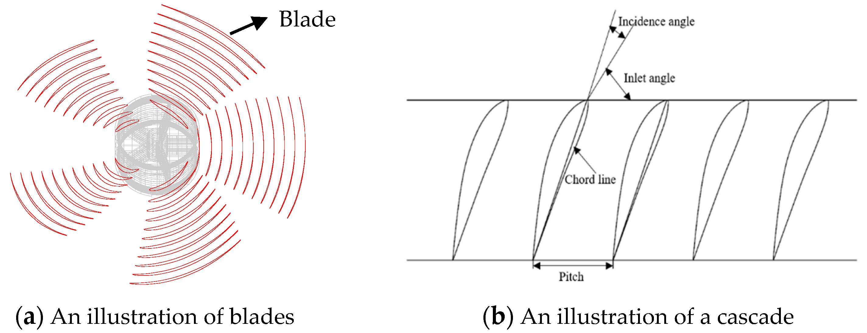
1. Introduction

Blade design is of great importance to the efficiency and properties of turbomachinery. Achieving the aerodynamic design of a blade is a very complex and arduous task due to complicated flow phenomena and the interactions among various parameters [1]. A small geometric change of one blade can lead to a deterioration of the aerodynamic performance of the whole machine [2]. In general, the cascade design method is one of the most popular design methods employed for turbomachinery [3,4]. In this method, the blade is stacked by the sections on the different radiuses and shown in Figure 1a. Additionally, the section is projected onto the plane to form the cascade, as shown in Figure 1b. Therefore, the blade performance is affected by the cascade design. With the rapid development of the computer technique, more and more parameterization methods and optimization algorithms have been proposed and used in the design process of a cascade. This means that the time required to design a new cascade is becoming shorter and the aerodynamic performance of the new cascade is becoming better.

A good parameterization method can not only use fewer design variables to describe an airfoil accurately, but also rapidly re-construct one airfoil in the optimization process [5,6]. The parameterization methods are usually divided into two categories: The constructive method and the deformative method. Each method has been continuously improved by many researchers [7]. The deformative parameterization method is the simpler of the two methods. In this method, a standard airfoil is deformed to generate one new airfoil, in order to satisfy a certain condition. The Hicks-Henne function [8], radial basis function [9], Bezier function [10], B-Spline function [11], and Non-Uniform Rational B-Splines (NURBS) function [12,13,14] are usually used as deformative functions to generate a new airfoil based on the original airfoil. In particular, NURBS [12] is the most popular function due to its ability of local control and its conics description over the curve. However, these deformative functions are used to generate one new airfoil based on the point coordinates of an airfoil. To relate the airfoil shape to the airfoil geometric feature parameters, the camber line superposing thickness distribution molding (CLSTDM) method [15] was proposed. In this method, several airfoil geometric parameters are used to parameterize the half-thickness distribution curve and the mean camber curve through two polynomials. Then, these two curves are coupled to form a whole airfoil. The feasibility of this method has been proved by several works [15,16,17]. In the CLSTDM method [15,16], the blade contours described by many coordinate points can be transformed into functions controlled by several parameterized variables. Moreover, it is convenient for designers to use this method to parameterize one blade based on their experience. Nowadays, it is widely used in the optimization of turbomachinery. However, the aerodynamic parameters are not considered in the parameterization and still act as the boundary condition of flow field computing.

To rapidly find the airfoil with the optimal aerodynamic property, many intelligent optimization technologies have been used in the process. Among all of the published optimization algorithms, the genetic algorithm (GA) [18,19,20,21] and the simulated annealing (SA) algorithm [10,11,22], as two traditional intelligent optimization algorithms, have been widely used in airfoil optimization. They aim to find the airfoil with the optimal performance precisely. However, much time is required to complete the search, which leads to a poor computational efficiency [23,24]. A new intelligent algorithm, known as particle swarm optimization (PSO) and proposed by Kenney and Eberhart [25], can be used to solve this problem. PSO is a population-based, self-adaptive searching optimization method. The principle of this method is based on animal social behaviors, such as birds’ migration. However, it is easy to become trapped into a local extreme value or converged to precocity by the standard PSO. Therefore, researchers began looking for improved methods to solve this problem. Shi [26] used a linearly decreasing inertia weight to balance the global and local searching character. However, the local searching capability of this method was weak. Simultaneously, it is hard to predict the maximum iteration number. Clerc [27] set a constriction factor determined by two learning factors to cancel the boundary limits of velocity, and to balance the global and local searching capability. Hu [28] adopted a stochastic inertia weight to replace the linearly decreasing inertia weight. This method could accelerate the convergence velocity and avoid being trapped into a local best solution. However, these methods still have the risk of local convergence.

Most approaches to parameterization of the cascade have been used with only the help of geometric feature parameters, and the aerodynamic parameters were not referred to. The efficiency of optimization was thus negatively affected. Therefore, in this paper, considering the cascade aerodynamic characters, one aerodynamic parameterization approach for a low Reynolds number cascade is proposed. To find the airfoil with the optimal performance during a certain range of incidence angles, a modified PSO-MVFSA algorithm is studied. Furthermore, two cases, such as the cascade with NACA4412 and the blade of FAN D500, are selected to verify the feasibility of the improved parameterization and optimization method.

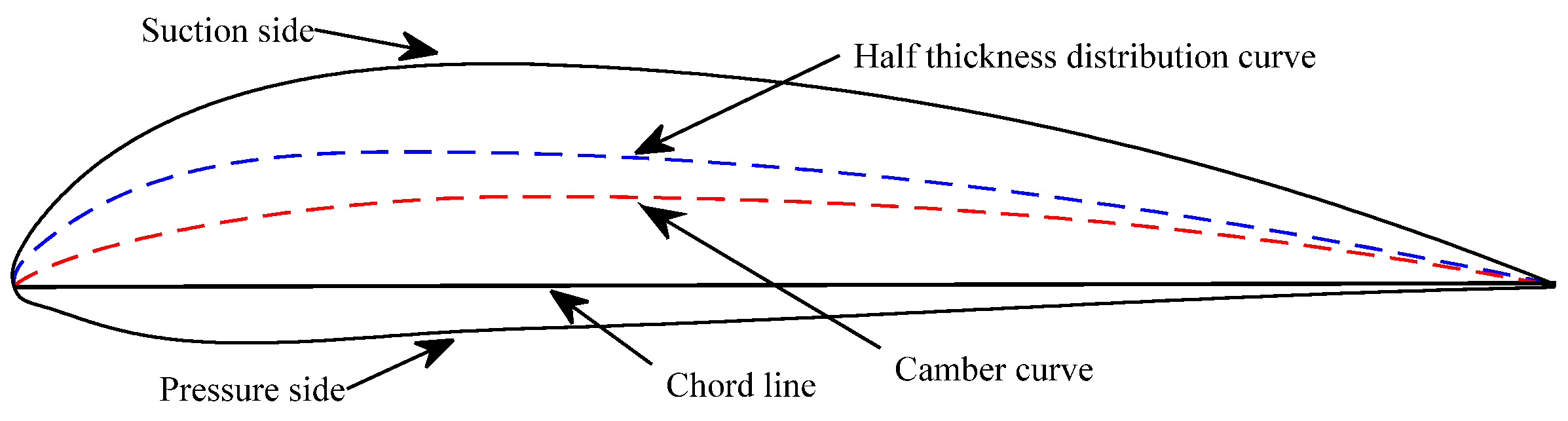
2. Aerodynamic Parameterization Method

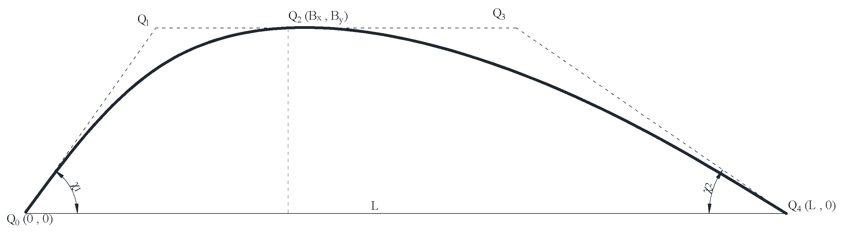
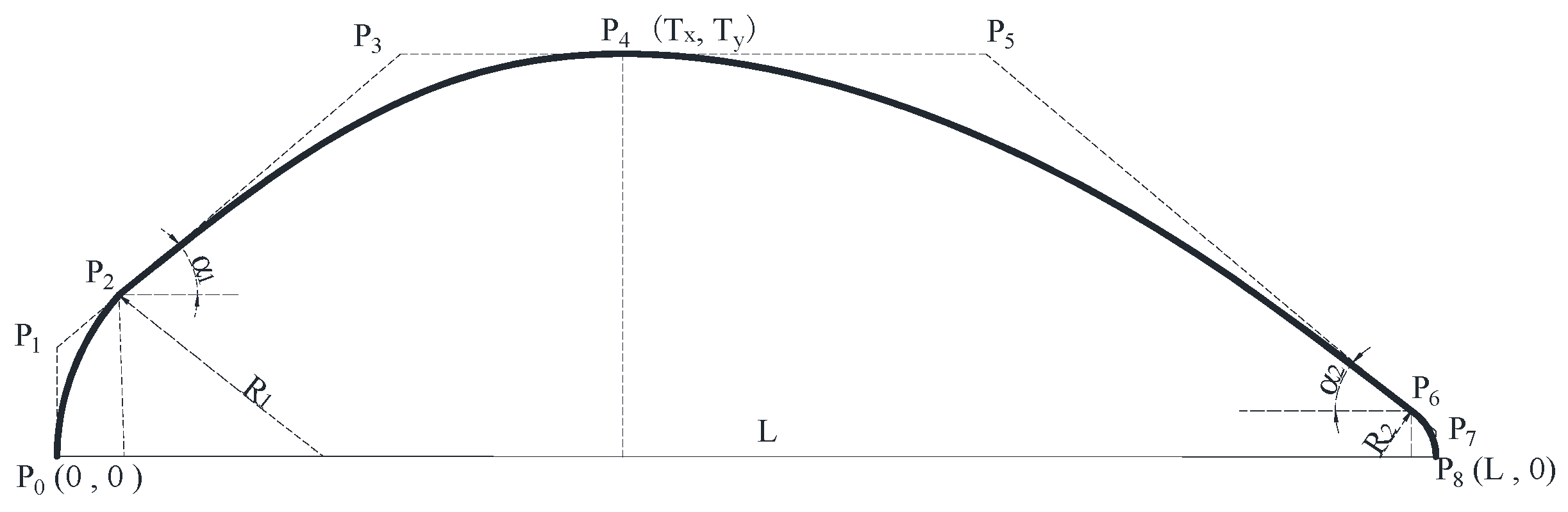
2.1. CLSTDM-NURBS Method

In this paper, for the CLSTDM method, the pressure side and suction side are obtained through the camber curve superposing the half-thickness distribution curve. This method is used to describe an airfoil and is shown in Figure 2. Due to its good ability to design a complex geometry, the two-order NURBS function defined by Equation (1) is used to describe the camber curve and the half-thickness distribution curve.

$$\{\begin{array}{l}C(u)={\displaystyle \sum _{i=0}^n}\frac{B_{2,i}\left(u\right){\omega }_i{Q}_i}{B_{2,i}{\omega }_i\left(u\right)}\\ B_{2,i}(u)=\frac{2!}{i!\left(2-i\right)!}{u}^i{\left(1-u\right)}^{2-i}\end{array},$$

(1)

where $u$ is the knot vector, $n$ is the order of NURBS ($n=2$), $i$ is the mark of the control points ($i=0,1,2$), $C(u)$ is the coordinate of the point of the fitting curve parameterized by the NURBS function, $B_{2,i}(u)$ is the Bernstain function, ${\omega }_i$ represents the weight coefficients (${\omega }_0=1,{\omega }_2=1$, ${\omega }_1=\omega$), and $Q_i$ is the control point. To solve the two-order NURBS function, the De Boor algorithm [29], which provides a fast and numerically stable way of finding a point on a B-spline curve with the given $u$ in the domain, is adopted and programed.

For camber parameterization, the camber curve is divided into two two-order NURBS curves (solid line), and these two NURBS curves are respectively controlled by several geometric control points ($Q_0,Q_1,Q_2$, $Q_3,Q_4$) shown in Figure 3. Five geometric feature parameters of an airfoil, such as the chord line $L=1.0$, the leading edge angle ${\chi }_1$, the trailing edge angle ${\chi }_2$, and the coordinate of the maximum camber point $\left(B_x,B_y\right)$, are adopted to derive the coordinates of the geometric control points of NURBS. To ensure the continuous property of two NURBS curves at the location of the maximum camber point $Q_2$, two lines $\overline{Q_1{Q}_2}$ and $\overline{Q_2{Q}_3}$ need to be collinear. Moreover, all of the geometric control points of NURBS are derived as follows in Equation (2).

$$\left[\begin{array}{l}{Q}_0\\ Q_1\\ Q_2\\ Q_3\\ Q_4\end{array}\right]=\left[\begin{array}{l}\left(0,0\right)\\ \left(B_y/\tan \left({\chi }_1\right),B_x\right)\\ \left(B_x,B_y\right)\\ \left(L-B_y/\tan \left({\chi }_2\right),B_y\right)\\ \left(L,0\right)\end{array}\right]$$

(2)

For parameterization of the half-thickness distribution curve, the curve is divided into three parts, including the leading edge half-thickness, the middle half-thickness, and the trailing edge half-thickness, as shown in Figure 4. The leading edge (LE) part is described by one two-order NURBS curve, the middle part by two two-order curves, and the trailing edge (TE) part by one two-order NURBS curve. Four NURBS curves are controlled by nine geometric control points ($P_0,P_1,P_2,P_3,P_4,P_5,P_6,P_7,P_8$), which are derived by seven geometric feature parameters of the airfoil, such as the leading edge radius $R_1$, the trailing edge radius $R_2$, the chord line $L=1.0$, the thickness gradient angles ${\alpha }_1,{\alpha }_2$, and the coordinate of the maximum half-thickness point $(T_x,T_y)$. As is the case for the camber curve, the half-thickness distribution curve also requires continuity. Therefore, at the three geometric control points $P_2,P_4,P_6$, it is necessary to maintain collinearity for the relative lines. Utilizing geometric principles, these control point coordinates are shown in Equation (3).

$$\left[\begin{array}{l}{P}_0\\ P_1\\ P_2\\ P_3\\ P_4\\ P_5\\ P_6\\ P_7\\ P_8\\ P_9\end{array}\right]=\left[\begin{array}{l}\left(0,0\right)\\ \left(0,R_1\ast \cos ({\alpha }_1)-R_1\ast \tan ({\alpha }_1)\ast (1-\sin ({\alpha }_1))\right)\tan ({\alpha }_1)\\ \left(R_1\ast (1-\sin ({\alpha }_1)),R_1\ast \cos ({\alpha }_1)\right)\\ \left(\left(T_y-R_1\ast \cos ({\alpha }_1)\right)/\tan ({\alpha }_1)+R_1\ast (1-\sin ({\alpha }_1)),T_y\right)\\ \left(T_x,T_y\right)\\ \left(-\left(T_y-R_2\ast \cos ({\alpha }_2)\right)/\tan ({\alpha }_2)+L-R_2\ast \left(1-\sin ({\alpha }_2)\right),T_y\right)\\ \left(L-R_2\ast \left(1-\sin ({\alpha }_2)\right),R_2\ast \cos ({\alpha }_2)\right)\\ \left(L,R_2\ast \cos ({\alpha }_2)-R_2\ast \tan ({\alpha }_2)\ast (1-\sin ({\alpha }_2))\right)\\ \left(L,0\right)\end{array}\right]$$

(3)

2.2. Improved Aerodynamic Parameterization

Unlike conventional parameterization approaches in which the airfoil is only parameterized with the geometric feature parameters [30,31,32], an improved aerodynamic parametrization approach combining the plane cascade design method and the CLSTDM-NURBS is proposed, in which the incidence angle, $i$, and nine geometric parameters are used as control variables.

For one specific cascade, it can be assumed for the airflow condition that the inlet flow angle ${\beta }_1$ is constant and along the tangential line. In this case, a change of the incidence angle can cause a change of the geometric inlet angle of the cascade, and the variation of the incidence angle $\Delta i$ is equal to that of the geometric inlet angle $\Delta {\beta }_{1A}$. From the definition of the geometric inlet angle, it is clear that the slope of the mean camber curve at the leading point is changed with the changing of the geometric inlet angle. This means that the variation of the incidence angle $\Delta i$ has an indirect influence on the modified value of the leading edge angle ${\chi }_1^{\prime }$. The relationship is shown in Equation (4).

$${\chi }_1^{\prime }={\chi }_1-\Delta i$$

(4)

Simultaneously, the deviation angle $\delta$ can also be affected by a change of the incidence angle. In order to determine the deviation angle, one semi-rational formula of the deviation angle was used, based on the plane cascade experiments by Howell [33,34], which was suitable for a low Reynolds number cascade and only applicable in the application conditions ($\tau =0.7~2.0$, $T_y=0.05~0.12$, and $B_x=0.4~0.5$). The definition formulas of the incidence angle $i$ and the deviation angle $\delta$ have been proposed in the cascade design process [3,35].

$$\tau =\frac{t}{L}$$

(5)

$$\delta ={\beta }_{2A}-{\beta }_2$$

(6)

In this paper, one special equation combining a semi-empirical formula [33,34] is shown in Equation (7), where $\phi$ is equal to $0.5$ for the rotor blade. Therefore, if the aerodynamic and geometric parameters $i$, $\tau$, ${\beta }_1$, ${\beta }_2$, and $B_x$ are given, the geometric outlet angle ${\beta }_{2A}$ can be calculated by Equation (7). Additionally, the revised trailing edge angle ${\chi }_2^{\prime }$ can be obtained by Equation (8). However, in Equation (7), it is found that the cascade solidity $\tau$ and the outlet flow angle ${\beta }_2$ cannot be determined.

$$\left({\beta }_{2A}-{\beta }_2\right)=\left[0.23{\left(2B_x\right)}^2-0.002{\beta }_2+0.18\right]\left({\beta }_{2A}-i-{\beta }_1\right){\left(\frac{1}{\tau }\right)}^{\phi }$$

(7)

$${\chi }_2^{\prime }={\chi }_2-\Delta {\beta }_{2A}$$

(8)

In order to obtain the abovementioned two parameters, the diffusion factor $D$ related to the cascade solidity $\tau$, the inlet flow angle ${\beta }_1$, and the outlet flow angle ${\beta }_2$, is introduced as a constraint. This coefficient can be used to control the aerodynamic load of the cascade. The definition of the diffusion factor is shown in Equation (9).

$$D=\left(1-\frac{\sin {\beta }_1}{\sin {\beta }_2}\right)+\frac{\sin {\beta }_1}{2\tau }\left(ctg{\beta }_1-ctg{\beta }_2\right)$$

(9)

Therefore, during the process of parameterization, the leading edge angle and trailing edge angle shown in Figure 3 are independent variables and no longer depend on the incidence angle. In this way, the control variables of cascade parameterization are determined, such as $B_x$, $B_y$, $T_x$, $T_y$, $R_1$, $R_2$, ${\alpha }_1$, ${\alpha }_2$, and $i$.

3. The Improved Airfoil Aerodynamic Optimization Method

3.1. Modified PSO-MVFSA

With the extensive use of standard particle swarm optimization (PSO), some drawbacks have been found, such as the local extreme minimum and the precocity. To solve these problems, many works have been published [26,27,28]. Some only adjusted the change of inertia weight to avoid being trapped into a local optimal solution. Moreover, some used two learning factors to balance the local searching and global searching. In this paper, the control variables of cascade parameterization are grouped as a particle. Additionally, the best particle position $X_{i,j}$ corresponding to the optimal cascade is obtained by the modified PSO, as shown in Equation (10) [27].

$$\{\begin{array}{ll}{V}_{i,j}^1& =\varphi ·\left[\omega V_{i,j}^0+c_1{\gamma }_1\left(P_{i,j}-X_{i,j}^0\right)+c_2{\gamma }_2\left(P_{g,j}-X_{i,j}^0\right)\right]\\ \varphi & =\frac{2}{\left|2-\left(c_1+c_2\right)-\sqrt{{\left(c_1+c_2\right)}^2-4\left(c_1+c_2\right)}\right|}\\ \omega & ={\mu }_{\min }+({\mu }_{\max }-{\mu }_{\min })\ast {\gamma }_4+\sigma ·{\gamma }_3\\ X_{i,j}^1& =X_{i,j}^0+V_{i,j}^1\end{array},$$

(10)

where $V$ is the particle velocity, subscript $i$, $j$ is the particle sequence, $\omega$ is the stochastic inertia weight [28], $\varphi$ is the constriction factor [27], $c_1$, $c_2$ represents two learning factors, ${\gamma }_1$, ${\gamma }_2$ represents the random number uniformly distributed in $\left(0,1\right)$, $P_{i,j}$ is the best position in its flight history, $P_{g,j}$ is the best position in the particle swarms, ${\mu }_{\max }$ is the maximum stochastic inertia weight, ${\mu }_{\min }$ is the minimum stochastic inertia weight, $\sigma$ is the variance of the stochastic inertia weight, and ${\gamma }_3$, ${\gamma }_4$ is the random number of the standard normal distribution.

However, it is very difficult to judge whether the results are the local optimal solutions or the global solutions when only using the modified PSO. Due to the probability of the simulated annealing (SA) algorithm jumping out of the local value, it can be used to solve the problem. Furthermore, considering that the low searching velocity of the standard SA algorithm can lead to a greater time consumption, modified very fast simulated annealing (MVFSA) [36] is adopted to search for the global optimal minimum. Since the Cauchy distribution depending on temperature was better than the Gaussian distribution, the coefficient of variable perturbation $y_{ij}$ based on the Cauchy distribution has been redefined by Equation (11). In order to improve the efficiency further, the random probability of the acceptance, $P_r$, has been redefined based on the Boltzmann–Gibbs distribution, as shown in Equation (12).

$$y_{ij}=T_{\max }\exp \left(-c{k}^{1/N_1}\right)·\mathrm{sgn}\left(u-0.5\right)\left[{\left(1+\frac{1}{T}\right)}^{\left|2u-1\right|}-1\right],$$

(11)

$$P_r={\left[1-\left(1-h\right)\left(E\left(M_{ij}^{\prime }\right)-E\left(M_{ij}\right)\right)/T\right]}^{1/\left(1-h\right)},$$

(12)

where $u$ is a random number ranging from $0$ to $1$, $T_{\max }$ is the initial simulated high temperature, $N_1$ is the syllogism coefficient, $k$ is the number of the marked annealing stage, $c$ is a given constant value, $M_{ij}^{\prime }$ is the disturbed variable, $M_{ij}$ is the undisturbed variable, and $h$ is a real number (set $h=0.5$). Furthermore, $E\left(M_{ij}\right)$ is adopted to evaluate the current energy of the particle.

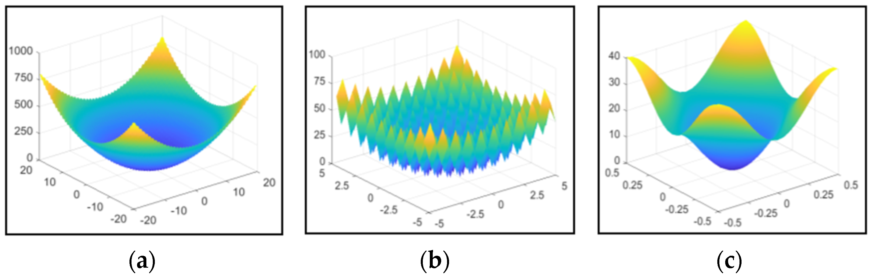
3.2. Verification of Modified PSO-MVFSA

Due to its local optimums and premature results, the Rastrigin function is usually used as a test function. The definition of the function is shown in Equation (13).

$$f(x)={\displaystyle \sum _{j=0}^D{x}_j^2}-10·\cos (2\pi x_j)+10x_j\in \left[-20,20\right]$$

(13)

In theory, when the independent variable $x_j$ is equal to $0$, the global minimum optimum of the function is $f(x_j)=0$. In Figure 5, three different solutions of the function are respectively shown. When the independent variable range is $\left[-20,20\right]$, the function looks smooth and monotonic, as shown in Figure 5a. With the increase of the resolution, many small peaks and valleys are observed in Figure 5b,c. This means that the function has many widespread local minima.

To prove the feasibility and accuracy of the modified PSO-MVFSA, two other PSO-based optimization algorithms, as two comparison algorithms, are adopted to search for the optimal minimum of the Rastrigin function. As the function is two-dimensional, each particle consists of two variables for three kinds of PSO algorithms. The initial particle number, the total iteration number of PSO, and the total iteration number of MVFSA are set to 30, 80, and 40, respectively. Some other coefficients are listed in

Table 1. Coefficients of three algorithms based on particle swarm optimization (PSO).

Maximum Stochastic Inertia Weight, ${\mathit{\mu }}_{\mathbf{max}}$	Minimum Stochastic Inertia Weight, ${\mathit{\mu }}_{\mathbf{min}}$	Variance Stochastic Inertia Weight, $\mathit{\sigma }$	Learning Factor, ${\mathit{c}}_{\mathbf{1}}$	Learning Factor, ${\mathit{c}}_{\mathbf{2}}$
0.8	0.4	0.2	2.25	1.85
The Initial Simulated High Temperature, ${\mathit{T}}_{\mathbf{max}}$	The Final Cooling Simulated Temperature, ${\mathit{T}}_{\mathbf{min}}$	The Syllogism Coefficient, ${\mathit{N}}_{\mathbf{1}}$	The Positive Value, $\mathit{\alpha }$	Markov Chain Length, $\mathit{J}$
30	0.0001	9	0.8	15

, such as the positive value $\alpha$, the Markov chain length $J$, and so on. By means of these searching optimization methods, the optimal results are obtained and shown in

Table 2. Results of three algorithms based on PSO.

Algorithms	Computing Time $\mathit{T}$ (Seconds)	Optimal Particle ${\mathit{x}}_{\mathit{o}\mathit{p}\mathit{t}}$	Optimal Function Value $\mathit{f}\left({\mathit{x}}_{\mathit{o}\mathit{p}\mathit{t}}\right)$
Standard PSO [22]	1.08942	(0.001225, −0.000958)	0.000481
PG-PSO [21]	1.14177	(−0.001495, 0.0000077)	0.000443
PSO -MVFSA	0.898254	(0.000177, −0.000476)	0.000051

. It can be seen that the optimal function value obtained by PG-PSO is smaller than that of the standard PSO. However, the computing time is longer than that of the standard PSO. For the modified PSO-MVFSA, not only its time consumption, but also its ability for minimum searching, are optimal in comparison with the other two algorithms.

3.3. The Improved Airfoil Aerodynamic Optimization

3.3.1. Fitness Function

For improved cascade aerodynamic optimization, nine control variables are used to parameterize the cascade and grouped as a particle. In all flights, the selection of the particle with the best position through the optimum target is very important. The lift-drag ratio of the airfoil is related to its capability regarding the power output and aerodynamic loss [16]. Therefore, the optimization proposition is set up as shown in Equation (14).

$$\{\begin{array}{l}f\left(S_1,S_2\cdots S_{10}\right)={\displaystyle \sum _{i=1}^n{\left(C_L/C_D\right)}_i}/n\\ s.t.\\ {\chi }_1>\arctan \left(B_y/B_x\right)-{\chi }_2>\arctan \left(B_y/\left(1-B_x\right)\right)\\ {\alpha }_1>\arctan \left(T_y/T_x\right)-{\alpha }_2>\arctan \left(T_y/\left(1-T_x\right)\right)\\ 0.4\le D\le 0.6\end{array},$$

(14)

where $S_i$ is the control variable, $C_L/C_D$ is the lift-drag ratio, $\left(B_x,B_y\right)$ is the coordinate of the maximum camber point, $\left(T_x,T_y\right)$ is the coordinate of the maximum half-thickness point, ${\alpha }_1$, ${\alpha }_2$ represent the LE and TE thickness gradient angles, ${\chi }_1$, ${\chi }_2$ represent the LE and TE angles, and $n$ is the number of incidence angles. In this paper, the average lift-drag ratio of the airfoil is evaluated under all airflow incidence angles. Additionally, the fitness function can be obtained as shown in Equation (15).

$$\begin{array}{l}-F=c_1\frac{f\left(S_1,S_2\cdots S_{10}\right)-{\displaystyle \sum {\left(C_L/C_D\right)}_{ref}}}{{\displaystyle \sum {\left(C_L/C_D\right)}_{ref}}}+c_2\frac{{\alpha }_1-\arctan \left(B_y/B_x\right)}{\arctan \left(B_y/B_x\right)}-c_3\frac{{\alpha }_2+\arctan \left(B_y/\left(1-B_x\right)\right)}{\arctan \left(B_y/\left(1-B_x\right)\right)}\\ +c_4\frac{X_1-\arctan \left(T_y/T_x\right)}{\arctan \left(T_y/T_x\right)}+c_5\frac{-X_2-\arctan \left(T_y/\left(1-T_x\right)\right)}{\arctan \left(T_y/\left(1-T_x\right)\right)}+c_6\left(D_i-D\right)\end{array}$$

(15)

where $c_i$ is the weighting factor and subscript $ref$ presents the original airfoil.

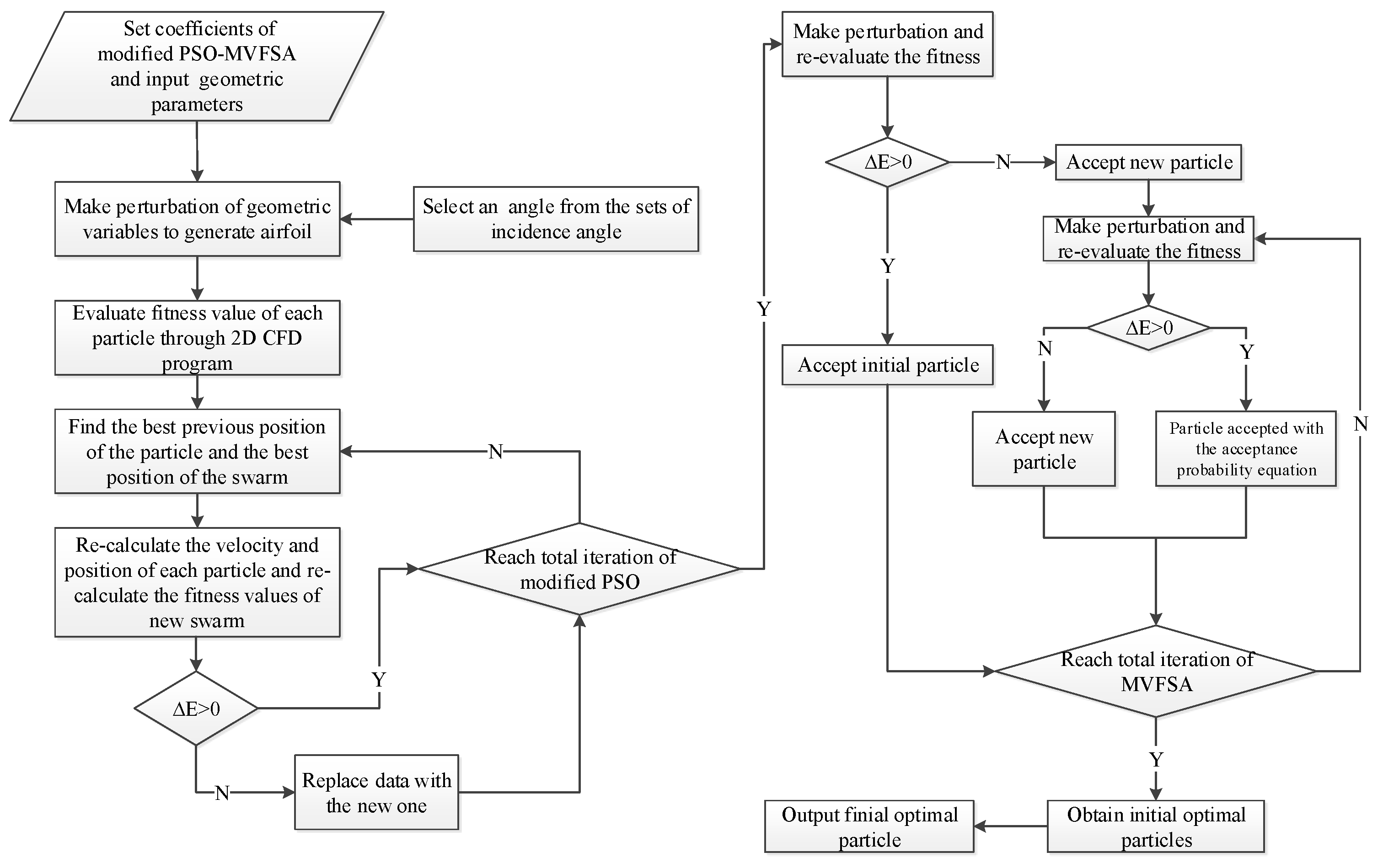
3.3.2. Aerodynamic Optimization Process

During the evaluation of airfoil aerodynamic performance two-dimensional computational fluid dynamics (2D CFD) code which utilized the standard $k-\omega$ turbulence model [37,38] to solve the Reynolds Average Navier-Stokes (RANS ) equations was used, and it was only used to simulate the low Reynolds number airfoils [23,39]. Due to the fact that the lift-drag ratio of one airfoil could be obtained quickly by this code, this 2D CFD code was integrated into MATLAB as a fast solver to evaluate the fitness value of each particle. The whole aerodynamic optimization flowchart is shown in Figure 6. Moreover, the detailed process is introduced in the following steps:

(a)

Inputting coordinate points of one airfoil, and setting coefficients of the modified PSO-MVFSA;

(b)

Selecting one angle from the sets of incidence angles and nine geometric variables as an initial particle;

(c)

Conducting perturbation of nine geometric variables of the initial particle to generate the initial particle swarm with one incidence angle, based on the super Latin square method; constructing airfoil swarm by the improved parameterization method; and evaluating the airfoil fitness value by Equation (15);

(d)

Finding the best previous position of the particle and the best position of the swarm, re-calculating the velocity and the position of each particle by adopting Equation (10), and re-calculating the fitness values of the new swarms;

(e)

If $\Delta E>0$ ($\Delta E=E\left(M_{ij}^{\prime }\right)-E\left(M_{ij}\right)$ is the error function), the data related to the particle are unchanged; if not, replace the data and particles with new data and particles;

(f)

Repeating steps (d) and (e) until the total iteration of the modified PSO is reached;

(g)

Obtaining the swarm particles ${\left(S\right)}_i$ that satisfy $\left[F_{opt}-F\left({\left(S\right)}_i\right)\right]/F_{opt}<10\%$;

(h)

Putting the swarm particles ${\left(S\right)}_i$ into the optimization process of MVFSA, conducting perturbation, and re-evaluating the fitness by Equation (10);

(i)

If $\Delta E>0$, the corresponding particle is preserved; if not, the corresponding particle as a basic particle is re-disturbed and re-evaluated;

(j)

If $\Delta E>0$, the re-disturbed particle is retained; if not, the particle is accepted with the acceptance probability equation;

(k)

Repeating steps (g) (h) (i) until the total iteration of MVFSA is reached;

(l)

Outputting the particle with the largest function $F$ from the preserved particle swarm at different incidence angles respectively;

(m)

Selecting the best of the optimal particles by MVFSA as the final optimal particle.

4. Applications in Cascade Optimization

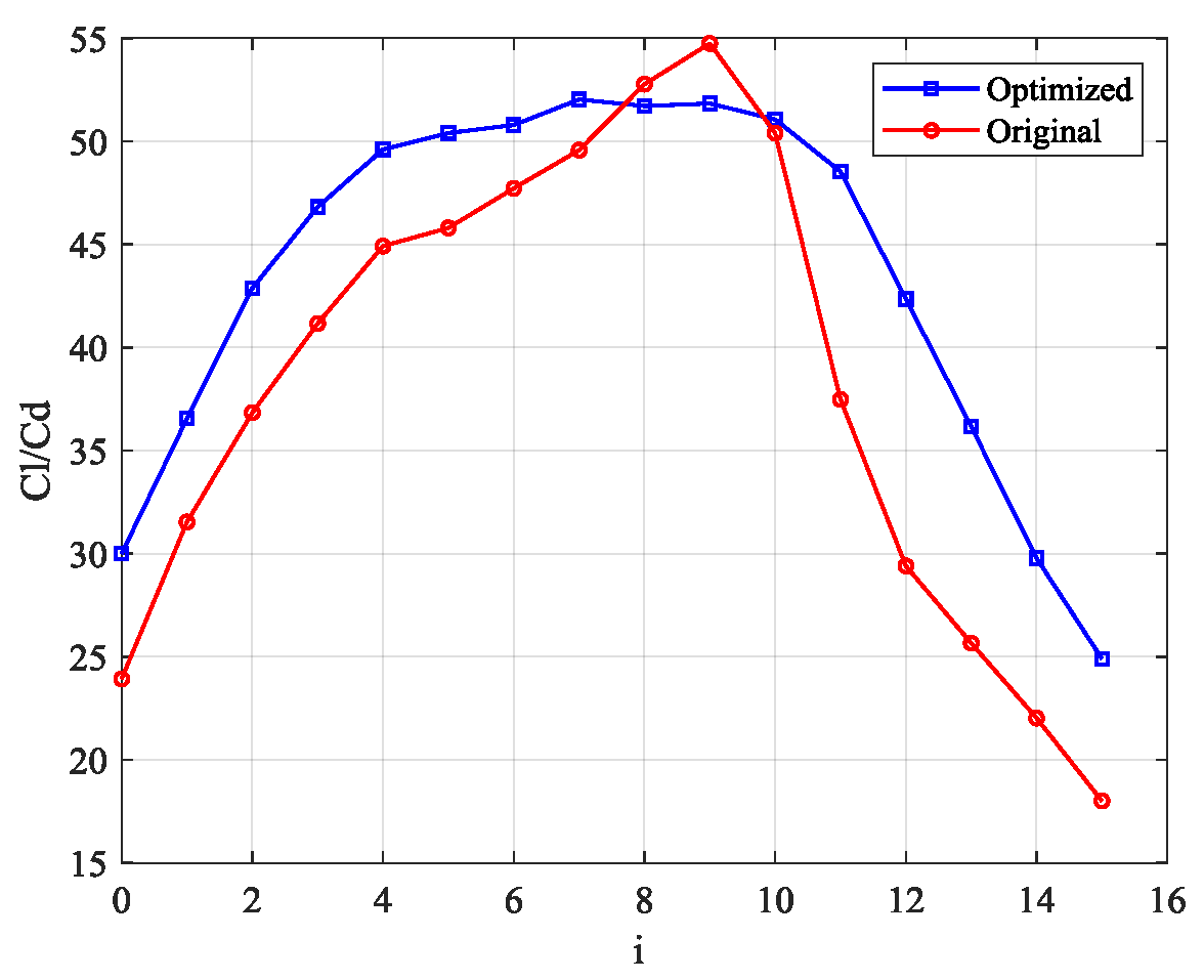
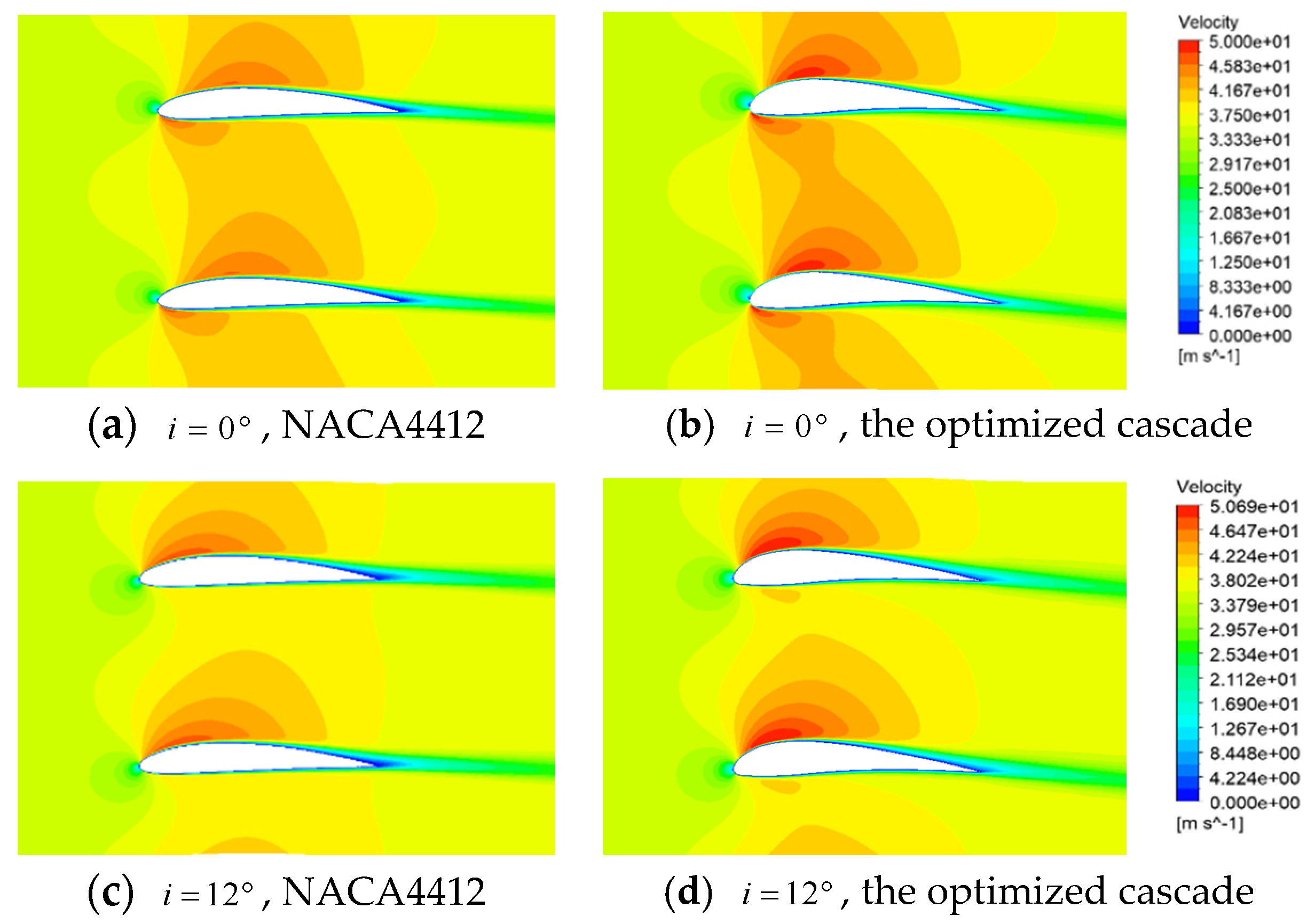
4.1. Optimization of a Cascade with an NACA4412 Profile

NACA4412 is adopted as the original basic profile of the cascade and evolved into an advanced airfoil by this improved method. The initial particle number, the total iteration number of the modified PSO, and the total iteration number of MVFSA are set to 30, 100, and 50, respectively. Each cascade is described by the improved aerodynamic parameterization method. The average lift-drag ratio of the airfoil of the cascade is calculated by the flow solver. Moreover, the constant airflow boundary condition is set so that the Reynolds number is as high as $1\times {10}^5$, the Mach number is $0.1$, and the solidity of the cascade is $1.5$. Moreover, some other coefficients of the modified PSO-MVFSA are shown in

Table 3. Coefficients of modified PSO-modified very fast simulated annealing (MVFSA).

Maximum Stochastic Inertia Weight, ${\mathit{\mu }}_{\mathbf{max}}$	Minimum Stochastic Inertia Weight, ${\mathit{\mu }}_{\mathbf{min}}$	Variance Stochastic Inertia Weight, $\mathit{\sigma }$	Learning Factor, ${\mathit{c}}_{\mathbf{1}}$	Learning Factor, ${\mathit{c}}_{\mathbf{2}}$
0.8	0.4	0.2	2.25	1.85
The Initial Simulated High Temperature, ${\mathit{T}}_{\mathbf{max}}$	The Final Simulated Cooling Temperature, ${\mathit{T}}_{\mathbf{min}}$	The Syllogism Coefficient, ${\mathit{N}}_{\mathbf{1}}$	The Positive Value, $\mathit{\alpha }$	Markov Chain Length, $\mathit{J}$
40	0.0001	9	0.8	20

.

In actual airflow conditions, the incidence angle of the cascade is not constant and limited to a certain range. Therefore, the aim of multi-point optimization is not to obtain the best aerodynamic performance under one constant incidence angle, but to reach the best whole aerodynamic performance in the whole working range, referred to in Equation (12). In this paper, the incidence angle is uniformly distributed from 0° to 15° by a step of 1.0°. The aerodynamic performance of each cascade parameterized by one incidence angle and eight geometric variables is calculated by the CFD simulation. Based on Equation (13), the fitness value corresponded to each cascade is figured out. Then, the global minimum value is found by the user of the improved PSO-MVFSA method. NACA4412 airfoil and the optimal airfoil are shown in Figure 7, in which the blue curve is the optimal airfoil and the red curve denotes the original airfoil. From this figure, it can be observed that the suction side and pressure side of the optimized airfoil are changed in terms of geometry in comparison with that of NACA4412.

To evaluate the aerodynamic performance of the cascade, the pressure coefficient $C_p$ is adopted, which is defined by Equation (16).

$$C_p=-\left(\frac{p-p_{\infty }}{\frac{1}{2}\rho u_{\infty }^2}\right)=\frac{p_{\infty }-p}{p_0-p_{\infty }},$$

(16)

where $p$, $p_0$, $p_{\infty }$ are the current pressure, the stagnation pressure, and the inlet airflow pressure, respectively; $\rho$ is the density; and $u_{\infty }$ is the inlet airflow velocity.

The increasing curvature of the suction side close to LE can lead to the intensifying of the velocity increasing and the pressure decreasing. Then, the pressure coefficient of the suction side of the optimized $C_p$ near LE is larger than that of the original cascade. However, it is due to the geometric change of the pressure side close to LE that the decreasing of the velocity and the increasing of the pressure are alleviated. These phenomena can be observed in Figure 8. In the figure, the detailed pressure distributions on the suction and pressure side are shown, which respectively correspond to four incidence angle conditions of $i=0°$, $i=3°$, $i=6°$, and $i=12°$. It is also clear that the optimized airfoil surface pressure distribution presented by the blue curve is better than that of the original airfoil described by the red curve under each condition. Therefore, the pressure differences between the pressure side and suction side of the optimized airfoil are larger than those of the original airfoil. The cascade performances under the incidence angles ranging from 0° to 15° are shown in Figure 9. The average lift-drag ratio of the optimized cascade is increased by 13.38% in comparison with that of the cascade with NACA4412.

For further analysis, CFD simulation software CFX was used to calculate the cascade performance. The velocity contours of the original and optimized cascades at incidence angles of $i=0°$ and $i=12°$ are shown in Figure 10. It is clear that the velocity difference between the suction side and pressure side of the optimized cascade is bigger than that of NACA4412. Therefore, the diffusion factor $D$ of the optimized cascade can be increased. It can also be observed that the airflow separation point on the suction side of the optimized cascade moves backward along the airfoil in comparison with that of NACA4412 and the area of the wake becomes smaller than that of NACA4412. Therefore, it can be considered that the aerodynamic load of the cascade is increased and the aerodynamic loss is controlled with the help of the improved aerodynamic optimization algorithm.

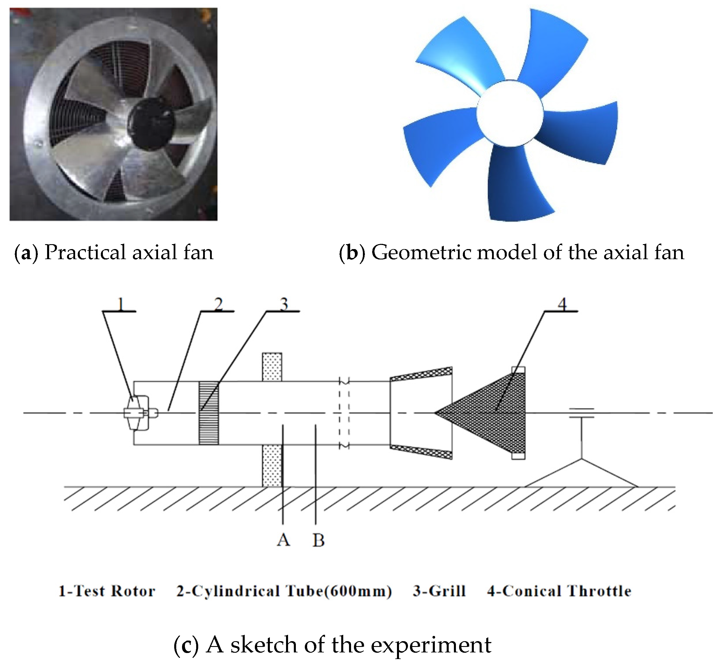
4.2. Blade D500 Optimization

Blade D500 is used in an axial-flow fan for an evaporator system. It is a kind of low Reynolds number 3D blade. In this work, in order to verify the feasibility of the improved method applied to the practical blade design, the cascade at the 50% radius of Blades D500 was selected and optimized. Two performance parameters, including the pressure coefficient $C_p$ defined by Equation (16) and the efficiency $\eta$ defined by Equation (17), were used to evaluate the aerodynamic performance of Blade D500. In order to obtain the aerodynamic performance parameters, CFX was used to calculate the airflow field of Blade D500.

$$\eta =\frac{Q_v·P}{N},$$

(17)

where $Q_v$ is the volume flow rate, $P$ is the static pressure increase, and $N$ the aerodynamic power.

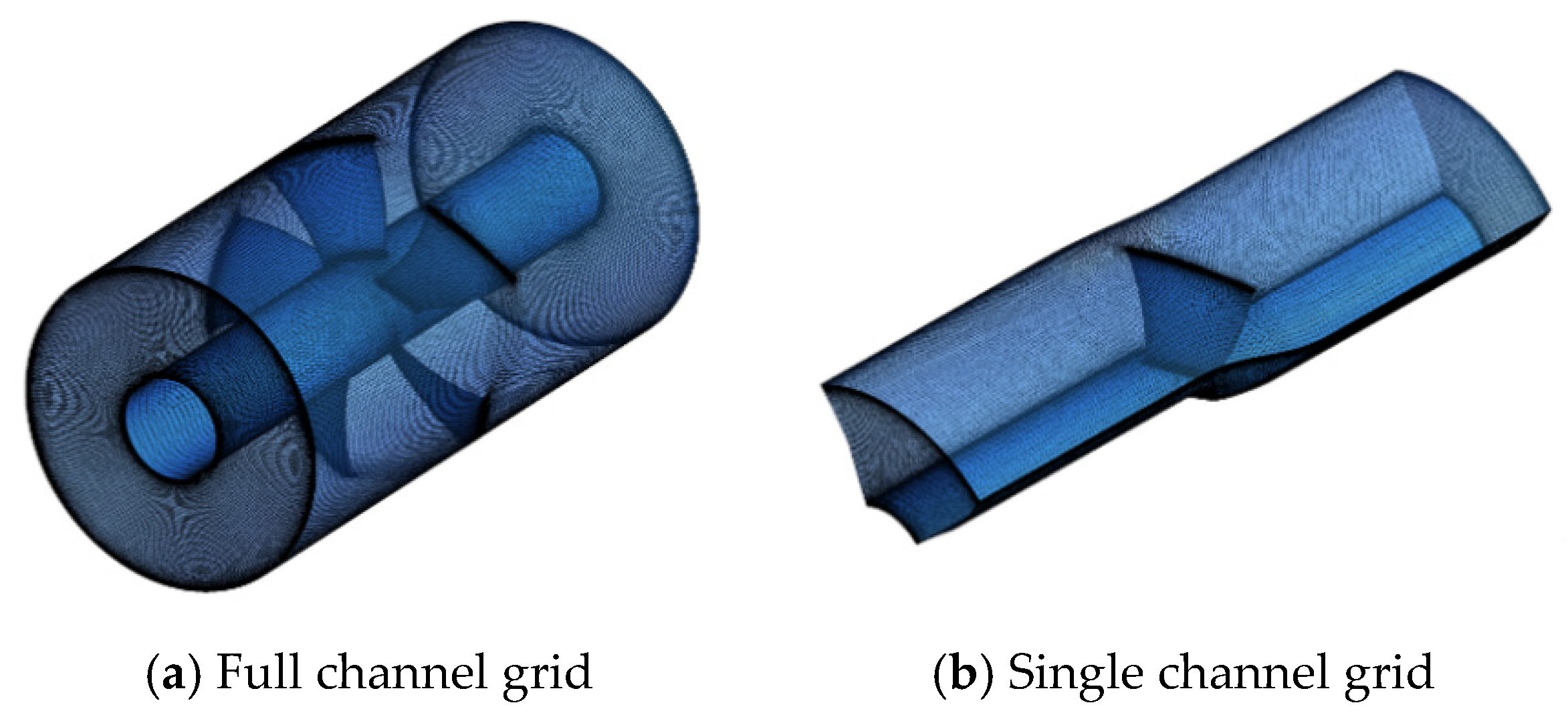
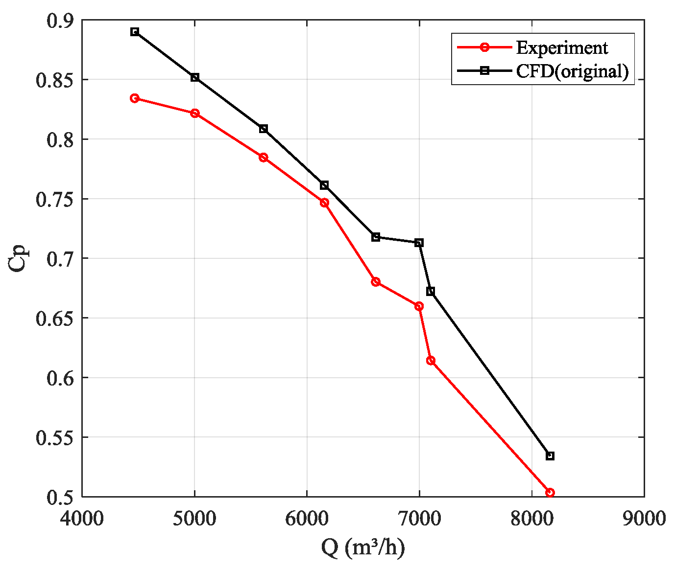
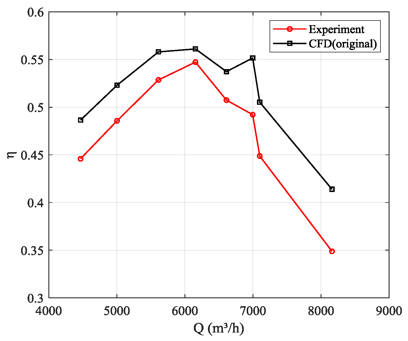
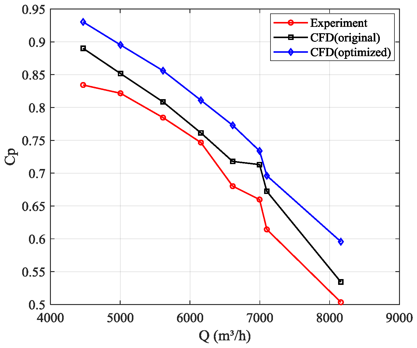
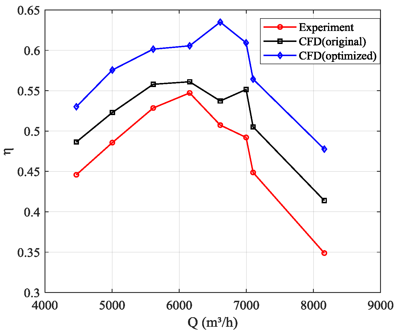
4.2.1. Validation of the CFD Simulation Based on Experiments

The experiments of the axial fan with Blade D500 shown in Figure 11 were conducted in the Key Lab for Power Machinery and Engineering of SJTU. In order to match the practical situation, the rotor was mounted on the guard grill, which was connected with a short bell month at the inlet of the tube. The diameter of the tube was increased to 600 mm to avoid destroying the flow field at the rotor outlet and simulate the real situation in the evaporator system as much as possible. The pressure probes were mounted at points A and B, by which the flow rate and the pressure increase could be calculated. Under eight volume flow rates, the pressure increases were calculated.

Under the same conditions as those used in the experiments, CFX was adopted to simulate the aerodynamic performance of the axial fan. The grids consisted of the structured hexahedral meshes shown in Figure 12 that were generated by TurboGrid. The total number of nodes was 1,260,626 for the full channel after studying the grid independence, and the minimum value of the mesh quality was 0.3. Due to the excellent ability to simulate the flow with a fiercely adverse pressure gradient of the standard $k-\omega$ model, it was selected as the turbulent model to simulate the flow field. The mass flow and static pressure were set at the inlet and outlet, respectively.

After a series of experiments and CFD simulations of the axial fan with Blade D500, the pressure coefficients were obtained and are shown in Figure 13. Based on Figure 13, it could be found that the pressure coefficients $C_{sp}$ calculated by CFD are slightly higher than those calculated by experiments. However, the trends of the two curves are very similar. In Figure 14, the efficiency is compared for values obtained by calculations and experiments. It can be observed that the relative error between the two series of average efficiencies is under 8.35%. Considering the abovementioned results, the CFD simulation can be used to feasibly estimate the aerodynamic performance of an axial fan.

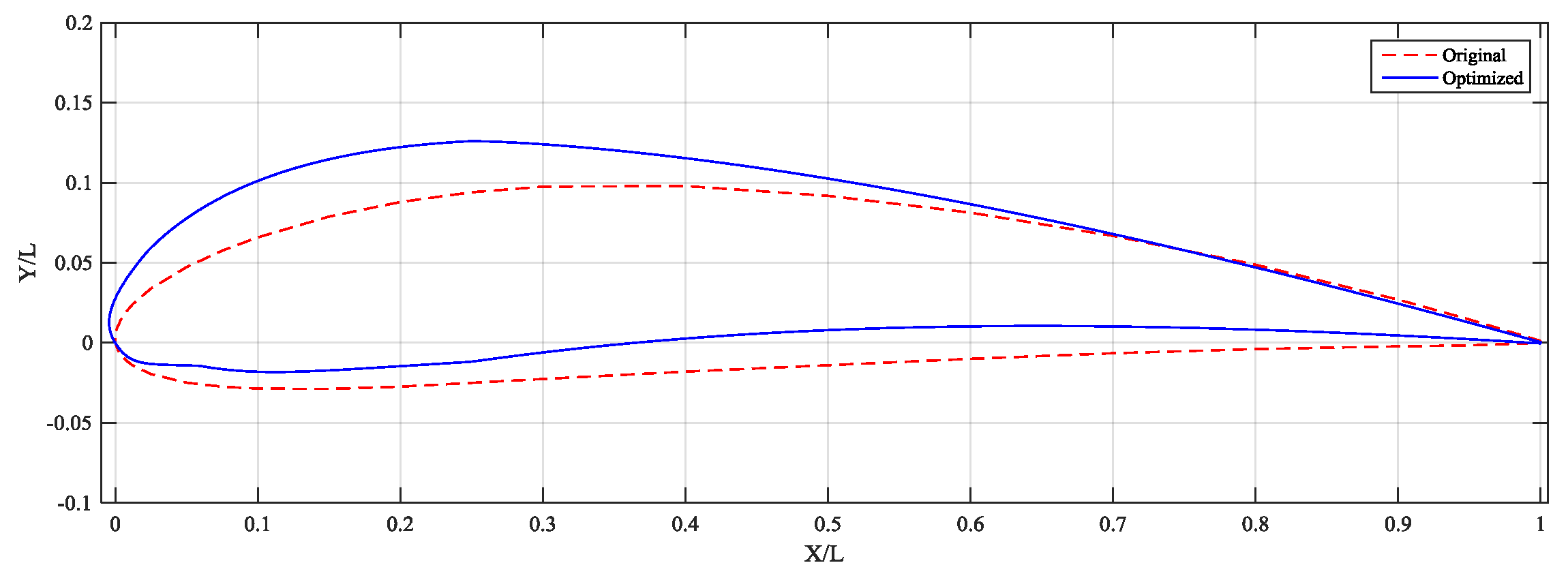
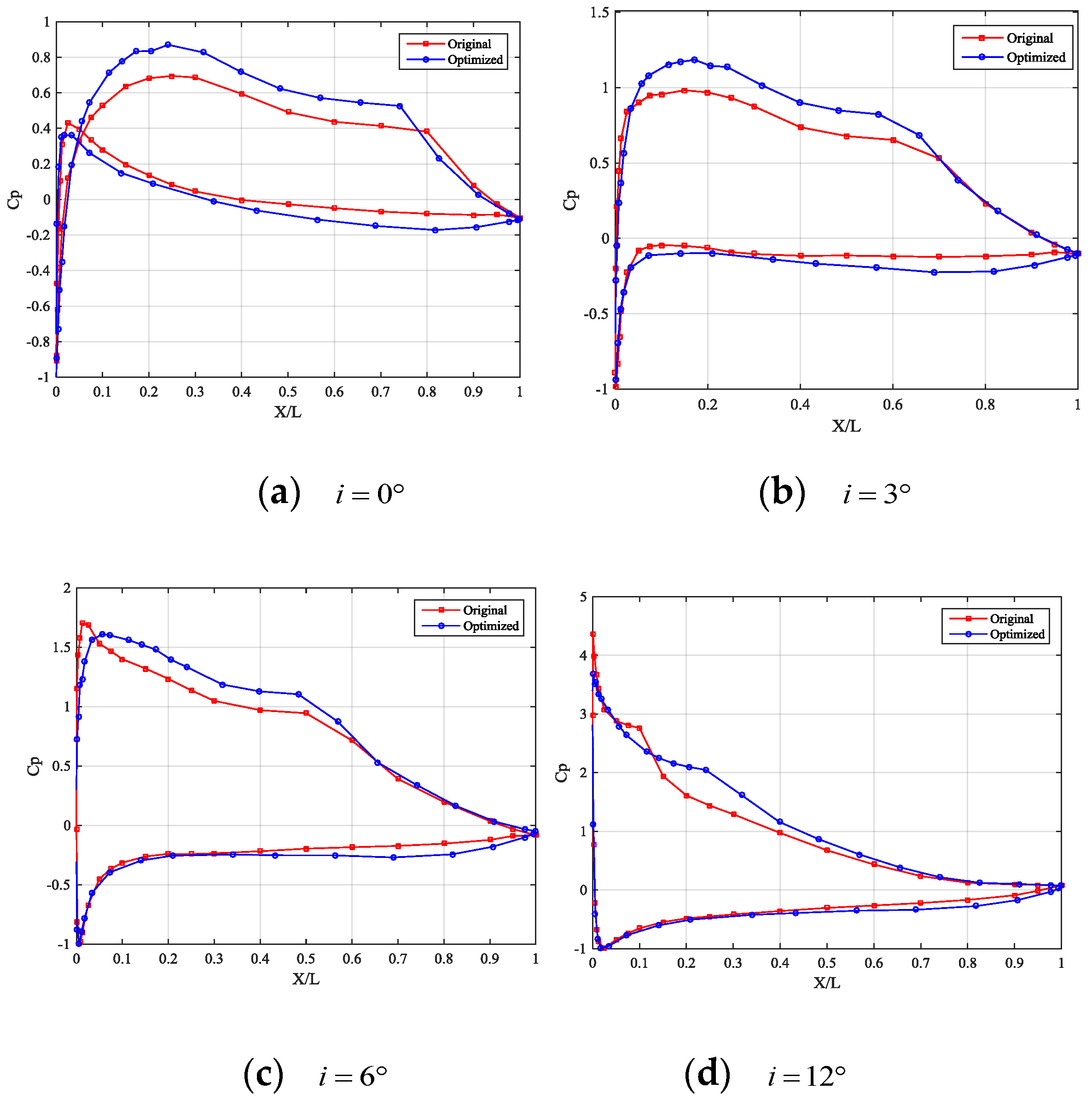
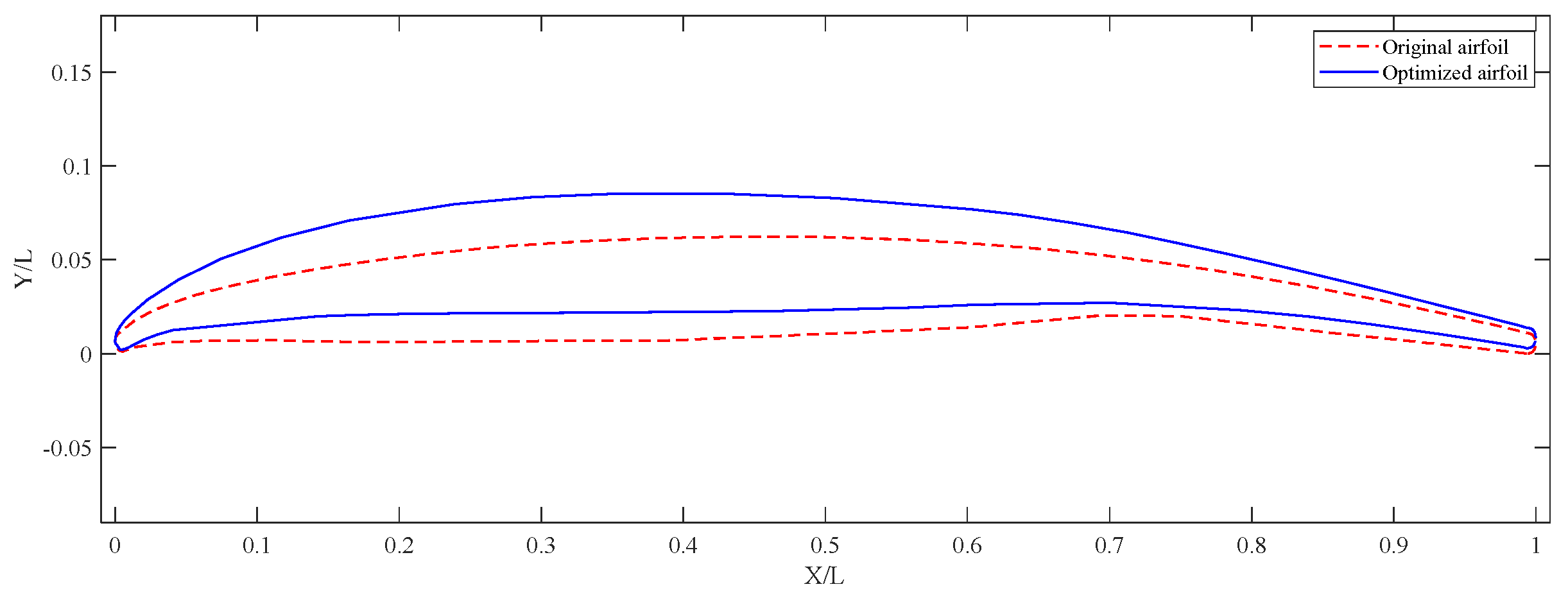
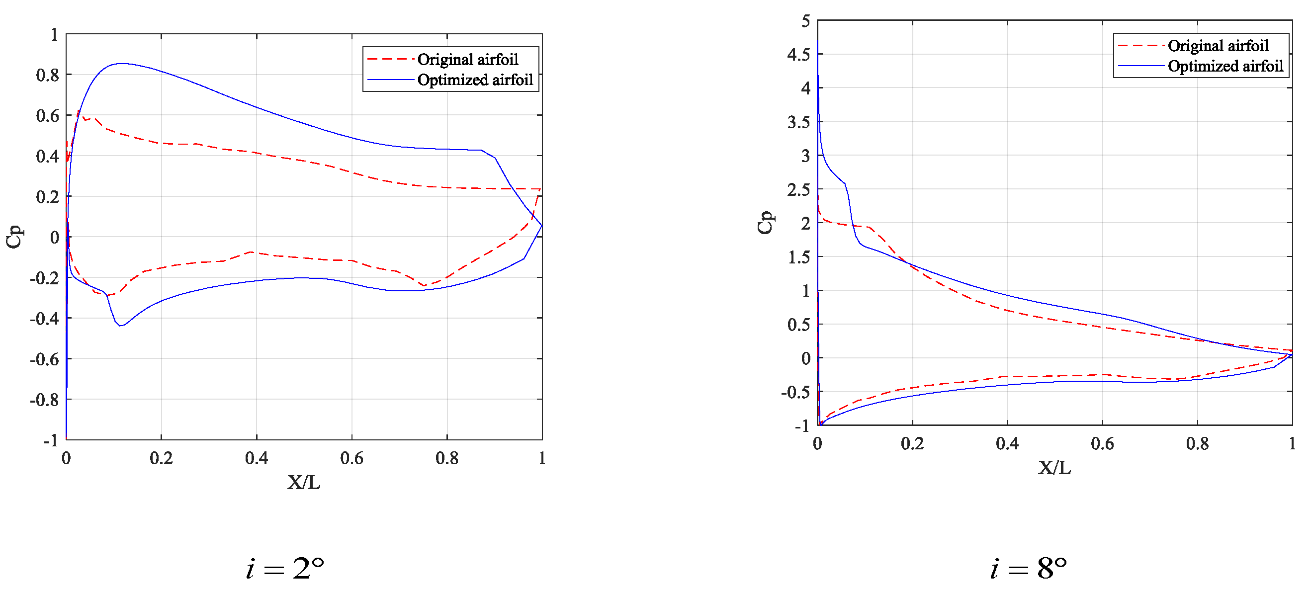
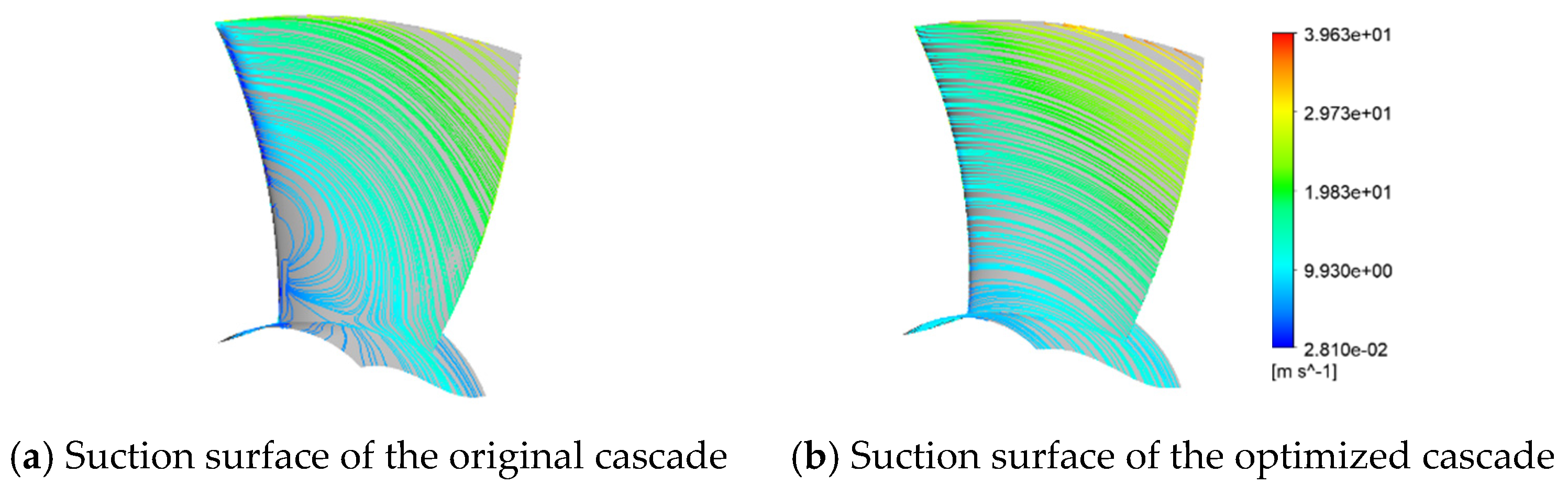
4.2.2. Optimization of Blade D500

For aerodynamic optimization of the cascade at the 50% radius of Blade D500, the airflow condition was set as $\mathrm{Re}=1\times {10}^5$, $Ma=0.1$, $i=2°\sim 10°$, $D=0.4\sim 0.6$. After a series of optimization iterations, the airfoil of the optimal cascade was obtained and is shown in Figure 15, as well as the airfoil of the original cascade. It can be observed that the airfoil of the optimized cascade is different from that of the original cascade. These geometric changes of the optimal cascade can lead to an increase of the curvature of the suction side, while the pressure side is changed a little. Additionally, aerodynamic performance comparisons are shown in Figure 16. It could be found that the pressure differences of the optimized cascade are larger than those of the original airfoil along the chord line within the range of the incidence angle. After a series of simulation calculations, it could be found that the average lift-drag ratio of the optimized cascade is increased by 15.21% in comparison with that of the original cascade. Therefore, it can be considered that the aerodynamic performance of the optimized cascade is better than that of the original one.

To evaluate the feasibility of the improved aerodynamic optimization method, the optimized 3D Blade D500 and the original 3D Blade D500 were simulated by CFD under the same airflow condition. Moreover, the simulation results of two blades were compared. The streamlines of the suction surfaces of the two blades are shown in Figure 17. From the figure, it is clear that the streamline between the middle section and the hub of the original blade is not very good, and a large turbulence loss must have occurred in this region. In contrast, the streamline in the same region of the optimized blade becomes very smooth. The pressure coefficients $C_{sp}$ of the two fans are shown in Figure 18. In this figure, it can be seen that the pressure coefficient of the optimized fan is better than that of the original fan, and the average pressure coefficient is increased by 6.12%. Meanwhile, from Figure 19, it can be observed that the efficiency of the optimized fan is higher than that of the original one, and averagely increased by 11.15%. Therefore, from the above analysis, it can be considered that the aerodynamic performance of optimized Blade D500 is improved and the improved aerodynamic optimization method is feasible.

5. Conclusions

In this paper, an improved optimization method especially applied to a cascade with a low Reynolds number is proposed. In this method, the incidence angle and eight geometric parameters are used as the control variables altogether. Meanwhile, the modified PSO-MVFSA algorithm is adopted to optimize the objective cascades, and two cascade cases, such as NACA4412 and Blade D500, are selected to testify the method. Some valuable results are as follows:

(a)

Since the aerodynamic parameter, such as the incidence angle, is considered as one of the control variables, the relationship between the geometry of the airfoil and the aerodynamic performance of the cascade is learnt. Therefore, during the whole optimization process, an improvement of the aerodynamic performance can give rise to a direct modification of the geometry so that the optimization becomes more targeted and more efficient;

(b)

In this study, particular effort was devoted to designing a fitness function which is suitable for optimizing a cascade with a low Reynolds number. Furthermore, the combination of PSO and MVFSA succeeded in increasing the optimization efficiency and avoided the local optimal to reach a global solution, which was verified by the Rastrigin function and two cascade cases;

(c)

Based on the analysis of the results from the two cascade cases, such as NACA4412 and Blade D500, it was demonstrated that the average lift-drag coefficient of the optimized cascade was improved, whilst the drag coefficient was kept at a low level. Therefore, it can be considered that the modified PSO-MVFSA can be adopted as an efficient and robust optimizer to solve the problems of multi-variable optimization confronted in cascade design.

References

- Li, Z.; Zheng, X. Review of design optimization methods for turbomachinery aerodynamics. Prog. Aerosp. Sci. 2017, 93, 1–23. [Google Scholar] [CrossRef]
- Garzon, V.E.; Darmofal, D.L. Impact of geometric variability on axial compressor performance. J. Turbomach. 2003, 125, 692–703. [Google Scholar] [CrossRef] [Green Version]
- Eck, B. Ventilatoren; Springer: Berlin/Heidelberg, Germany, 1991. [Google Scholar]
- Batyaev, E.A.; Kurzin, V.B. Method of optimization of blade shapes in aerodynamic design of the fan cascade. J. Appl. Mech. Tech. Phys. 2002, 43, 701–705. [Google Scholar] [CrossRef]
- Wu, H.-Y.; Yang, S.; Liu, F.; Tsai, H.-M. Comparisons of three geometric representations of airfoils for aerodynamic optimization. In Proceedings of the 16th AIAA Computational Fluid Dynamics Conference, Orlando, FL, USA, 23–26 June 2003. [Google Scholar]
- Samareh, J.A. Survey of shape parameterization techniques for high-fidelity multidisciplinary shape optimization. AIAA J. 2001, 39, 877–884. [Google Scholar] [CrossRef]
- Mahmood, S.M.H.; Turner, G.M.; Siddappaji, K. Flow characteristics of an optimized axial compressor rotor using smooth design parameters. In Proceedings of the ASME Turbo Expo 2016, GT2016, Seoul, Korea, 13–17 June 2016. [Google Scholar] [CrossRef]
- Hicks, R.M.; Henne, P.A. Wing design by numerical optimization. J. Aircr. 1978, 15, 407–412. [Google Scholar] [CrossRef]
- Buhmann, M.D. Radial basis functions. New Algorithms Macromol. Simul. 2004, 37, 31–65. [Google Scholar] [CrossRef]
- Liu, J.-L. A novel Taguchi-simulated annealing method and its application to airfoil design optimization. In Proceedings of the 17th AIAA Computational Fluid Dynamics Conference, Toronto, ON, Canada, 6–9 June 2005. [Google Scholar] [CrossRef]
- Chao, S.-M.; Whang, A.J.-W.; Chou, C.-H.; Su, W.-S.; Hsieh, T.-H. Optimization of a total internal reflection lens by using a hybrid Taguchi-simulated annealing algorithm. Opt. Rev. 2014, 21, 153–161. [Google Scholar] [CrossRef]
- Ghaly, W.S.; Mengistu, T.T. Optimal geometric representation of turbomachinery cascades using NURBS. Inverse Probl. Eng. 2003, 11, 359–373. [Google Scholar] [CrossRef]
- Sonoda, T.; Yamaguchi, Y.; Arima, T.; Olhofer, M.; Sendhoff, B.; Schreiber, H.-A. Advanced high turning compressor airfoils for low reynolds number condition: Part 1—Design and optimization. In Proceedings of the ASME Turbo Expo 2003, Collocated with the 2003 International Joint Power Generation Conference, Atlanta, GA, USA, 16–19 June 2003; Volume 6, pp. 437–450. [Google Scholar] [CrossRef]
- Schreiber, H.-A.; Steinert, W.; Sonoda, T.; Arima, T. Erratum: “Advanced High-Turning Compressor Airfoils for Low Reynolds Number Condition—Part II: Experimental and Numerical Analysis” [Journal of Turbomachinery, 2004, 126(4), pp. 482–492]. J. Turbomach. 2005, 127, 646. [Google Scholar] [CrossRef] [Green Version]
- Chen, N.; Zhang, H.; Ning, F.; Xu, Y.; Huang, W. An effective turbine blade parameterization and aerodynamic optimization procedure using an improved response surface method. In Proceedings of the ASME Turbo Expo 2006: Power for Land, Sea, and Air, Barcelona, Spain, 8–11 May 2006; Volume 6, pp. 1169–1180. [Google Scholar] [CrossRef]
- Chen, N.; Zhang, H.; Xu, Y.; Huang, W. Blade parameterization and aerodynamic design optimization for a 3D transonic compressor rotor. J. Therm. Sci. 2007, 16, 105–114. [Google Scholar] [CrossRef]
- Mazaheri, K.; Khayatzadeh, P.; Nezhad, S.T. Airfoil Shape Optimization Using Improved Simple Genetic Algorithm (ISGA). In Proceedings of the 5th International Conference on Heat Transfer, Fluid Mechanics and Thermodynamics, Sun City, South Africa, 1–4 July 2007. [Google Scholar]
- Deb, K.; Pratap, A.; Agarwal, S.; Meyarivan, T. A fast and elitist multiobjective genetic algorithm: NSGA-II. IEEE Trans. Evol. Comput. 2002, 6, 182–197. [Google Scholar] [CrossRef] [Green Version]
- Goldberg, D.E.; Korb, B.; Deb, K. Messy genetic algorithms: Motivation, analysis, and first results. Complex Syst. 1989, 3, 493–530. [Google Scholar]
- Goldberg, D.E. Genetic Algorithms in Search Optimization and Machine Learning; Addison-Wesley: Boston, MA, USA, 1989. [Google Scholar]
- De Oliveira, A.; Lorena, L. A constructive genetic algorithm for gate matrix layout problems. IEEE Trans. Comput. Des. Integr. Circuits Syst. 2002, 21, 969–974. [Google Scholar] [CrossRef] [Green Version]
- Gopalaramasubramaniyan, G.; Kumar, V.S. Parameter optimization of the sheet metal shearing process in the manufacturing of leaf spring assembly using the grey Taguchi method and simulated annealing algorithm. Adv. Mater. Res. 2011, 314, 2458–2463. [Google Scholar] [CrossRef]
- Yang, B.; Xu, Q.; He, L.; Zhao, L.H.; Gu, C.G.; Ren, P. A novel global optimization algorithm and its application to airfoil optimization. J. Turbomach. 2015, 137, 041011. [Google Scholar] [CrossRef]
- Chandrasekar, K.; Ramana, N. Performance comparison of GA, DE, PSO and SA approaches in enhancement of total transfer capability using FACTS devices. J. Electr. Eng. Technol. 2012, 7, 493–500. [Google Scholar] [CrossRef] [Green Version]
- Kennedy, J.; Eberhart, R. Particle swarm optimization. In Proceedings of the ICNN’95—International Conference on Neural Networks, Perth, Australia, 27 November–1 December 2002; Institute of Electrical and Electronics Engineers (IEEE): Cracow, Poland, 2002; Volume 4, pp. 1942–1948. [Google Scholar]
- Shi, Y.; Eberhart, R.C. Empirical study of particle swarm optimization. In Proceedings of the 1999 Congress on Evolutionary Computation-CEC99 (Cat. No. 99TH8406), Washington, DC, USA, 6–9 July 1999; Institute of Electrical and Electronics Engineers (IEEE): Cracow, Poland, 2003; pp. 1945–1950. [Google Scholar]
- Clerc, M.; Kennedy, J. The particle swarm—Explosion, stability, and convergence in a multidimensional complex space. IEEE Trans. Evol. Comput. 2002, 6, 58–73. [Google Scholar] [CrossRef] [Green Version]
- Zhang, J.; Fu, F.-W.; Chang, Z.-L. An upper bound on the size of m-ary t-sEC/AUED codes. J. China Univ. Posts Telecommun. 2006, 13, 95–97. [Google Scholar] [CrossRef]
- Smith, P.W. A practical guide to splines (Carl de Boor). SIAM Rev. 1980, 22, 520–521. [Google Scholar] [CrossRef]
- Lee, S.W.; Kwon, O.J. Robust airfoil shape optimization using design for six sigma. J. Aircr. 2006, 43, 843–846. [Google Scholar] [CrossRef]
- Vavalle, A.; Qin, N. Iterative response surface based optimization scheme for transonic airfoil design. J. Aircr. 2007, 44, 365–376. [Google Scholar] [CrossRef]
- Grasso, F. Usage of numerical optimization in wind turbine airfoil design. J. Aircr. 2011, 48, 248–255. [Google Scholar] [CrossRef] [Green Version]
- Howell, A.R. Fluid dynamics of axial compressors. Proc. Inst. Mech. Eng. 1945, 153, 441–452. [Google Scholar] [CrossRef]
- Howell, A.R. Flow in Cascades. In Aerodynamics of Turbines and Compressors (HAS-1); Princeton University Press: London, UK, 1964. [Google Scholar]
- Üçer, A.S.; Stow, P.; Hirsch, C. Fluid Mechanics, Thermodynamics of Turbomachinery; Pergamon Press: Oxford, UK, 1978. [Google Scholar]
- Ingber, L.; Rosen, B. Genetic algorithms and very fast simulated reannealing: A comparison. Math. Comput. Model. 1992, 16, 87–100. [Google Scholar] [CrossRef] [Green Version]
- Wilcox, D.C. Comparison of two-equation turbulence models for boundary layers with pressure gradient. AIAA J. 1993, 31, 1414–1421. [Google Scholar] [CrossRef]
- Menter, F.R. Performance of popular turbulence model for attached and separated adverse pressure gradient flows. AIAA J. 1992, 30, 2066–2072. [Google Scholar] [CrossRef]
- Yang, B. A New Blade Design Scheme for Reversible Axial Flow Fan & Research on the Combined Cascades. Ph.D. Thesis, Shanghai Jiao Tong University, Shanghai, China, 2001. [Google Scholar]