Optimization of the Algal Biomass to Biodiesel Supply Chain: Case Studies of the State of Oklahoma and the United States

Abstract

The goal of this work is to design a supply chain network that distributes algae biomass from supply locations to meet biodiesel demand at specified demand locations, given a specified algae species, cultivation (i.e., supply) locations, demand locations, and demand requirements. The final supply chain topology includes the optimum sites to grow biomass, to extract algal oil from the biomass, and to convert the algae oil into biodiesel. The objective is to minimize the overall cost of the supply chain, which includes production, operation, and transportation costs over a planning horizon of ten years. Algae production was modeled both within the U.S. State of Oklahoma, as well as the entire contiguous United States. The biodiesel production cost was estimated at $7.07 per U.S. gallon ($1.87 per liter) for the State of Oklahoma case. For the contiguous United States case, a lower bound on costs of $13.68 per U.S. gallon ($3.62 per liter) and an upper bound of $61.69 ($16.32 per liter) were calculated, depending on the transportation distance of algal biomass from production locations.

1. Introduction

Biodiesel derived from algal biomass has the potential to provide a renewable fuel source with properties similar to that of traditional diesel fuel [1], while alleviating concerns over petroleum fuels, such as greenhouse gas emissions, scarcity, and volatile feedstock prices. Traditional sources of the oil needed for biodiesel production can, however, lead to competition with existing food crops. Using estimates by [2], it would take nearly 10% of the land area of the Earth to grow the corn needed to replace only half of all transportation fuel with corn-based biofuels. Microalgae based biofuels, however, have the potential to provide a fuel source which can help to solve many of the issues with both petroleum-based fuels and traditional biofuel sources [2]. Microalgae can be grown on marginal farmland using brackish water or saltwater, helping to reduce competition for land and water currently used for food production [3]. The high growth rates and high lipid content of many species also add to the potential of microalgae as a fuel source [3]. Algae biomass also has many other non-fuel applications, such as in food, pigments, and pharmaceutical industries.

The two main methods used for large-scale algae biomass production are enclosed photobioreactors and open ponds [4]. Each of these techniques has its own corresponding advantages and disadvantages. Though open ponds are conceptually easy to design and relatively inexpensive to implement, they have well-documented problems, including evaporation and invasive species contamination [4,5]. Photobioreactors, on the other hand, solve contamination problems but suffer from biomass accumulation on reactor surfaces, which leads to fouling and a decrease in light flux [4,6]. Several types of open ponds exist, with the current preferable geometry being a raceway type, constructed from one or more oval channels, chosen for its ease of maintenance, low energy requirements, and small capital investment [7].

For open ponds, combining climatic data with a detailed pond dynamics model, such as the one provided in Reference [8], allows for predictions of the best reactor conditions, geometry, and algae species. These models determine the optimum reactor design considering economic factors, such as capital and operating expenses, which yields the minimum overall cost for the lifetime of the pond by adjusting the algae biomass growth. However, they fail to incorporate the interaction between the supply chain and the pond design for affordable algae-based biodiesel production. The effects of all components in the overall supply chain should be considered to analyze the potential of a statewide or nationwide algae production network. The models should incorporate the effects of pond design along with variables from the entire supply chain for algae biodiesel, such as weather, transportation methods, and routes, as well as locations of facilities. In this work, we examine the algae-to-biodiesel supply chain problem consisting of the design of algae cultivation units, site selection and transportation between sites for algae growth, oil extraction, transesterification, and demand locations for the cases of the State of Oklahoma and the contiguous United States.

The literature has a wealth of studies that investigate different aspects of biofuels and the algae-to-biodiesel supply chain. A recent search of keywords algae, biodiesel, and supply chain in citation database Google Scholar yielded well over 3500 publications from 2016 to 2020. A review of all existing literature in this paper is not feasible. Here, we present a sample of the studies that have integrated mathematical programming approaches in their biofuels supply chain design and analysis. An excellent review of articles that have a mathematical programming focus for designing biomass-to-biofuels supply chain networks can be found in Ghaderi, Pishvaee, and Moini [9], covering articles published between 1997 and 2016.

An integer programming model was developed by Gunnarsson et al. [10] to analyze 0–1 decisions regarding the harvest areas. They identified whether or not a specific parcel of land should be harvested in line with bioenergy demands downstream of the supply chain. Linear and mixed-integer programming models with cost minimization or yield maximization objectives have been developed for land allocation and scheduling in biomass harvesting subject to various forms of area restrictions [11,12,13].

Mixed-integer linear programming (MILP) model was used [14] to determine the optimal geographic areas and the size of methanol plants and gas stations in Austria at a minimum biomass and methanol production, transportation, and investment cost. The objective of the MILP model was to minimize the supply chain operating costs and environmental impacts, such as greenhouse emissions. The model integrated critical issues affecting a general biofuel supply chain, such as agricultural practices, biomass supplier allocation, production site locations and capacity assignment, logistics distribution, and transport system optimization. This study concluded that fuel blends comprised of 5%, 10%, and 20% methanol would require, respectively, 2%, 4%, and 8% of the arable land of Austria.

Ekşioğlu, Acharya, Leightley, and Arora [15] proposed a mathematical programming model to design supply chains and analyze the logistical challenges with supplying biomass to a biorefinery. The solution of the model yielded the number, size, and location of biorefineries needed to produce biofuel from a given amount of available biomass. The model also determined the amount of biomass shipped, processed, and inventoried for the U.S. State of Mississippi. Their results revealed that, for Mississippi, improvements in the conversion of biomass feedstock to cellulosic ethanol have a significant impact on unit cost.

Bai, Hwang, Kang, & Ouyang [16] developed a linear programming (LP) model to determine the optimal locations of biofuel refineries at minimum total system cost by integrating traffic congestion impact within Illinois as a case study. They concluded that it might be possible to use a similar method for a larger case with multiple modes of transportation.

De Meyer, Cattrysse, and van Orshoven [17] developed a multi-period MILP model to optimize strategic and tactical decisions for different biomass supply chains. The model took into account the main characteristics of the biomass supply chain, i.e., geographical fragmentation and temporal availability of biomass and changes due to handling operations. Their results highlight that the decision process is driven by the requirements imposed on the characteristics of the biomass that will be processed at the conversion facility.

Mohseni and co-workers studied the algae-to-biodiesel supply chain [18,19]. In Reference [18], Mohseni, Pischvaee, and Sahebi introduced a two-stage model that combines a macro-stage model for identifying candidate algae cultivation and biodiesel production sites and a micro-stage model for designing the supply chain under resource supply, cost, and demand uncertainties. The macro-stage model employed Geographic Information System and Analytical Hierarchy Process (AHP). The micro-stage model was a robust MILP model. Their results revealed that the cost of biodiesel could be significantly reduced by increasing biomass productivity and its lipid content. In Reference [19], Mohseni and Pishvaee introduced a MILP model to develop a nationwide supply chain design for algal-based biodiesel production. Their analysis highlighted the trade-offs between production and transportation costs, and risk mitigation strategies along with the importance of appropriate algae species with the highest lipid content for cultivation.

A multi-period MILP model was developed for designing an algae-to-biodiesel supply chain, including the number, location and capacities of carbon capture systems along with algal biomass production and biodiesel refinery decisions [20]. The model also incorporated the material needs for algae harvesting. The cost of algal biodiesel ranged from $5.91/gal to $18.1/gal depending on the algae cultivation unit (e.g., open ponds, photobioreactors and the source of CO₂ for growing algae.

A recent study [21] considered economic and environmental objectives in a MILP model to design an algae-to-biodiesel supply chain network. The economic objective was to minimize the total supply chain cost, whereas the environmental objective was the minimization of the total life cycle greenhouse gas (GHG) emissions. The analysis revealed that a 420,000-ton reduction in GHG emissions is possible with a 15% increase in the supply chain cost.

Arabi, Yaghoubi, and Tajik [22] developed a multi-objective mixed-integer quadratic programming (MMIQP) model and a two-stage stochastic programming model for studying the design of algae-based biofuel supply chains. The objectives were to maximize the total profit and the total CO₂ absorption of the supply chain. The stochastic model considered the uncertainty of the fossil fuel price and the variability in biofuel demand. The model was used to design supply chain networks for Iran as case studies under different assumptions, and the authors concluded that the results of these case studies showed the ability of the model for aiding in strategic decisions for designing algal supply chains.

To the best of authors’ knowledge, none of the studies that focus on designing algal biodiesel supply chains considered the design of algal cultivation units, which depends strongly on the local parameters, such as weather conditions and algae species. In this work, we introduce a mathematical programming model for determining supply chain network topology to find the best locations for both algae production and refining in a supply chain that produces biodiesel from algal oils. The analysis includes several factors critical to the localization of biomass production, including historical weather data and local and regional economic costs, such as land, water, electricity, and shipping. The model that is used to design the open pond for algae cultivation is time-dependent. It integrates the particular algae species used and weather conditions at each possible cultivation location to determine the optimum pond size and location for each potential supply region [8]. The pond design model is integrated with the sites of the production centers and distribution-related decisions in the supply chain model. An optimization solver is used to determine the locations for supply and refining centers, as well as pond geometry and transportation routes and methods, which minimize the overall system cost.

The remainder of this work is organized as follows. Section 2 describes the problem statement and a brief overview of the algae-to-biodiesel supply chain. Section 3 explains the developed mathematical model, and Section 4 depicts the application of this model to algae growth within the state of Oklahoma and the United States, taking into account the costs of land, water, electricity, and transportation. The solution approach for this problem is presented in Section 5. Section 6 then discusses the results for the analysis of the contiguous United States, and Section 7 contains the conclusions and future directions.

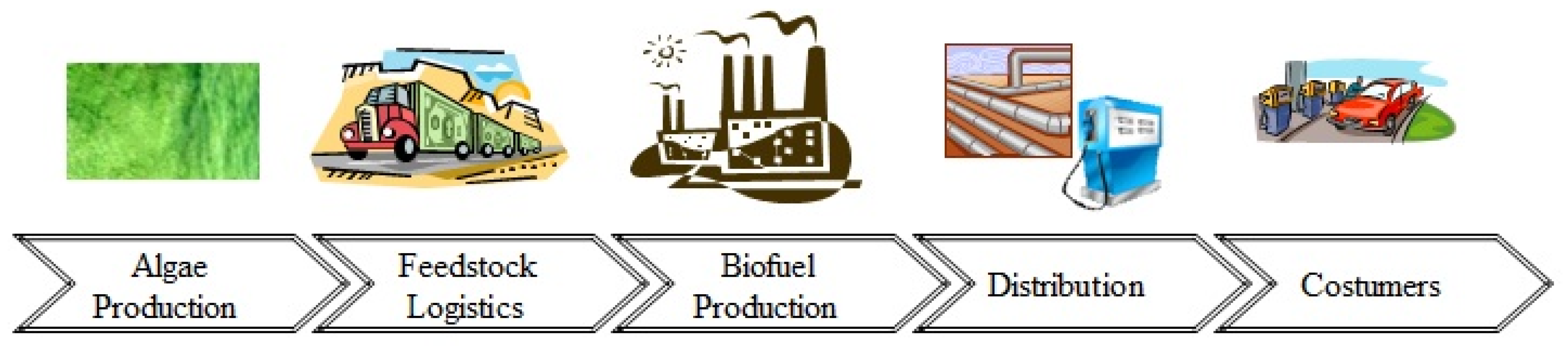
2. Problem Statement and Algae Supply Chain Description

Givens are a particular algae species, cultivation (supply) locations, demand locations, and known demand requirements at those demand locations. The goal is to design a supply chain network that distributes the necessary algae biomass from supply locations to meet biodiesel demand at specified demand locations. The final supply chain topology includes the optimum sites to grow the biomass, to extract the algae oil from algae biomass, and to convert the algae oil into biodiesel. The model also determines the optimum open pond size and geometry for each biomass cultivation site. The objective is to minimize the overall cost of the supply chain, including production, operating, and transportation costs over a planning horizon of ten years.

The algal biomass to biodiesel supply chain contains algae production, feedstock logistics, biodiesel production, distribution, and customers (Figure 1). Algae biomass production depends on algae species, geographical location, and cultivation technology selected for culturing. The cultured biomass is harvested, dried, and undergoes extraction to produce algae oil, which is sent to a biofuel production facility where biodiesel is produced. Feedstock logistics is the supply chain between feedstock (algae) production and conversion (biodiesel). It includes harvesting, processing, transport and storage of the products at different stages of biodiesel production. The produced biodiesel is dispatched to distribution centers, and from there, it reaches the consumers.

The model is presented in the next section. Algae production at supply locations is modeled using the pond model of Yadala [8]. This model is then integrated with feedstock logistics, where the produced algae biomass from supply locations is transported to algae oil extraction facilities, and afterward to distribution centers (i.e., demand locations) via biofuel production facilities (i.e., transesterification locations). In this approach, in addition to regional economics, such as land, labor, water, and electricity costs, distances between different operating locations and their associated costs are considered. The method aids in the calculation of production, operating, and transportation costs more accurately.

3. Mathematical Programming Model

The goal of the algal biomass to biodiesel supply chain network is to meet the specific biodiesel demands of a set of locations with minimum overall cost. The formulation determines the best locations for algae production, algal oil extraction, and biodiesel production given potential algal farming sites, oil extraction locations, and biodiesel production sites along with the optimum number of algae ponds and their design specifications. A detailed listing of sets, parameters, variables included in the formulation is compiled in the nomenclature section at the end of the document. A brief summary of the sets and a detailed overview of the formulation are discussed below.

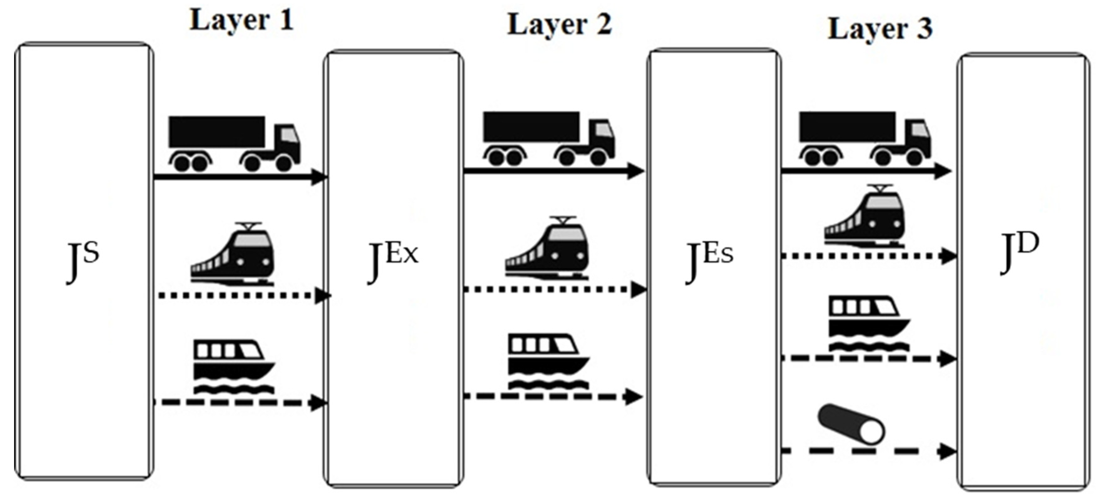
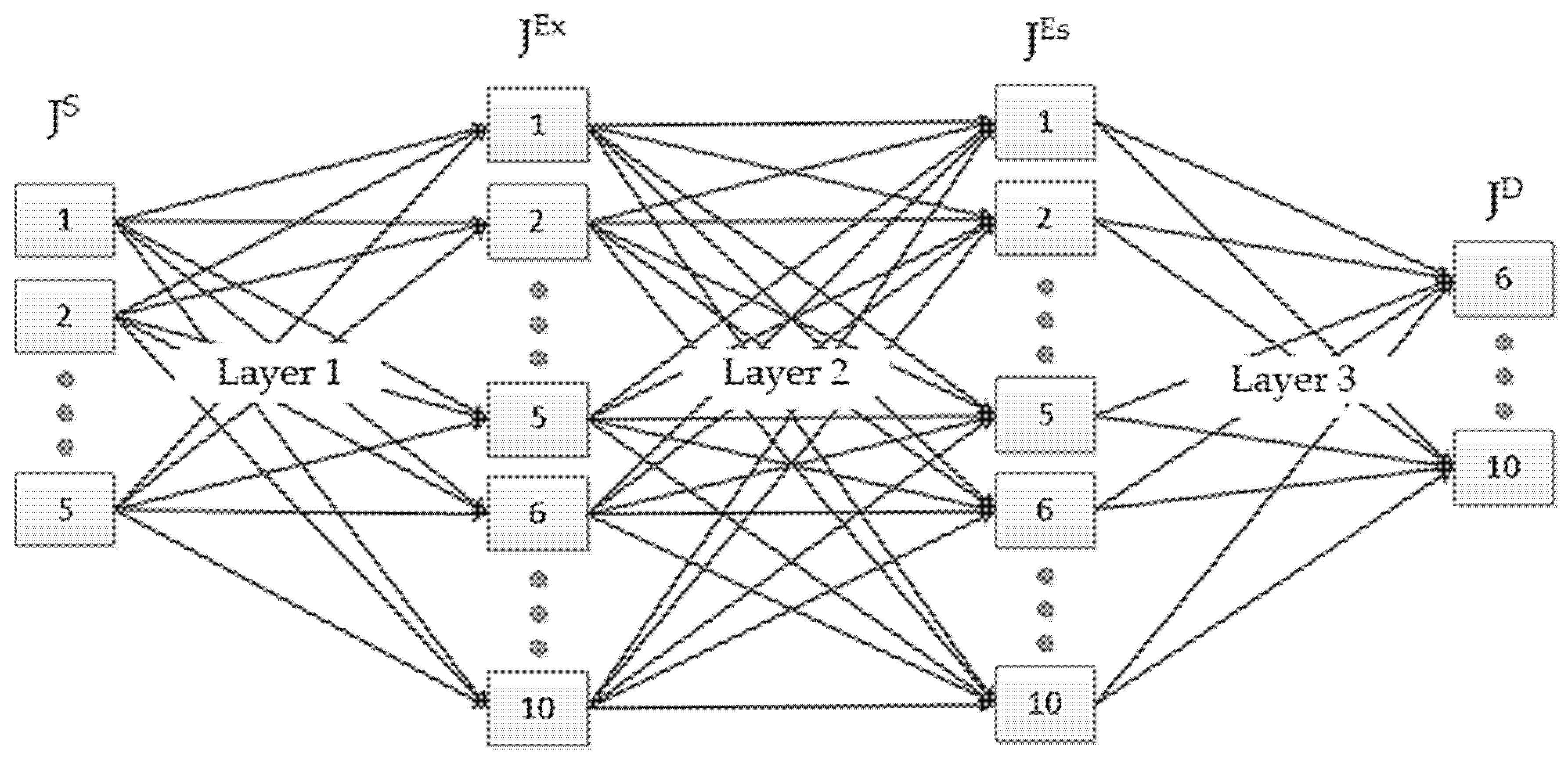
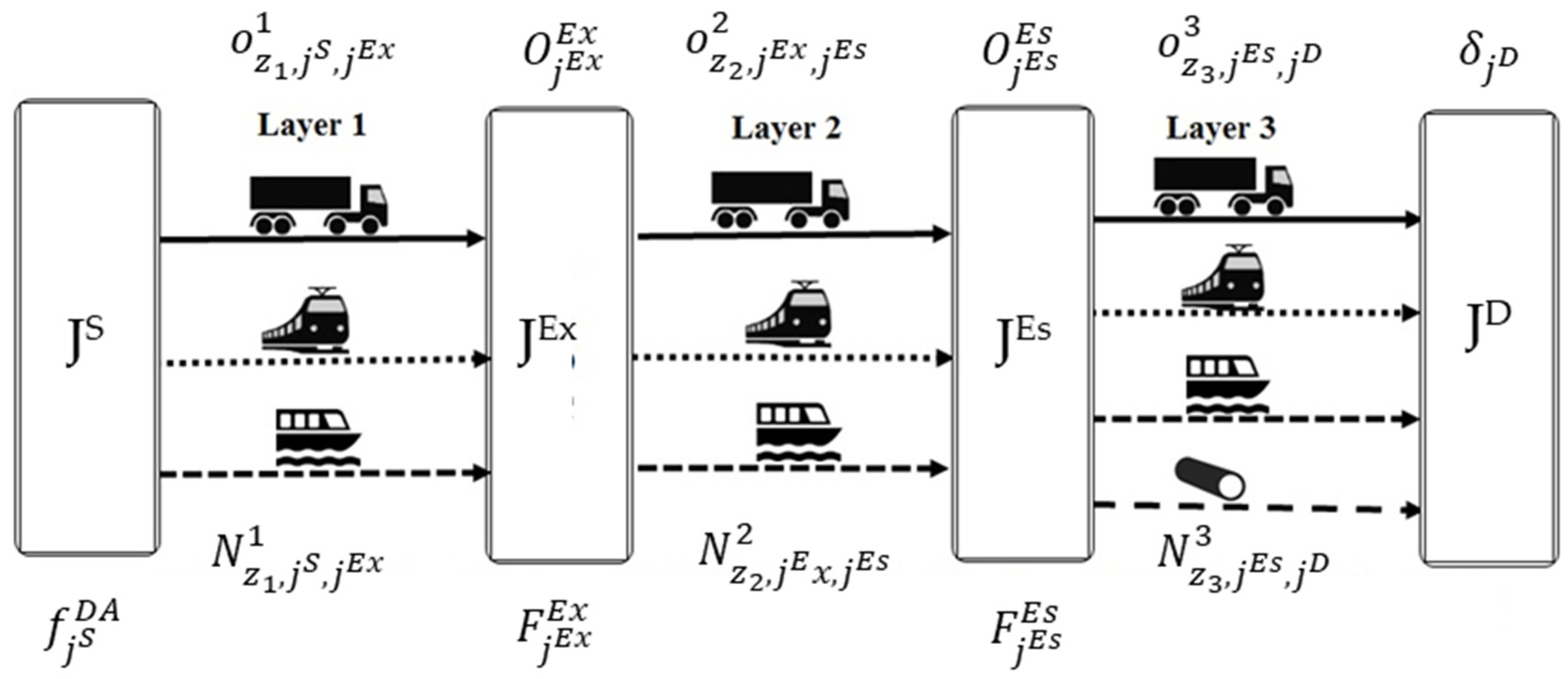
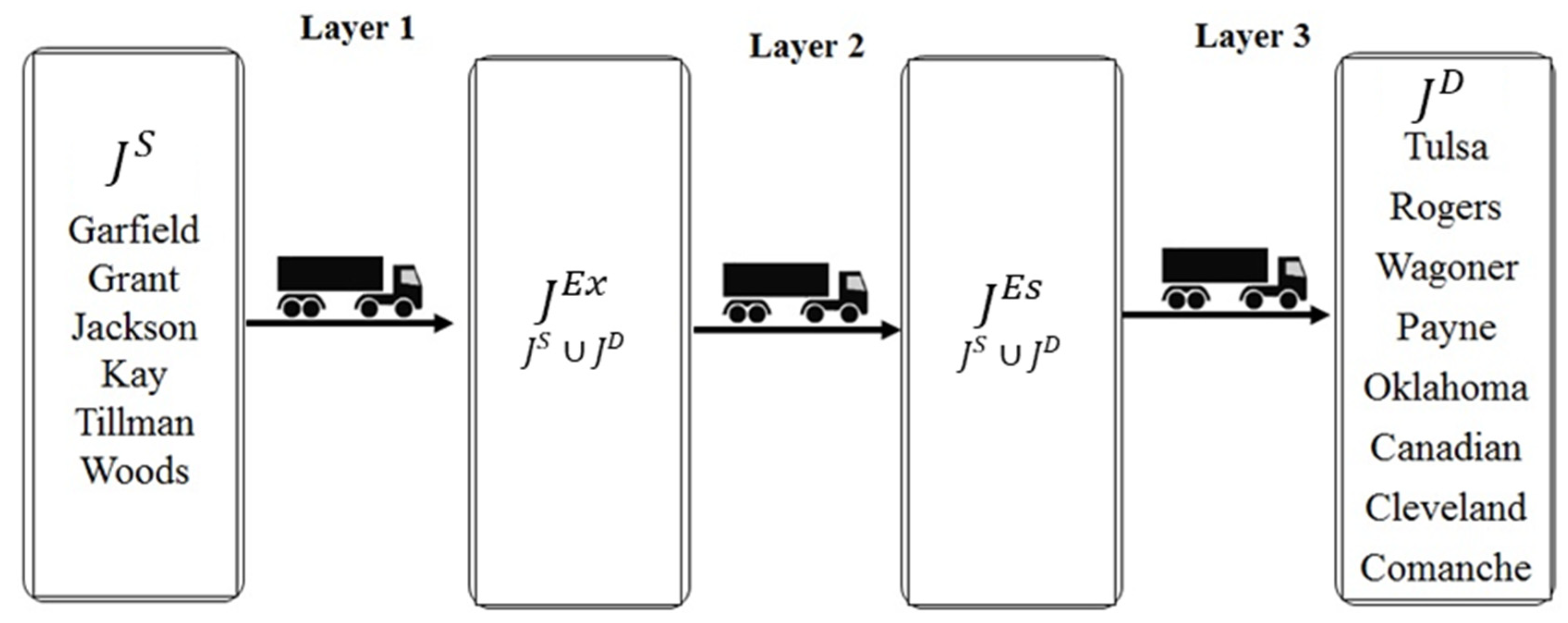
3.1. Geographical and Network Sets

The first data set in this multi-echelon supply chain model defines all candidate locations where facilities can be placed, $J$. From this set, subsets are constructed to correspond to the different operations within the supply chain. Subset $J^S$ corresponds to the candidate supply locations for the production of algal biomass. The supply portion of the model is designated by a superscript of $S$ for model variables and parameters. Subset $J^{Ex}$ is constructed of the candidate locations for the extraction of algal oil from the dried biomass. Model variables and parameters pertaining to the extraction operation are indicated by the use of superscript $Ex$. The third operation within the supply chain, the transesterification of algal oil to biodiesel, is described by the superscript $Es$. For the potential locations for these operations the subset $J^{Es}$ is used. Finally, the locations of demand are included in subset $J^D$, with variables and parameters associated with the demand denoted by a superscript $D$. The defined subsets are not mutually exclusive as some locations may appear in multiple subsets.

The supply chain model has four echelons, and hence, three layers, $i\in I=\left\{1,2,3\right\}$, that material can be transported from one echelon to the next. Layer 1, connects the supply locations,$J^S$, to the extraction locations, $J^{Ex}$. Layer 2 connects extraction locations to the sites where the transesterification occurs, $J^{Es}$. The final layer, layer 3, connects the transesterification locations to the demand locations, $J^D$. There are a number of transportation modes, $z\in Z=\left[\mathrm{trucks},\mathrm{rail}\mathrm{cars},\mathrm{barges},\mathrm{pipeline}\right]$, that can be used for moving materials between echelons in each layer. The transportation modes associated with each layer, are created through the subsets $z_i\in Z_i\subset Z$, where $i$ corresponds to the layer. Figure 2 demonstrates the interplay of the supply chain operation locations, transportation layers, and the modes of transportations for each layer. The sets of dates, $d\in D$, and time of the day,$t\in T$, enable tracking the parameters relevant to the growth of algae biomass that is date and time of day dependent, e.g., length of the light path or the solar irradiance.

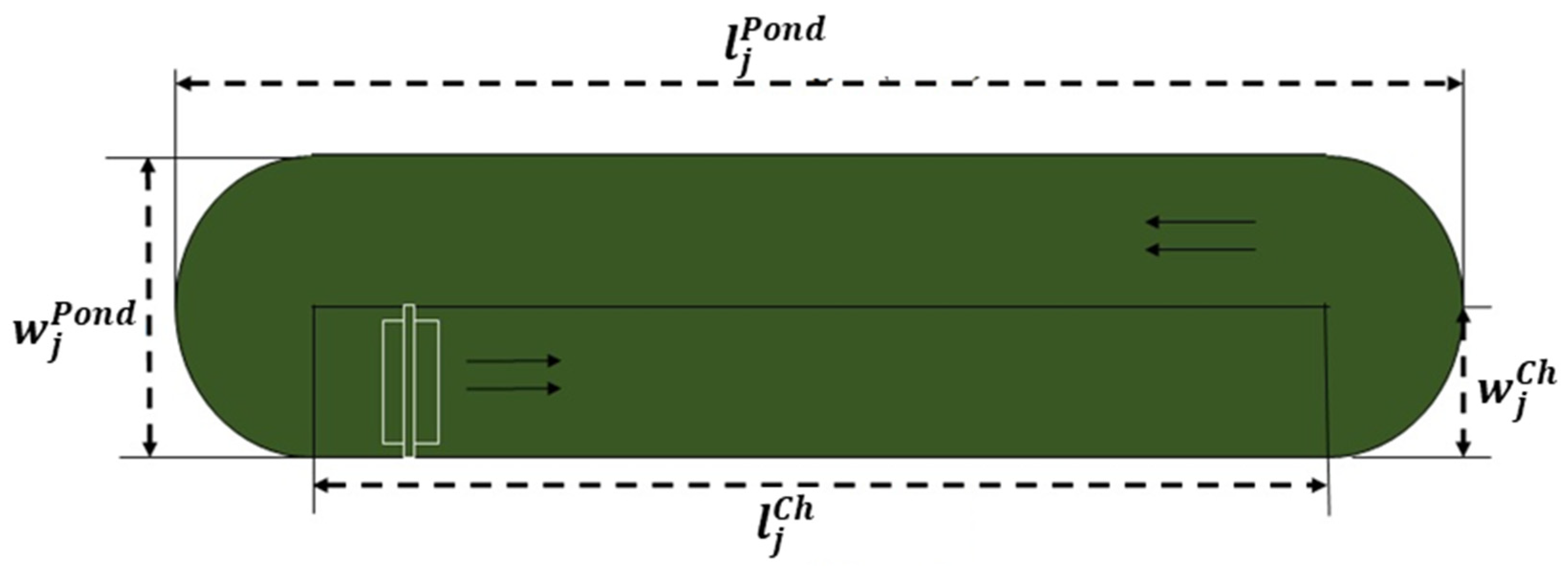
3.2. Constraints Related to Supply Sites

At the supply locations, algae biomass is produced in outdoor open channel raceway ponds under the influence of sunlight and temperature fluctuations. To reduce computational burden when running the integrated pond model year long between sunrise and sunset, a simplified approach was followed. All available weather data within each month was approximated to one specific day of that month. This decreased the number of days from 360 to 12 days in a dynamic pond model. The variables obtained for that one specific day of the month are replicated for all other days in that month. Additional information on pond modeling can be obtained from Yadala [8] and a summary of the model provided in Appendix B of this paper. These constraints are used to calculate the dry algae biomass produced in a year from a single pond at a supply location $j\in J^S$, given by the variable $f_j^{DA}$. Equations (1)–(6) below are the constraints related to the pond geometry. They are taken from the pond model and are integrated with the supply chain model.

$$w_j^{Pond}=2w_j^{Ch} \forall j\in J^S,$$

(1)

$$\frac{l_j^{Ch}}{w_j^P}\ge 10 \forall j\in J^S,$$

(2)

$$l_j^{Pond}=l_j^{Ch}+w_j^{Pond} \forall j\in J^S,$$

(3)

$$l_j^{Pond}\le 300 m \forall j\in J^S ,$$

(4)

$$A_j^{Pond}=\frac{\pi {\left(w_{j^S}^{Pond}\right)}^2}{4}+l_j^{Ch}{w}_j^{Pond} \forall j\in J^S,$$

(5)

$$V_j^{Pond}=A_j^{Pond}{h}_j^{Pond} \forall j\in J^S.$$

(6)

Equation (1) requires that for a single-channel raceway pond, total pond width, $w_j^{Pond}$, is twice the channel width, $w_j^{Ch}$. To avoid the flow disturbance caused by the bends of the raceway pond, the ratio of channel length to width should be ten or higher [23] (Equation (2)). Pond length, $l_j^{Pond}$, is the summation of channel length and pond width (Equation (3)). Pond length is constrained to keep the head loss due to friction (Equation A20) lower via Equation (4). The surface area occupied by the pond, $A_j^{Pond}$, is computed from Equation (5). Finally, Equation (6) calculates the volume of the raceway pond, $V_j^{Pond}$. Figure 3 provides a physical representation of the various measurements associated with the raceway pond.

It is assumed that the size of a single pond does not change within each supply location and that it may be necessary to have more than one pond in each supply location to meet the demand. Total surface area, $A_j^{Tot}$, occupied by the ponds at each supply location is calculated by multiplying the number of ponds,$N_j^{Pond}$, with the surface area of a single pond at the supply location, according to (Equation (7)). This is done, as it is assumed that every pond at one location shares the same dimensions. The variable $A_j^{Tot}$ cannot exceed the marginal farmland available, ${\mathsf{\Lambda }}_j^{Tot}$, in that region (Equation (8)). Equation (9) ensures that the surface area of a single raceway pond does not exceed the maximum allowable single pond area at that location, ${\mathsf{\Lambda }}_j^{Pond}$. Equation (10) ensures that when there are no ponds at any supply location, the surface area would be zero.

$$A_j^{Tot}=N_j^{Pond}{A}_j^{Pond} \forall j\in J^S,$$

(7)

$$A_j^{Tot}\le {\Lambda }_j^{Tot} \forall j\in J^S,$$

(8)

$$A_j^{Pond}\le {\Lambda }_j^{Pond} \forall j\in J^S,$$

(9)

$$A_j^{Pond}\le N_j^{Pond}{\Lambda }_j^{Pond} \forall j\in J^S.$$

(10)

The sum of all the shipment, $o_{z,j^S,j^{Ex}}^1$, via any method of transportation, $z\in Z_1$, from a supply location, $j^S\in J^S$, to all extraction facilities, $j^{Ex}\in J^{Ex}$, in transportation layer 1 should not exceed the total dry algae production at a supply location, which is obtained by multiplying the dry algae biomass, DA, produced in a year from a single pond, $f_{j^S}^{DA}$, with the number of such ponds at the location, viz. Equation (11). The total amount of dry algae shipped from all supply locations, $j^S\in J^S$, to an extraction facility via any method of transportation, is defined as the dry algae being transported to, $O_{j^{Ex}}^{Ex}$, and is calculated using Equation (12).

$${\sum }_{j^{Ex}\in J^{Ex}}{\sum }_{z\in Z_1}{o}_{z,j^S,j^{Ex}}^1\le N_{j^S}^{Pond}{f}_{j^S}^{DA} \forall j^S\in J^S,$$

(11)

$${\sum }_{j^S\in J^S}{\sum }_{z\in Z_1}{o}_{z,j^S,j^{Ex}}^1=O_{j^{Ex}}^{Ex} \forall j^{Ex}\in J^{Ex}.$$

(12)

3.3. Constraints Related to Distribution Sites

These constraints are written for extraction locations, $j^{Ex}\in J^{Ex}$, and transesterification locations, $j^{Es}\in J^{Es}$, and they correspond to the second transportation layer of the model. Algae oil is extracted from the biomass at extraction locations, and it is converted to biodiesel via transesterification at transesterification locations.

At an extraction facility, $j\in J^{Ex}$, depending on the extraction efficiency, ${\eta }^{Ex}$, and oil content of the algae species, ${\mathsf{\Psi }}_s$, the amount of algae oil produced, $F_j^{Ex}$, is calculated with Equation (13). The total amount of algae oil shipped, $o_{z,j^{Ex},j^{Es}}^2$, from an extraction facility, $j^{Ex}\in J^{Ex}$, to various transesterification facilities, $j^{Es}\in J^{Es}$, via any method of transportation, $z\in Z_2$, cannot exceed the total algae oil extracted,$F_{j^{Ex}}^{Ex},$ at $j^{Ex}\in J^{Ex}$ (Equation (14)). The total amount of algae oil shipped from all extraction facilities,$j^{Ex}\in J^{Ex}$, to a transesterification facility, $j^{ES}\in J^{ES}$, is equal to algae oil transported to transesterification location, $O_{j^{Es}}^{Es}$, as shown in Equation (15).

$$F_j^{Ex}={\eta }^{Ex}{\mathsf{\Psi }}_s{O}_j^{Ex} \forall j\in J^{Ex},$$

(13)

$${\sum }_{j^{Es}\in J^{Es}}{\sum }_{z\in Z_2}{o}_{z,j^{Ex},j^{Es}}^2\le F_{j^{Ex}}^{Ex} \forall j^{Ex}\in J^{Ex},$$

(14)

$${\sum }_{j^{Ex}\in J^{Ex}}{\sum }_{z\in Z_2}{o}_{z,j^{Ex},j^{Es}}^2=O_{j^{Es}}^{Es} \forall j^{Es}\in J^{Es} ,$$

(15)

At the transesterification facilities, biodiesel is produced via a transesterification reaction, which is given in Equation (16). For this model, the overall yield of the transesterification process is defined using transesterification efficiency, ${\eta }^{Es}$. The transesterification efficiency, which by definition should be between zero and one, is the efficiency of conversion of algae oil to biodiesel. The amount of biodiesel produced, $F_j^{Es},$ at transesterification location $j\in J^{Es}$, can be calculated using Equation (16). Here, $M{W}_{biodiesel}$ is the molecular weight of biodiesel [24] and $M{W}_{lipid}$ is the molecular weight of lipids [25]. Equation (17) shows that the total amount of shipment, $o_{z,j^{Es},j^D}^3$, from a transesterification facility $j^{Es}\in J^{Es}$, to all demand locations, $j^D\in J^D$, via any method of transportation cannot exceed the biodiesel produced at a transesterification location, $F_{j^{Es}}^{Es}$.

$$F_j^{Es}=3{\eta }^{Es}\left(\frac{M{W}_{biodiesel}}{M{W}_{lipid}}\right)O_j^{Es} \forall j\in J^{Es},$$

(16)

$${\sum }_{j^D\in J^D}{\sum }_{z\in Z_3}{o}_{z,j^{Es},j^D}^3\le F_{j^{Es}}^{Es} \forall j^{Es}\in J^{Es}.$$

(17)

3.4. Constraints Related to Demand Locations

The total amount of biodiesel shipped from all transesterification facilities meets the demand, ${\delta }_{j^D}$ at demand location $j^D\in J^D$. Equation (18) ensures that biodiesel demand at each demand location is satisfied.

$${\sum }_{j^{Es}\in J^{Es}}{\sum }_{z\in Z_3}{o}_{z,j^{Es},j^D}^3\ge {\delta }_{j^D} \forall j^D\in J^D.$$

(18)

Figure 4 shows the network flow topology of the model. Here, $J^S$ represents the algae biomass production or supply locations labeled as 1 through 5. $J^{Ex}$ represents extraction sites where algae oil is extracted. $J^{Es}$ represents transesterification sites where biodiesel is produced. The $J^{Ex}$ and $J^{Es}$ considers both supply and demand locations together to include all possible combinations of locations. $J^D$ represents demand locations of biodiesel.

3.5. Constraints Related to Transportation

Different materials are shipped through each layer of arcs in Figure 4. For example, dry algae biomass, $o_{z,j^S,j^{Ex}}^1$, is shipped from supply locations to extraction locations through layer one. The algae oil, $o_{z,j^{Ex},j^{Es}}^2$, from extraction facilities is shipped to transesterification facilities in layer two. Finally, biodiesel, $o_{z,j^{Es},j^D}^3$, from transesterification facilities is shipped to demand locations through layer three. Two different means of transportation are considered for each layer, shipment via land or water. The number of such transportation methods, ($N_{z,j^{Source},j^{Sink}}^i$), required to ship the products between each layer depends on the capacity, ${\mathsf{\Xi }}_{z_i}$, of the method, $z_i\in Z_i$, for layer $i\in I$, and density of the product being shipped. These relationships are enforced via Equations (19)–(21).

$$N_{z,j^S,j^{Ex}}^1=\frac{o_{z,j^S,j^{Ex}}^1}{\left({\mathsf{\Xi }}_z{\rho }^{DryAlgae}\right)} \forall z\in Z_1,\forall j^S\in J^S, \forall j^{Ex}\in J^{Ex},$$

(19)

$$N_{z,j^{E}x,j^{Es}}^2=\frac{o_{z,j^{Ex},j^{Es}}^2}{\left({\mathsf{\Xi }}_z{\rho }^{AlgaeOil}\right)} \forall z\in Z_2,\forall j^{Ex}\in J^{Ex}, \forall j^{Es}\in J^{Es},$$

(20)

$$N_{z,j^{Es},j^D}^3=\frac{o_{z,j^{Es},j^D}^3}{\left({\mathsf{\Xi }}_z{\rho }^{Biodeisel}\right)} \forall z\in K_3,\forall j^{Es}\in J^{Es}, \forall j^D\in J^D .$$

(21)

Here, ${\rho }^{DryAlgae}$, ${\rho }^{AlgaeOil}$, and, ${\rho }^{Biodiesel}$ are the densities of dry algae biomass (kt m⁻³), algae oil (kt m⁻³), and biodiesel (kt m⁻³), respectively. The entire supply chain network and the related variables associated with it are depicted in Figure 5.

3.6. Objective Function

The objective is to minimize the overall cost, $TC$, of biodiesel supply chain network, presented in Equation (22).

$$TC=C{C}^S+C{C}^{Ex}+C{C}^{Es}+{\sum }_{y\in Y}\frac{1}{{\left(1+MARR\right)}^i}\left[MC+WC+LC+PC+O{C}^S+O{C}^{Ex}+O{C}^{Es}+TrC\right].$$

(22)

The Minimum Acceptable Rate of Return (MARR) is 15%. Here, $C{C}^S$ and $O{C}^S$ are the capital and operating costs of raceway pond. They are calculated, scaling linearly, depending on the total surface area of the pond through Equations (23) and (24),

$$C{C}^S={\xi }^C{\sum }_{j\in J^S}{A}_j^{Tot},$$

(23)

$$O{C}^S={\xi }^O{\sum }_{j\in J^S}{A}_j^{Tot},$$

(24)

where, ${\xi }^C$ is the total capital investment, and ${\xi }^O$ is the total product cost per pond area (which are given in Yadala [8]).

Capital and operating costs, $C{C}^{Ex}$ and $O{C}^{Ex}$, for extraction of algae oil are assumed to change linearly with the total oil production at a site, and are estimated by Equations (25) and (26), where, ${\psi }^{C,Ex}$ and ${\psi }^{O,Ex}$ are the capital and operating cost coefficients for the selected algal oil extraction process.

$$C{C}^{Ex}={\sum }_{j\in J^{Ex}}\left({\psi }^{C,Ex}{F}_j^{Ex}\right),$$

(25)

$$O{C}^{Ex}={\sum }_{j\in J^{Ex}}\left({\psi }^{O,Ex}{F}_j^{Ex}\right).$$

(26)

Assuming capital and operating costs, $C{C}^{Es}$ and $O{C}^{Es}$, for transesterification of biodiesel changes linearly with the amount of biodiesel produced at a location, these costs are calculated using Equations (27) and (28).

$$C{C}^{Es}={\sum }_{j\in J^{Es}}\left({\psi }^{C,Es}{F}_j^{Es}\right),$$

(27)

$$O{C}^{Es}={\sum }_{j\in J^{Es}}\left({\psi }^{O,Es}{F}_j^{Es}\right) .$$

(28)

Here, ${\psi }^{C,Es}$ and ${\psi }^{O,Es}$ are the capital and operating cost coefficients for the selected transesterification process.

Land cost, $LC$, considers the purchase (or lease) cost, ${\chi }_j^{Land}$, of the required land area for algae cultivation, and only considers the required surface area for the ponds at location $j\in J^S$. It is calculated using Equation (29). Water cost, $WC$, is calculated based on the total amount of industrial water, $V_j^{Ind}$, required for algal cultivation in a single pond, number of such ponds, and the utility cost of water, ${\chi }_j^{Water}$, at supply location $j\in J^S$. This is shown in Equation (30). $V_j^{Ind}$ in Equation (30) is calculated using Equation (A57) in Appendix B.

$$LC={\sum }_{j\in J^S}\left({\chi }_j^{Land}{A}_j^{Tot}\right),$$

(29)

$$WC={\sum }_{j\in J^S}\left({\chi }_j^{Water}{N}_j^{Pond}{V}_j^{Ind}\right).$$

(30)

Mixing and pumping costs, $MC$ and PC, associated with raceway pond are estimated from Equations (31) and (33) using total energy required for mixing and pumping, and electric cost, ${\chi }_j^{Elect}$, at the respective supply location $j\in J^S$. Total mixing and pumping energy are calculated from the total power requirements for all ponds at the supply location (Equations (32)–(34)). In Equation (32), the power required by paddle wheel of raceway pond, $P{W}_{j,d,t}$, for location $j\in J^S$ for all representative days $d\in D$ for all times of day $t\in T$, is calculated from Equation (A43) in Appendix B. In Equation (34), the power required by pumps in raceway pond, $P{P}_{j,d,t}$, for location $j\in J^S$ for all representative days $d\in D$ for all times of day $t\in T$, is calculated using Equation (A44) in Appendix B.

$$MC={\sum }_{j\in J^S}{\chi }_j^{Elect}EM,$$

(31)

$$E{M}_j=30{\sum }_{d\in D}{\sum }_{,t\in T}\left(N_j^{Pond}P{W}_{j,d,t}\right) \forall j\in J^S,$$

(32)

$$PC={\sum }_{j\in J^S}{\chi }_j^{Elect}E{P}_j,$$

(33)

$$E{P}_j=30{\sum }_{d\in D}{\sum }_{t\in T}\left(N_j^{Pond}P{P}_{j,d,t}\right) \forall j\in J^S.$$

(34)

Transportation cost, $TrC$, for the shipment of dry algae, algae oil, and biodiesel that are associated with the first, second, and third layers of the supply chain network is detailed in Equation (35). The costs for each transportation layer are the product of the distance, ${\gamma }_{z_i,j^{Source},j^{Sink}}$, from the source location, $j^{Source}\in J$, to the sink location, $j^{Sink}\in J$, using transportation mode $z_i\in Z_i$, and the cost per distance, ${\varphi }_{i,z_i}$, to use transportation mode $z_i\in Z_i$ for all the transportation layers $i\in I$.

$$\begin{gathered} TrC={\sum }_{z_1\in Z_1}{\sum }_{j^S\in J^{\mathrm{S}}}{\sum }_{j^{Ex}\in J^{Ex}}\left({\varphi }_{1,z_1}{\gamma }_{z_1,j^{\mathrm{s}},j^{Ex}}{N}_{Z_1,j^{\mathrm{s}},j^{Ex}}^1\right)+ \\ {\sum }_{z_2\in Z_2}{\sum }_{j^{Ex}\in J^{Ex}}{\sum }_{j^{Es}\in J^{Es}}\left({\varphi }_{2,z_2}{\gamma }_{z_2,j^{Ex}{j}^{Es}}{N}_{Z_2,j^{Ex}{j}^{Es}}^2\right)+ \\ {\sum }_{z_3\in K_3}{\sum }_{j^{Es}\in J^{Es}}{\sum }_{j^D\in J^D}\left({\varphi }_{3,z_3}{\mu }_{z_3,j^{Es}{j}^D}{N}_{Z_3,j^{Es}{j}^D}^3\right). \end{gathered}$$

(35)

4. Case Studies

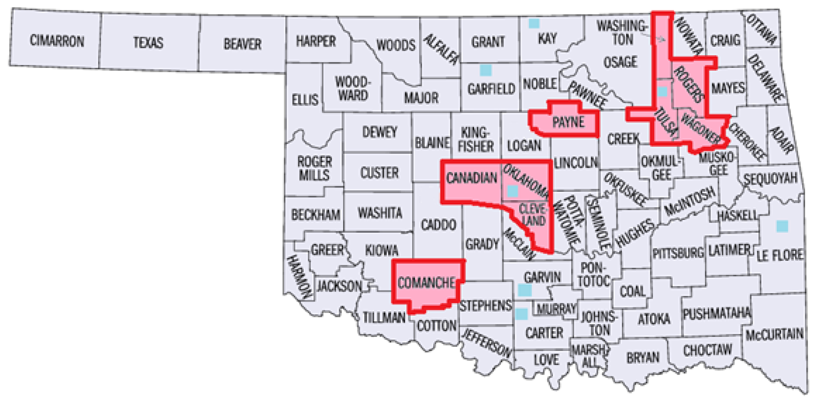
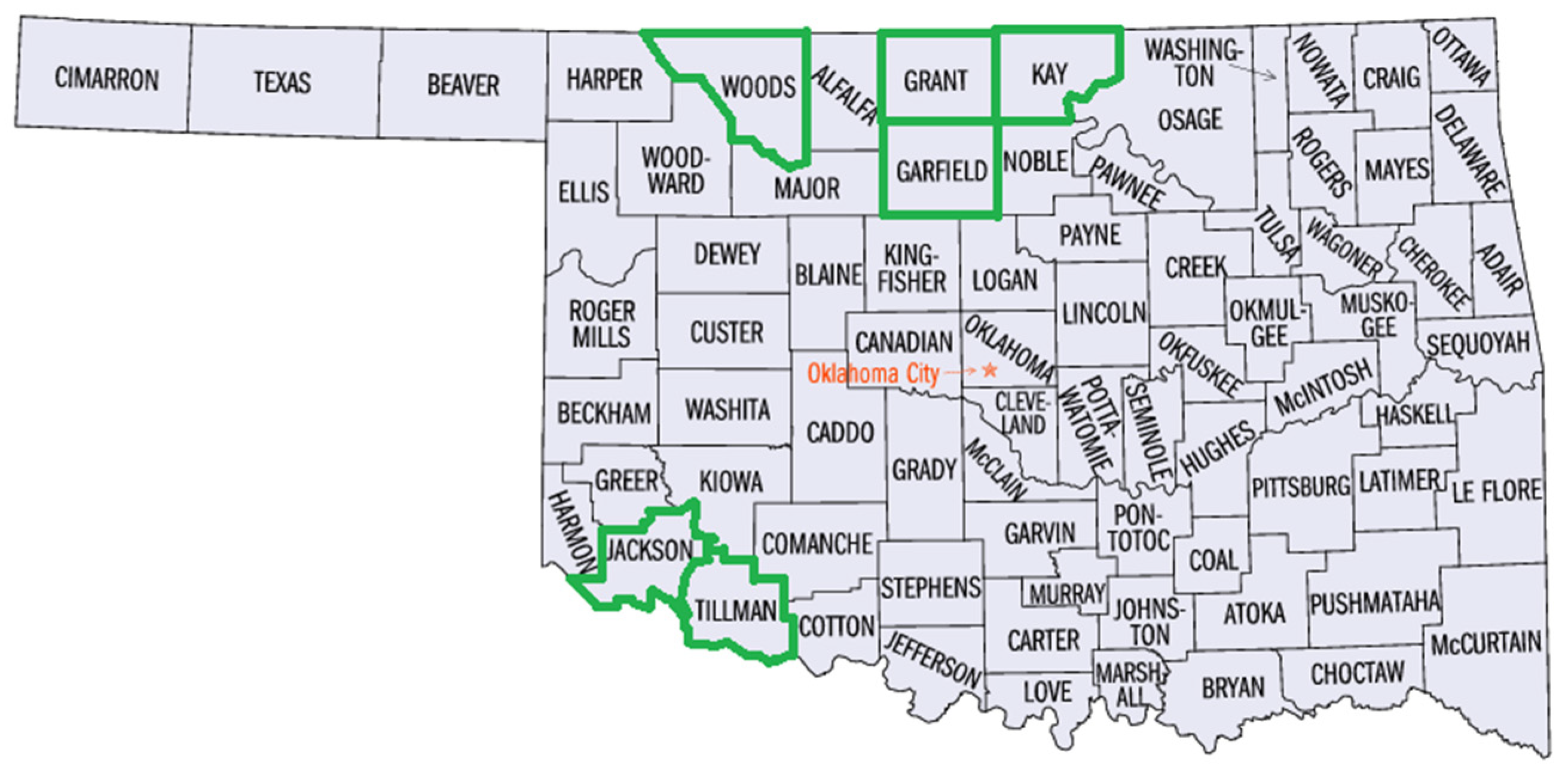
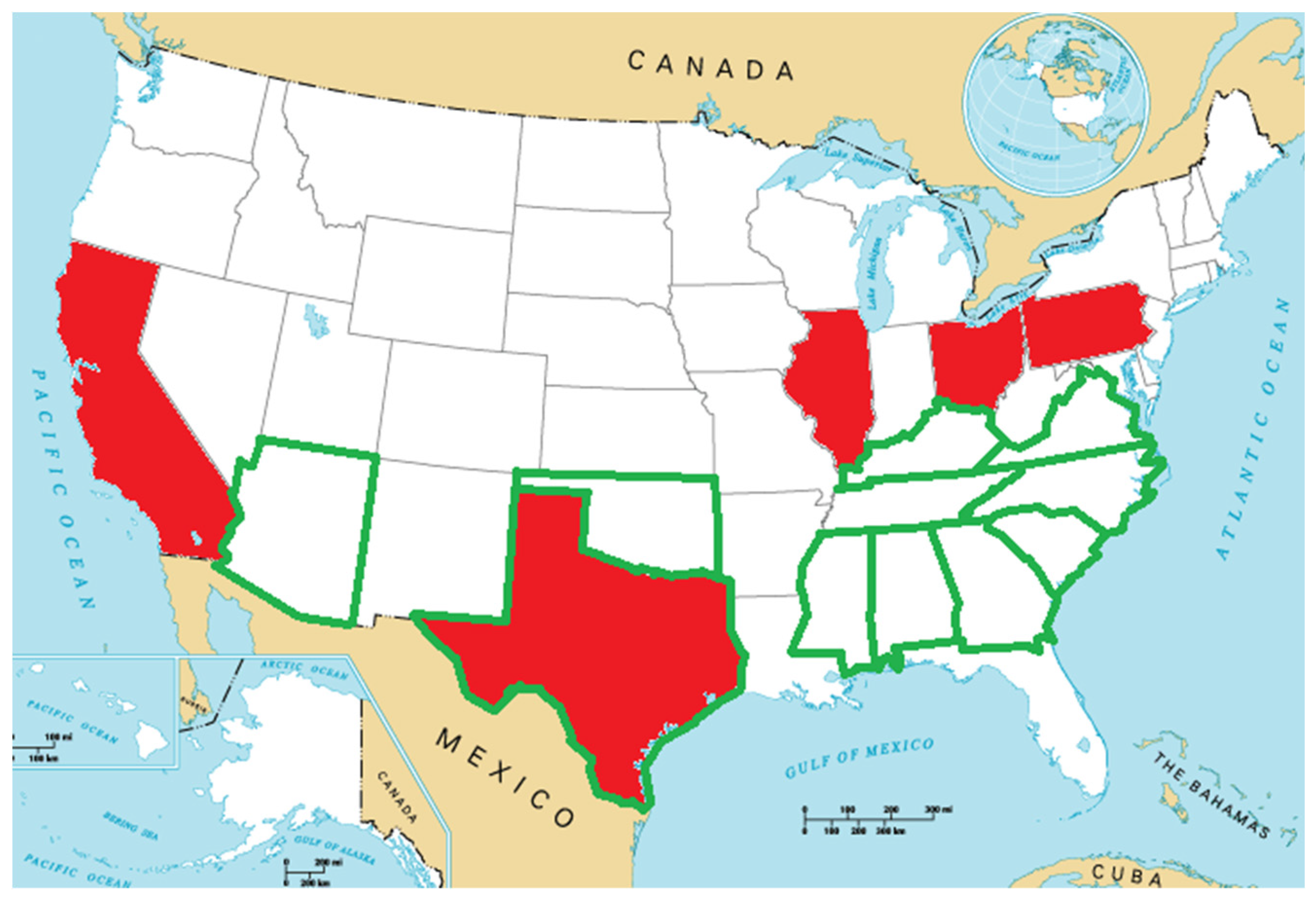
4.1. State of Oklahoma

The first case examined is the supply chain network for algae biodiesel production in the counties of the state of Oklahoma (Figure 6). The algae species, I. galbana is chosen for use within the raceway style ponds dues to their allowance of higher light absorption withing the pond, which drives down costs [8]. The demand and supply locations for the state are identified using several criteria.

The counties were first eliminated as potential demand centers based on population density at 100 persons/mi² (38.6 persons/km²). This cutoff is selected because there is a sudden jump in population densities from 90.34 people/mi² to 115.48 people/mi². Combined, the nine remaining counties, shown in pink in Figure 7, account for more than 56% of the population of the entire state. The number of demand locations may be further reduced by looking at how fuel terminals are currently spread throughout the state. In Figure 7, these are shown as counties with solid blue squares. Because of this, the demand counties are grouped into regions that may each be served by a single terminal, e.g., counties in a metropolitan area can be served by the central city. For example, we assume that biodiesel deliveries for the Tulsa, Washington, Rogers, and Wagoner county region will be delivered to the final supplier in Tulsa County, the location of the principal regional city. The fuel demand of the reduced regions is presented in

Table 1. Population and diesel consumption for demand regions and for the entire state of Oklahoma, along with estimated biodiesel demand fulfillment capacity.

$\mathbf{Demand}\mathbf{Regions}\left({\mathit{J}}^{\mathit{D}}\right)$	Population	Total Diesel Demand (U.S. Gallons)	Biodiesel Demand	Biodiesel Demand
			25% of Diesel Demand	25% of Diesel Demand
			(U.S. Gallons)	(Million Liters)
Tulsa, Rogers, Wagoner	829,612	3.269 × 108	8.17 × 107	309.37
Payne	78,479	3.092 × 107	7.73 × 106	421.90
Oklahoma, Canadian, Cleveland	1,131,362	4.458 × 108	1.12 × 108	47.22
Comanche	126,611	4.989 × 107	1.25 × 107	29.27

The supply locations for growing algae biomass is determined based on two criteria. The first is the amount of marginal farmland in each county. We first define total county farmland using the United States Department of Agriculture (USDA) National Agricultural Statistics Service (NASS) 2012 Census of Agriculture statistic ‘Land in farms’ found within the report [27]. We further define marginal cropland as per Equation (36).

$$\begin{array}{c}Croplan{d}_{marginal}{=Cropland}_{Total}-{Cropland}_{Harvested}-{Cropland}_{Other,Total}+\\ {Cropland}_{Other,Idle}+{Cropland}_{Other,Failed}.\end{array}$$

(36)

In Equation (36), each variable corresponds to the same-named column in the 2012 Census of Agriculture. In-use cropland is then defined as the total cropland minus the marginal cropland. Using this definition, the total county marginal farmland can be defined per Equation (37),

$$Farmlan{d}_{marginal}=Farmlan{d}_{Total}-Croplan{d}_{In-use}-Pastureland-Lan{d}_{Buildings,roads,ponds},$$

(37)

where, again, other than $Croplan{d}_{In-use}$ and $Farmlan{d}_{Marginal}$, each variable corresponds to the same-named column in the 2012 Census of Agriculture. All 77 counties of Oklahoma are ranked in descending order according to the amount of marginal farmland.

The second criterion eliminates counties based on the average well depth in each county, arising from the assumption that water will be obtained through wells in this case study. In Oklahoma, whenever a well is dug, it is required that well logs be submitted to the Oklahoma Water Resource Board within sixty days [28]. These records are collected and digitized within the groundwater well data set [29]. After removing wells not in the irrigation, commercial, industrial, or public water supply categories (i.e., those used for home water supplies which do not require as much drawdown as wells with higher flow rates), the average well depth for each county was calculated, and counties were ranked in ascending order from shallowest to deepest. Those counties ranking in the top 25% for both measures were taken as the set of supply counties, outlined in green in Figure 8. The available marginal farmland in each of these counties is given in

Table 2. Marginal farmland and average agricultural land cost for counties considered as potential suppliers of algal biomass. [27,29].

Supply Locations $\left({\mathit{J}}^{\mathit{S}}\right)$	Available Land (km2)	Land Cost ($/km2)
Garfield	156.2	42000
Grant	318.0	33000
Jackson	244.2	28700
Kay	163.5	40400
Tillman	180.1	30700

, along with the cost of land in each [30]. The average cost of electricity for 2013 was 5.43 cents/kWh [31], while the average energy cost for irrigation water was 1.97 cents/1000 U.S. gallons [27].

All of the supply centers and demand regions were assumed to be available for the two remaining steps in the algae biomass to biodiesel supply chain, oil extraction, and transesterification. Taken together, a supply chain network as shown in Figure 9 was created.

The mode of transportation considered between all layers for this case is trucks. The capacity of the truck, ${\mathsf{\Xi }}_{truck}$, is taken as 30 m³ [32]. All the distances between supply, extraction, transesterification, and demand locations are given in Appendix A in

Table A1. Road distances between all locations, Oklahoma case.

	Garfield	Grant	Jackson	Kay	Tillman	Woods	Tulsa	Oklahoma	Comanche	Payne
Garfield	0	32.8	211	63.2	194	83.2	121	94	144	68.5
Grant	32.8	0	249	31.5	231	70	137	110	176	84.4
Jackson	211	249	0	257	49.1	178	258	166	66.3	216
Kay	63.2	31.5	257	0	238	98.3	110	99.8	190	57
Tillman	194	231	49.1	238	0	176	243	148	49.9	198
Woods	83.2	70	178	98.3	176	0	205	177	179	151
Tulsa	121	137	258	110	243	205	0	101	191	74.1
Oklahoma	94	110	166	99.8	148	177	101	0	100	59.2
Comanche	144	176	66.3	190	49.9	179	191	100	0	150
Payne	68.5	84.4	216	57	198	151	74.1	59.2	150	0

.

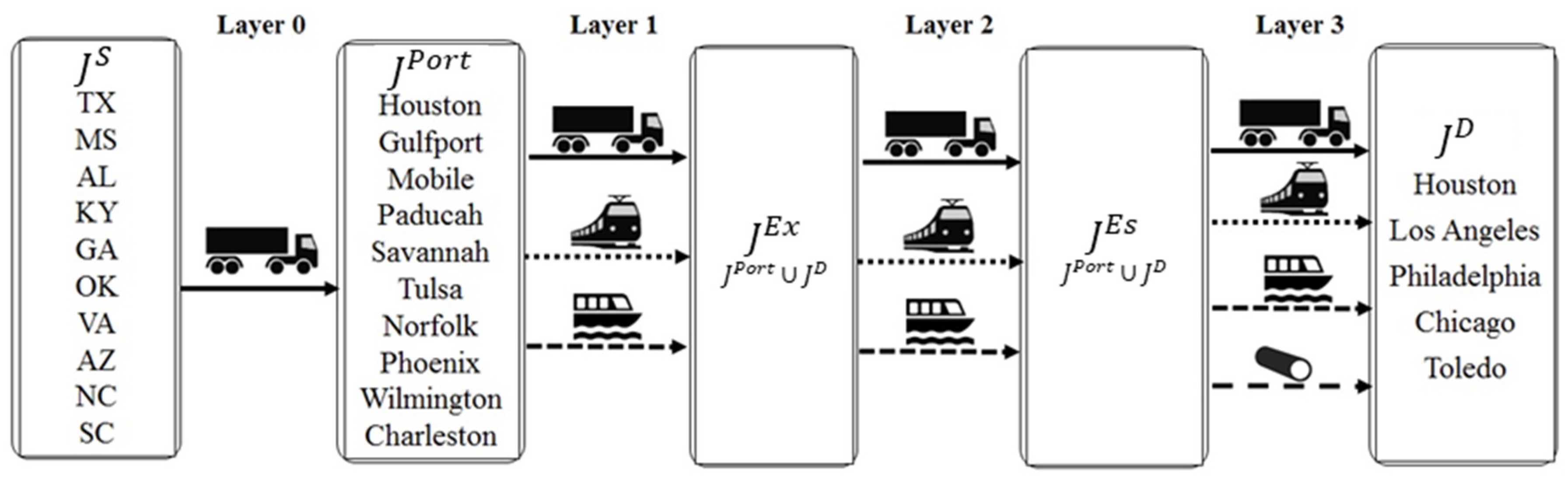
4.2. United States of America

The second case examined is that of the algal biomass to biodiesel supply chain for the contiguous United States. As with the case of the state of Oklahoma, two criteria, historical weather data and availability of marginal farmland, were used to determine the potential algae biomass supply locations, and the utilized algae species is once again I. galbana. Average monthly temperatures from 1971 to 2000 were examined using the National Oceanic and Atmospheric Administration (NOAA) average mean temperature index by month [33], and the states with historical average temperatures below freezing were excluded from consideration as potential algae suppliers. This reduced the number of supply locations to 19. In addition, the amount of marginal farmland available is calculated in much the same way as was done with the Oklahoma case, with state values used instead of individual counties. The remaining states were ranked based on the availability of marginal farmland and the top 50% were taken as potential supply locations, given in the first column of

Table 3. Supply locations for the United States case of the algal biomass to biodiesel problem.

Supply Locations	Marginal Farmland Availability	Farm Real Estate, ($/m2)	Water Cost ($/1000 Gallons)	Supply Port Cities
$\left({\mathit{J}}^{\mathit{S}}\right)$	(km2)			$\left({\mathit{J}}^{\mathit{P}\mathit{o}\mathit{r}\mathit{t}}\right)$
Texas	44,900	0.447	0.02867	Houston
Mississippi	14,500	0.529	0.01311	Gulfport
Alabama	14,200	0.494	0.01605	Mobile
Kentucky	13,100	0.815	0.00602	Paducah
Georgia	10,900	0.890	0.01343	Savannah
Oklahoma	10,800	0.393	0.01968	Tulsa
Virginia	8910	1.124	0.01442	Norfolk
Arizona	8820	0.939	0.04774	Phoenix
North Carolina	8520	1.124	0.01057	Wilmington
South Carolina	8500	0.704	0.01142	Charleston

.

Table 3 also shows the state’s average farm real estate values as determined by the USDA NASS [27]. Water cost was taken as the average energy expenses for irrigation water in each state, again as determined by the USDA NASS [27], assuming that the average acre of cropland requires 10,000 m³ of water per year [31]. Each supply location has a port city, chosen because of its connectivity to truck, rail, pipeline, and in most cases, barge transportation modes. It was assumed that all algae biomass left each supply state through this port city. Because of this, the Google maps [34] distance between the geographic center of the state and the port city was used to represent the average distance between farms in the state and the port. Weather data (minimum and maximum temperatures, relative humidity, and wind velocity) was calculated using the Mathematica WeatherData database [35].

It was assumed that all deliveries would be made to the port cities in the demand location. Both supply port cities and demand port cities were considered as possible locations for extraction and transesterification. Table 3,

Table 4. Extraction and transesterification locations for the United States case of the algal biomass to biodiesel problem.

$\mathbf{Extraction}\mathbf{Locations}\left({\mathit{J}}^{\mathit{E}\mathit{x}}\right)$	$\mathbf{Transesterification}\mathbf{Locations}\left({\mathit{J}}^{\mathit{E}\mathit{s}}\right)$
Houston	Houston
Gulfport	Gulfport
Mobile	Mobile
Paducah	Paducah
Savannah	Savannah
Tulsa	Tulsa
Norfolk	Norfolk
Phoenix	Phoenix
Wilmington	Wilmington
Charleston	Charleston
Los Angeles	Los Angeles
Philadelphia	Philadelphia
Chicago	Chicago
Toledo	Toledo

and

Table 5. Demand locations for the United States case of the algal biomass to biodiesel problem.

$\mathbf{Demand}\mathbf{Locations}\left({\mathit{J}}^{\mathit{D}}\right)$	$\mathbf{Demand}\mathbf{Port}\mathbf{Cities}\left({\mathit{J}}^{\mathit{D},\mathit{P}\mathit{o}\mathit{r}\mathit{t}}\right)$	Demand (kt yr−1)
Texas	Houston	24,038
California	Los Angeles	12,570
Pennsylvania	Philadelphia	7999
Illinois	Chicago	6518
Ohio	Toledo	6617

list all the supply locations, port locations, extraction locations, transesterification locations, and demand locations. Those states with the highest 10% of diesel sales were taken as demand locations [36] and are shown in the first column of Table 5. Figure 10 shows geographically the supply states (outlined in green) and demand states (filled with red).

While the Oklahoma case only considered transportation by truck, the case of the United States considers rail, barge, and pipeline transport. Therefore, road distances were taken as the shortest route found using Google maps between locations [34]. Rail distances were measured using the U.S. Department of Transportation’s Bureau of Transportation Statistics National Transportation Atlas Database of Railway Networks [37], with the nearest railway to the shortest Google maps road route taken as the shortest rail route. Barge distances were calculated as distances between ports [38]. Pipeline distances were taken using the U.S. Energy Information Administration (EIA) petroleum product pipeline database, with the nearest pipeline to the shortest Google maps road route taken as the shortest pipeline route [39]. All the distances associated with trucks, rails, barges, and pipelines between supply, port, extraction, transesterification, and demand locations are given Appendix A via

Table A2. Road distances between Supply and Port locations (km).

Supply-Port	Distance (km)
Texas-Houston	547.178
Mississippi-Gulfport	313.823
Alabama-Mobile	313.823
Kentucky-Paducah	386.243
Georgia-Savannah	225.309
Oklahoma-Tulsa	307.385
Virginia-Norfolk	373.369
Arizona-Phoenix	131.806
North Carolina-Wilmington	247.839
South Carolina-Charleston	146.451

,

Table A3. Road distances between Port and Extraction locations (km).

	Gulfport	Mobile	Paducah	Savannah	Tulsa	Norfolk	Phoenix
Houston	649	753	1213	1619	798	2226	1893
Gulfport	0	120	851	987	1109	1592	2536
Mobile	120	0	805	869	1152	1476	2643
Paducah	851	805	0	1012	768	1350	2480
Savannah	987	869	1012	0	1659	772	3368
Tulsa	1109	1152	768	1659	0	2103	1714
Norfolk	1592	1476	1350	772	2103	0	3767
Phoenix	2536	2643	2480	3368	1714	3767	0
Wilmington	1302	1186	1249	484	1926	444	3637
Charleston	1128	1012	1101	171	1753	707	3463
	Wilmington	Charleston	Houston	Los Angeles	Philadelphia	Chicago	Toledo
Houston	1936	1762	0	2491	2486	1743	1999
Gulfport	1302	1128	649	3135	1902	1445	1556
Mobile	1186	1012	753	3241	1786	1426	1481
Paducah	1249	1101	1213	3072	1432	600	856
Savannah	484	171	1619	3898	1156	1535	1323
Tulsa	1926	1753	798	2308	2058	1110	1389
Norfolk	444	707	2226	4360	446	1423	1056
Phoenix	3637	3463	1893	599	3767	2821	3098
Wilmington	0	280	1936	4168	824	1521	1221
Charleston	280	0	1762	3994	1086	1466	1254

,

Table A4. Road distances between Extraction and Transesterification locations (km).

	Gulfport	Mobile	Paducah	Savannah	Tulsa	Norfolk	Phoenix
Gulfport	0	120	851	987	1109	1592	2536
Mobile	120	0	805	869	1152	1476	2643
Paducah	851	805	0	1012	768	1350	2480
Savannah	987	869	1012	0	1659	772	3368
Tulsa	1109	1152	768	1659	0	2103	1714
Norfolk	1592	1476	1350	772	2103	0	3767
Phoenix	2536	2643	2480	3368	1714	3767	0
Wilmington	1302	1186	1249	484	1926	444	3637
Charleston	1128	1012	1101	171	1753	707	3463
Houston	649	753	1213	1619	798	2226	1893
Los Angeles	3135	3241	3072	3898	2308	4360	599
Philadelphia	1902	1786	1432	1156	2058	446	3767
Chicago	1445	1426	600	1535	1110	1423	2821
Toledo	1556	1481	856	1323	1389	1056	3098
	Wilmington	Charleston	Houston	Los Angeles	Philadelphia	Chicago	Toledo
Gulfport	1302	1128	649	3135	1902	1445	1556
Mobile	1186	1012	753	3241	1786	1426	1481
Paducah	1249	1101	1213	3072	1432	600	856
Savannah	484	171	1619	3898	1156	1535	1323
Tulsa	1926	1753	798	2308	2058	1110	1389
Norfolk	444	707	2226	4360	446	1423	1056
Phoenix	3637	3463	1893	599	3767	2821	3098
Wilmington	0	280	1936	4168	824	1521	1221
Charleston	280	0	1762	3994	1086	1466	1254
Houston	1936	1762	0	2491	2486	1743	1999
Los Angeles	4168	3994	2491	0	4363	3244	3613
Philadelphia	824	1086	2486	4363	0	1221	853
Chicago	1521	1466	1743	3244	1221	0	394
Toledo	1221	1254	1999	3613	853	394	0

,

Table A5. Road distances between Transesterification and Demand locations (km).

	Houston	Los Angeles	Philadelphia	Chicago	Toledo
Gulfport	649	3135	1902	1445	1556
Mobile	753	3241	1786	1426	1481
Paducah	1213	3072	1432	600	856
Savannah	1619	3898	1156	1535	1323
Tulsa	798	2308	2058	1110	1389
Norfolk	2226	4360	446	1423	1056
Phoenix	1893	599	3767	2821	3098
Wilmington	1936	4168	824	1521	1221
Charleston	1762	3994	1086	1466	1254
Houston	0	2491	2486	1743	1999
Los Angeles	2491	0	4363	3244	3613
Philadelphia	2486	4363	0	1221	853
Chicago	1743	3244	1221	0	394
Toledo	1999	3613	853	394	0

,

Table A6. Rail distances between Port and Extraction locations (km).

	Gulfport	Mobile	Paducah	Savannah	Tulsa	Norfolk	Phoenix
Houston	681	798	1291	1725	845	2348	1952
Gulfport	0	117	840	1044	1104	1667	2633
Mobile	117	0	782	927	1133	1550	2750
Paducah	840	782	0	1078	851	1366	2815
Savannah	1044	927	1078	0	1730	847	3677
Tulsa	1104	1133	851	1730	0	2160	1976
Norfolk	1667	1550	1366	847	2160	0	4146
Phoenix	2633	2750	2815	3677	1976	4146	0
Wilmington	1362	1244	1289	465	2150	381	3922
Charleston	1135	1017	1044	174	1819	673	3661
	Wilmington	Charleston	Houston	Los Angeles	Philadelphia	Chicago	Toledo
Houston	2042	1815	0	2593	2607	1732	1983
Gulfport	1362	1135	681	3273	1926	1605	1659
Mobile	1244	1017	798	3391	1809	1487	1542
Paducah	1289	1044	1291	3391	1498	558	805
Savannah	465	174	1725	4318	1188	1637	1447
Tulsa	2150	1819	845	2617	1498	1107	1382
Norfolk	381	673	798	3391	1809	1487	1542
Phoenix	3922	3661	1952	641	4081	3075	3352
Wilmington	0	291	2042	4562	2042	1524	1215
Charleston	291	0	1815	4302	1815	1545	1284

,

Table A7. Rail distances between Extraction and Transesterification locations (km).

	Gulfport	Mobile	Paducah	Savannah	Tulsa	Norfolk	Phoenix
Gulfport	0	117	840	1044	1104	1667	2633
Mobile	117	0	782	927	1133	1550	2750
Paducah	840	782	0	1078	851	1366	2815
Savannah	1044	927	1078	0	1730	847	3677
Tulsa	1104	1133	851	1730	0	2160	1976
Norfolk	1667	1550	1366	847	2160	0	4146
Phoenix	2633	2750	2815	3677	1976	4146	0
Wilmington	1362	1244	1289	465	2150	381	3922
Charleston	1135	1017	1044	174	1819	673	3661
Houston	681	798	1291	1725	845	798	1952
Los Angeles	3273	3391	3391	4318	2617	3391	641
Philadelphia	1926	1809	1498	1188	1498	1809	4081
Chicago	1605	1487	558	1637	1107	1487	3075
Toledo	1659	1542	805	1447	1382	1542	3352
	Wilmington	Charleston	Houston	Los Angeles	Philadelphia	Chicago	Toledo
Gulfport	1362	1135	681	3273	1926	1605	1659
Mobile	1244	1017	798	3391	1809	1487	1542
Paducah	1289	1044	1291	3391	1498	558	805
Savannah	465	174	1725	4318	1188	1637	1447
Tulsa	2150	1819	845	2617	1498	1107	1382
Norfolk	381	673	798	3391	1809	1487	1542
Phoenix	3922	3661	1952	641	4081	3075	3352
Wilmington	0	291	2042	4562	2042	1524	1215
Charleston	291	0	1815	4302	1815	1545	1284
Houston	2042	1815	0	2593	2607	1732	1983
Los Angeles	4562	4302	2593	0	4260	3219	3648
Philadelphia	2042	1815	2607	4260	0	1165	808
Chicago	1524	1545	1732	3219	1165	0	357
Toledo	1215	1284	1983	3648	808	357	0

,

Table A8. Rail distances between Transesterification and Demand locations (km).

	Houston	Los Angeles	Philadelphia	Chicago	Toledo
Gulfport	681	3273	1926	1605	1659
Mobile	798	3391	1809	1487	1542
Paducah	1291	3391	1498	558	805
Savannah	1725	4318	1188	1637	1447
Tulsa	845	2617	1498	1107	1382
Norfolk	798	3391	1809	1487	1542
Phoenix	1952	641	4081	3075	3352
Wilmington	2042	4562	2042	1524	1215
Charleston	1815	4302	1815	1545	1284
Houston	0	2593	2607	1732	1983
Los Angeles	2593	0	4260	3219	3648
Philadelphia	2607	4260	0	1165	808
Chicago	1732	3219	1165	0	357
Toledo	1983	3648	808	357	0

,

Table A9. Barge distances between Port and Extraction locations (km).

	Gulfport	Mobile	Paducah	Savannah	Tulsa	Norfolk
Houston	772	906	2260	2769	2330	3700
Gulfport	0	134	1487	1996	1802	2927
Mobile	134	0	1353	1862	1936	2794
Paducah	1487	1353	0	3574	1362	4506
Savannah	1996	1862	3574	0	3645	932
Tulsa	1802	1936	1362	3645	0	4577
Norfolk	2927	2794	4506	932	4577	0
Wilmington	2416	2282	3994	420	4065	512
Charleston	2184	2050	3763	188	3833	744
	Wilmington	Charleston	Houston	Philadelphia	Chicago	Toledo
Houston	3188	2956	0	4030	3072	4179
Gulfport	2416	2184	772	3257	2544	3652
Mobile	2282	2050	906	3124	2678	3785
Paducah	3994	3763	2260	5768	1497	2604
Savannah	420	188	2768	1262	4387	5494
Tulsa	4065	3833	2330	4907	2174	3281
Norfolk	512	744	3700	330	5319	6426
Wilmington	0	232	3188	842	4807	5914
Charleston	232	0	2956	1073	4575	5683

,

Table A10. Barge distances between Extraction and Transesterification locations (km).

	Gulfport	Mobile	Paducah	Savannah	Tulsa	Norfolk
Gulfport	0	134	1487	1996	1802	2927
Mobile	134	0	1353	1862	1936	2794
Paducah	1487	1353	0	3574	1362	4506
Savannah	1996	1862	3574	0	3645	932
Tulsa	1802	1936	1362	3645	0	4577
Norfolk	2927	2794	4506	932	4577	0
Wilmington	2416	2282	3994	420	4065	512
Charleston	2184	2050	3763	188	3833	744
Houston	772	906	2260	2768	2330	3700
Philadelphia	3257	3124	5768	1262	4907	330
Chicago	2544	2678	1497	4387	2174	5319
Toledo	3652	3785	2604	5494	3281	6426
	Wilmington	Charleston	Houston	Philadelphia	Chicago	Toledo
Gulfport	2416	2184	772	3257	2544	3652
Mobile	2282	2050	906	3124	2678	3785
Paducah	3994	3763	2260	5768	1497	2604
Savannah	420	188	2768	1262	4387	5494
Tulsa	4065	3833	2330	4907	2174	3281
Norfolk	512	744	3700	330	5319	6426
Wilmington	0	232	3188	842	4807	5914
Charleston	232	0	2956	1073	4575	5683
Houston	3188	2956	0	4030	3072	4179
Philadelphia	842	1073	4030	0	5649	6756
Chicago	4807	4575	3072	5649	0	1107
Toledo	5914	5683	4179	6756	1107	0

,

Table A11. Barge distances between Transesterification and Demand locations (km).

	Houston	Philadelphia	Chicago	Toledo
Gulfport	772	3257	2544	3652
Mobile	906	3124	2678	3785
Paducah	2260	5768	1497	2604
Savannah	2768	1262	4387	5494
Tulsa	2330	4907	2174	3281
Norfolk	3700	330	5319	6426
Wilmington	3188	842	4807	5914
Charleston	2956	1073	4575	5683
Houston	0	4030	3072	4179
Philadelphia	4030	0	5649	6756
Chicago	3072	5649	0	1107
Toledo	4179	6756	1107	0

and

Table A12. Pipeline distances between Transesterification and Demand locations (km).

	Houston	Los Angeles	Philadelphia	Chicago	Toledo
Gulfport	790	3306	1844	2187	2393
Mobile	835	3351	1907	2189	2406
Paducah	1157	3421	1873	568	768
Savannah	1506	4022	1539	2694	2338
Tulsa	726	2791	2055	993	1308
Norfolk	2020	2828	583	1738	1382
Phoenix	1878	637	3766	2763	3071
Wilmington	1944	4460	924	2079	1724
Charleston	1653	4168	1247	2403	2047
Houston	0	2515	2245	1584	1838
Los Angeles	2515	0	4403	3401	3708
Philadelphia	2245	4403	0	1156	800
Chicago	1584	3401	1156	0	415
Toledo	1838	3708	800	415	0

. The entire system of transportation options is shown in Figure 11. It should be noted that pipeline is only taken as a transportation route between the transesterification and demand locations, as the network of pipelines examined is that used for transportation of products, rather than crude oil. To investigate the impact of spacial disconnect of the major shipping hubs from land that would be used to grow the algae, Layer 0 is introduced for this implementation of the model. The introduction of layer 0 necessitates the introduction of variables $N_{Truck,j^S,j^{Port}}^0,$ $o_{Truck,j^S,j^{Port}}^0$, and $O_{j^{Port}}^{Port}$ with the associated constraints to account for the number of trucks shipping product from supply location $j^S\in J^S$ to port location $j^{Port}\in J^{Port}$, the amount of product shipped from supply location $j^S\in J^S$ to port location $j^{Port}\in J^{Port}$, and the total amount of product at port location $j^{Port}\in J^{Port}$, respectively.

For Layer 0, to transport dry algae biomass, only trucks were considered; for layers 1 and 2, trucks, rails, barges were considered; and for layer 3, pipelines were added to carry the biodiesel along with the other modes. The capacities, ${\mathsf{\Xi }}_z$, for $z\in \left\{\mathrm{truck},\mathrm{rail},\mathrm{barge}\right\}$ are 30 m³, 113.56 m³, and 1192 m³, respectively. Here, the capacity of the pipeline is equivalent to the number of pipelines, i.e., it is equal to one. It should be noted that there is no barge transportation to and from Phoenix and Los Angeles. Therefore, additional constraints must be added to the variables associated with barge transportation for these cities to constrain products shipped to and from these cities using barges to zero, see Equations (38)–(43).

$$o_{Barge,j^{Port},j^{Ex}}^1=0 kt \forall j^{Port}\in \left\{Phoenix,Los Angeles\right\},\forall j^{Ex}\in J^{Ex},$$

(38)

$$o_{Barge,j^{Port},j^{Ex}}^1=0 kt \forall j^{Port}\in J^{Port},\forall j^{Ex}\in \left\{Phoenix,Los Angeles\right\},$$

(39)

$$o_{Barge,j^{Ex},j^{Es}}^2=0 kt \forall j^{Ex}\in \left\{Phoenix,Los Angeles\right\}, \forall j^{Es}\in J^{Es},$$

(40)

$$o_{Barge,j^{Ex},j^{Es}}^2=0 kt \forall j^{Ex}\in J^{Ex},\forall j^{Es}\in \left\{Phoenix,Los Angeles\right\},$$

(41)

$$o_{Barge,j^{Es},j^D}^3=0 kt \forall j^{Es}\in \left\{Phoenix,Los Angeles\right\}, \forall j^D\in J^D,$$

(42)

$$o_{Barge,j^{Es},j^D}^3=0 kt \forall j^{Es}\in j^{Es}, \forall j^D\in \left\{Los Angeles\right\}.$$

(43)

5. Solution Approach

The resulting mixed-integer nonlinear program (MINLP) is a large scale non-convex problem, and it is implemented in GAMS Version 24.7.1 using an Intel^® Xeon^® E5-2650 v3, 2.30 GHz processor running Windows 10. The only integer variable is the number of ponds, $N_j^{Pond}$, at each supply locations $j\in J^S$. This MINLP is unable to be solved using global MINLP solvers: ANTIGONE version 1.1, and BARON version 18.11.15. We also attempted to solve this problem using a local MINLP solver without success. However, relaxing the integrality constraints yields a non-convex nonlinear programming (NLP) formulation, which will be referred to as the relaxed-MINLP, that is solvable. The optimum solution of the relaxed-MINLP provides a lower bound for the original MINLP. Unfortunately, global solvers (BARON version 18.11.15 and ANTIGONE version 1.1) and the local solver (DICOPT) were not able to solve the problem to optimality. Therefore, the relaxed-MINLP is solved using CONOPT 3 version 3.17A with a multi-start approach. Although this approach does not guarantee that the optimum solution of the relaxed-MINLP is obtained, it allows to generate the reasonable values of $A_j^{Pond}$, $f_{j,y}^{DA}$, $V_j^{Ind}$, $P{P}_{j,d,t}$, and $P{W}_{j,d,t}$ that can be fixed in the original MINLP model.

The nonlinear equations of the model are Equations (5)–(7), (10), (11), (30), (32) and (34). The incorporation of the pond model also introduces non-linearities in the model through the operational values of the pond, i.e., average fluid velocity in the raceway pond or temperature of the pond. If the values of $A_j^{Pond}$, $f_{j,y}^{DA}$, $V_j^{Ind}$, $P{P}_{j,d,t}$, and $P{W}_{j,d,t}$ are fixed to the solution obtained from the relaxed-MINLP, the resulting mathematical program is a mixed-integer linear program (MILP). The solution of this MILP is a feasible solution to the original MINLP, hence an upper bound for the original MINLP. The MILP is solved using CPLEX version 12.6.3.0. We report this feasible solution in this paper. A relative gap is calculated using the MILP and relaxed-MINLP solutions.

6. Results and Discussion

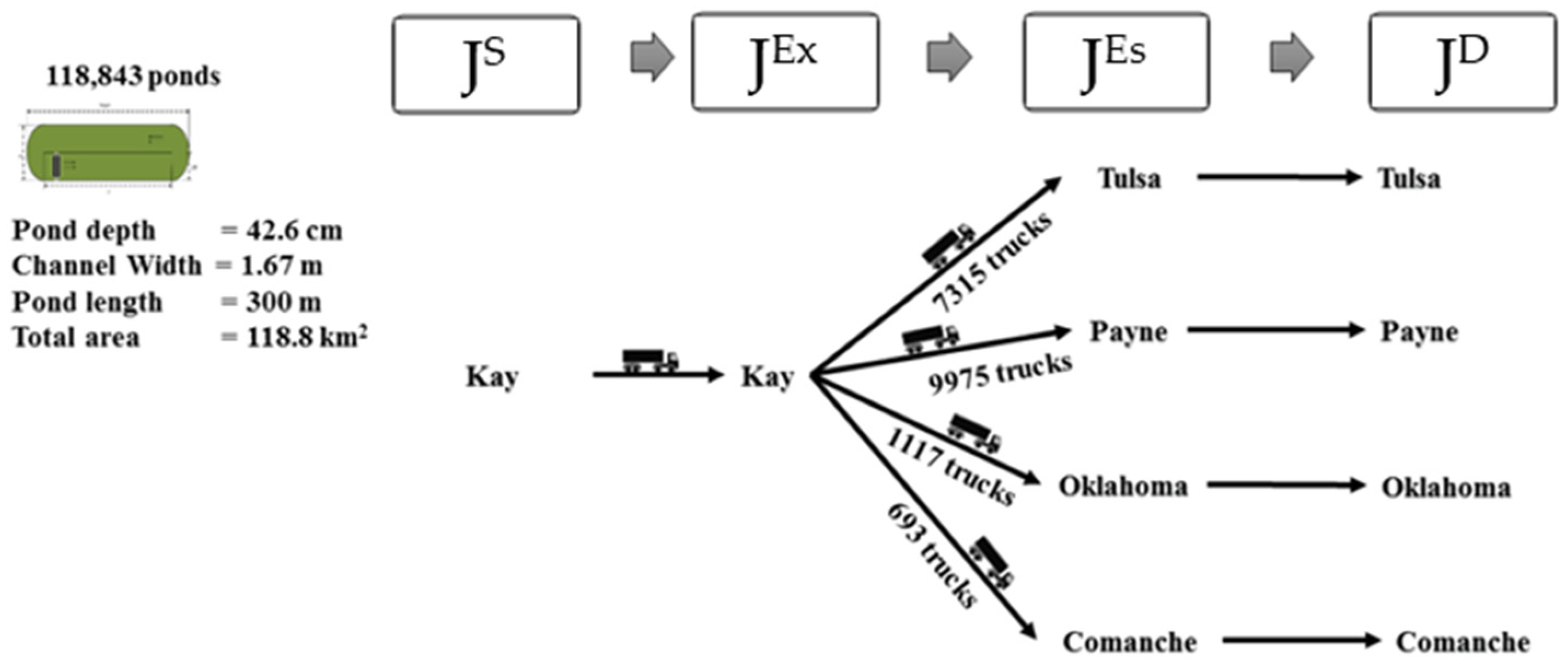
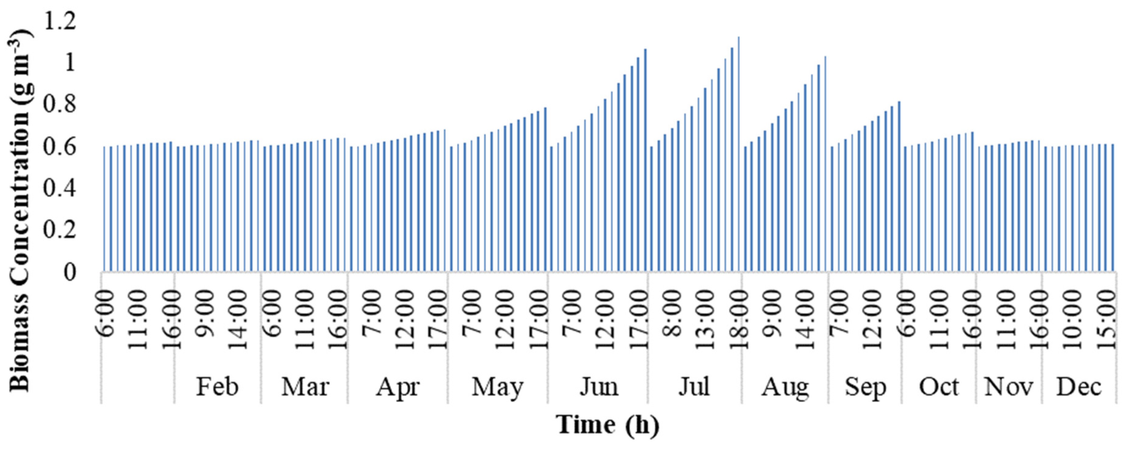
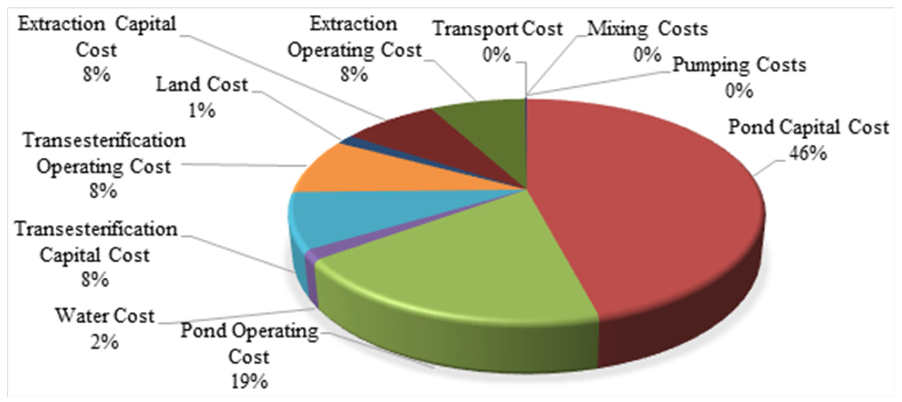
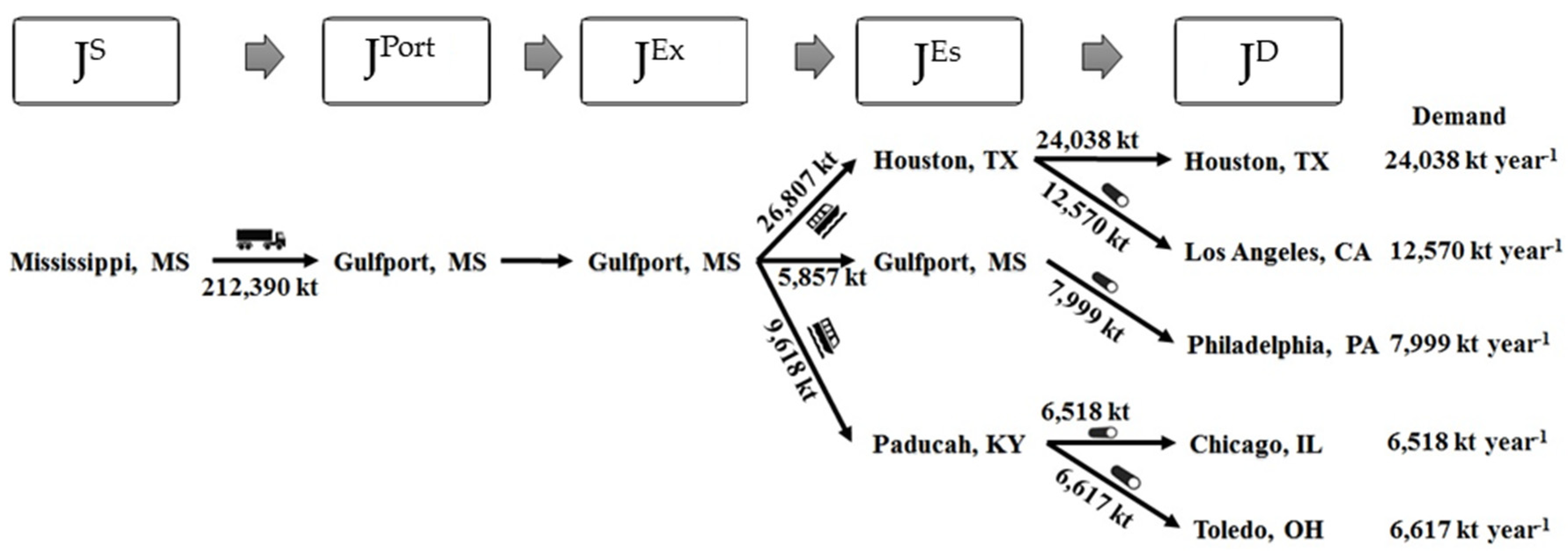
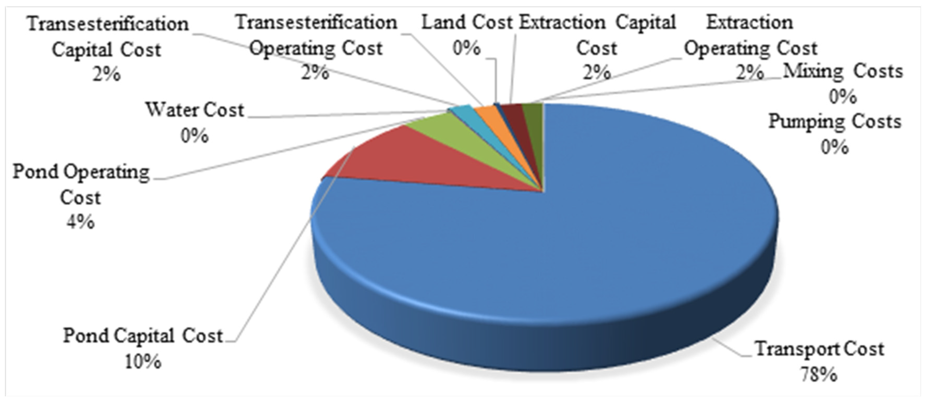
6.1. Oklahoma Case Study

Table 6. Comparison of the solutions from relaxed-mixed-integer nonlinear program (MINLP) and mixed-integer linear programming (MILP) solvers: CONOPT 3 version 3.17A and CPLEX version 12.6.3.0 for the case of Oklahoma.

	Relaxed-MINLP	MILP
Total Cost ($)	9.921 billion	9.921 billion
Pond Capital Cost ($)	1.562 billion	1.562 billion
Pond Operating Cost ($)	650.7 million	650.7 million
Transport Cost ($)	705.7 thousand	705.7 thousand
Number of Ponds	Garfield = 0.426	Kay = 118843
	Grant = 0.426
	Jackson = 0.426
	Kay = 118842.27
	Tillman = 0.426
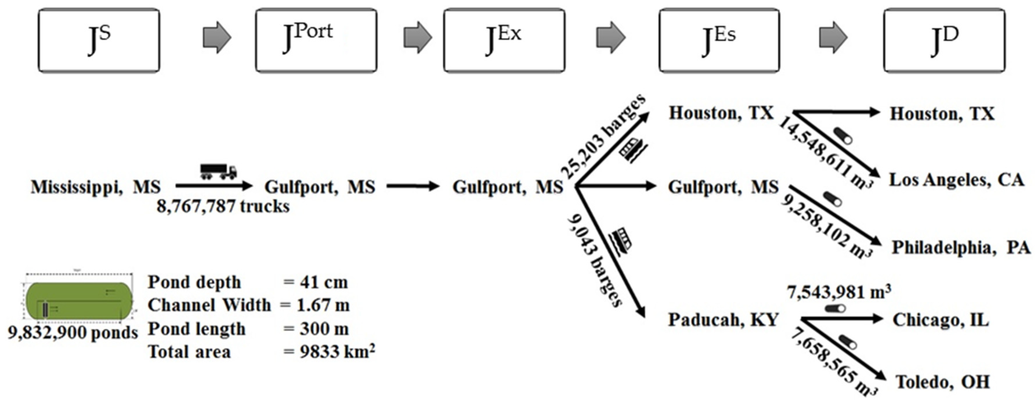
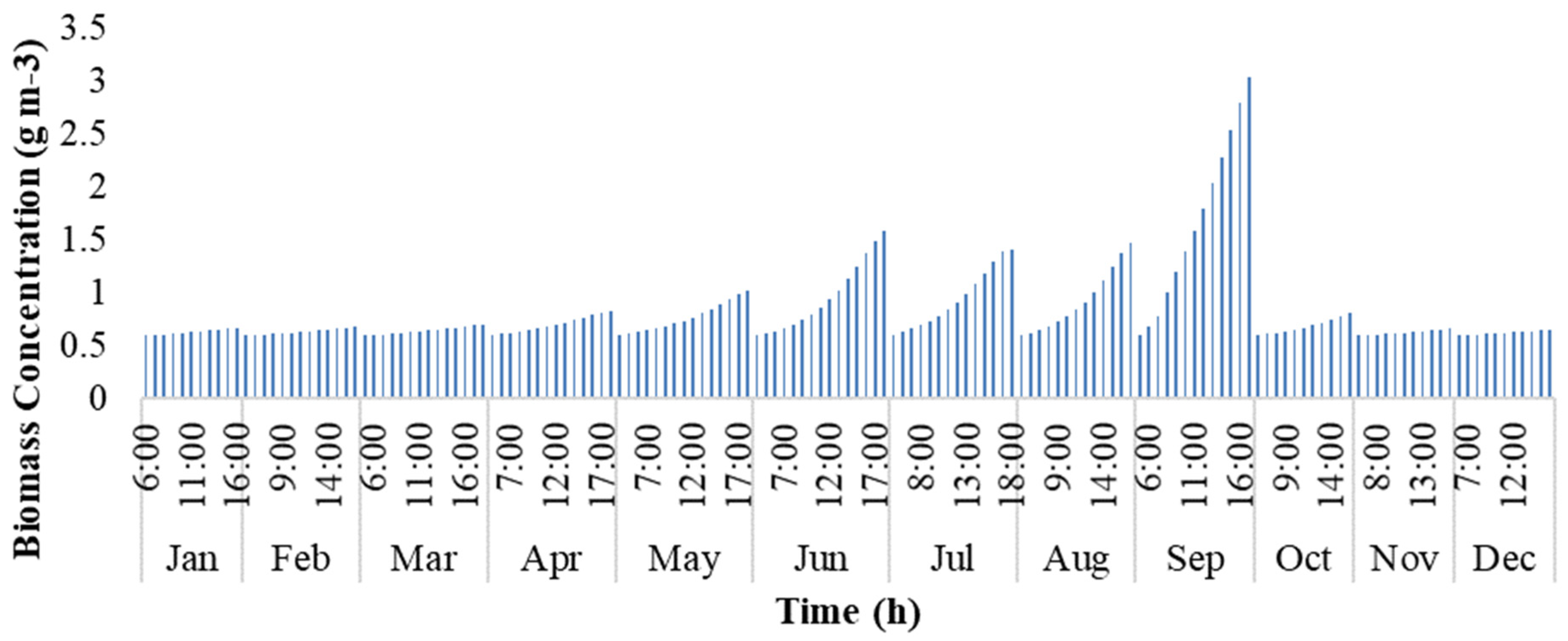
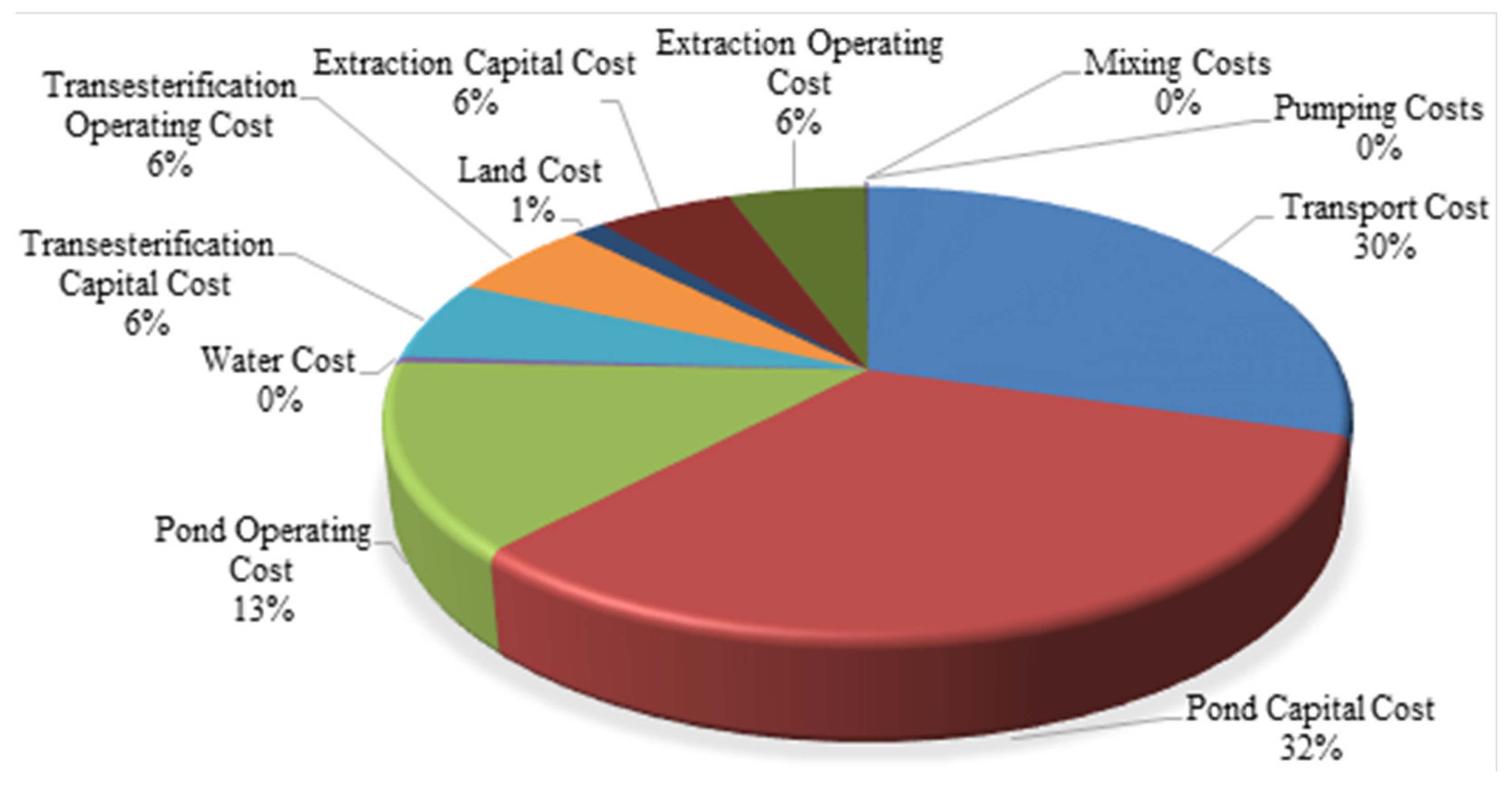
	Woods = 0.426

shows the objective function values of the relaxed-MINLP problem and the MILP problem at the first iteration. The main difference between the relaxed-MINLP and MILP objective function values stem from the number of ponds, $N_j^{Pond}$, required at each location $j\in J^S$, which is a fractional value for the relaxed-MINLP solution. Hence, the capital, $C{C}^S$, and operating costs, $CO$, associated with raceway ponds, and the transportation cost, $TrC$, change slightly to account for the small amount of algal biomass produced at locations with fractional ponds.

Table 7. Computational and model statistics for the Oklahoma case.

	Total Variables	Continuous Variables	Integer Variables	Constraints	Solution Time (h:m:s)
MINLP	25,691	25,685	6	29,112	N/A
Relaxed-MINLP	25,691	25,691	N/A	29,112	00:28:52.42
MILP	466	460	6	302	00:00:00.11

shows the computational statistics for the Oklahoma case, including the model size and solution time. The solution time for the MINLP shows ‘N/A’ as the solvers used were unable to find a solution.

The resulting supply chain topology is summarized in Figure 12, which shows the supply, extraction, and transesterification locations selected to meet the demand. This figure also shows the number of trucks needed to transport the algae oil from the extraction to the transesterification sites, as well as providing the raceway pond dimensions, such as pond depth, channel width, and pond length; number of such ponds required to meet the demand; and area of algae cultivation farmland necessary to meet the demand. It can be observed that more than 72% of the available marginal farmland of Kay County must be used for the cultivation of algae biomass to meet the biodiesel demand. When the total cost is minimized, it was found that the demand in all of the state of Oklahoma demand regions can be met with 118,843 ponds in Kay County. The algal biomass produced in Kay County is then extracted in Kay County. Next, the algae oil is shipped for transesterification at each of the demand counties in the amount needed to produce biodiesel to meet the demand in that particular county. A total of 19,096 trucks are needed to transport the algae oil. Additionally, the total fuel consumption of the trucks needed to transport algal oil was calculated and is presented in

Table 8. Fuel consumption and demand for the Oklahoma case.

	Flat-Rate Fuel Consumption (gal)	Weight-Based Fuel Consumption (gal)
Transportation Fuel Requirements	141,594	247,088
Fuel Demand	213,380,041	213,480,041
% of fuel needed of demand	0.066%	0.116%

. Two different means were used to calculate the fuel consumption: a flat rate of fuel consumption measured in gal/km traveled [40] and a weight-based fuel consumption accounting for the total weight of the truck measured in gal/(100-t km) [41]. The total fuel consumption is less than a percent of the fuel demand of Oklahoma, showing little to no impact on the total demand and profitability of the supply chain. This is due to the relatively short distances traveled and the small number of trucks needed for the transportation of the fuel or its precursors.

Figure 13 shows how biomass concentration changes during the course of the day from sunrise to sunset. It can be observed that, in one representative day of a month, biomass concentration gradually increases from sunrise until it reaches sunset. This is because of the accumulation of biomass with the time of the day or until harvest. The biomass concentration and production are rapid in the summer months of June, July, August, and September. However, July was found to be the favorable month for the species I. galbana because optimal conditions for growth exist during that month for the Kay County location.

Figure 14 shows the breakdown of the overall cost. The supply chain network has a total cost of $9.921 billion over ten years, at a per U.S. gallon cost of $7.07 (corresponding to $1.87 per liter). Of the cost, 46% is due to the capital costs associated with raceway ponds, and 19% is due to the raceway pond operating cost. The capital and operating costs for extraction and transesterification each make up 8% of the cost. The cost of transportation is relatively small compared to the overall supply chain cost (and compared to the transportation costs of the United States case) due to the relatively short distances over which the algae oil is transported.

6.2. United States

Table 9. Comparison of the solution from relaxed-MINLP and MILP solvers: CONOPT 3 version 3.17 A and CPLEX version 12.6.3.0 for the U.S. case.

	Relaxed-MINLP	MILP
Total Cost ($)	6.625 trillion	6.625 trillion
Pond Capital Cost ($)	129.244 billion	129.244 billion
Pond Operating Cost ($)	53.835 billon	53.835 billon
Transport Cost ($)	965.488 billion	965.488 billion
Number of Ponds	Houston = 0.01079	Gulfport = 9832912
	Gulfport = 9832911.165
	Mobile = 0.01079
	Paducah = 0.01079
	Savannah = 38.939
	Tulsa = 0.01079
	Norfolk = 0.01079
	Phoenix = 0.01079
	Wilmington = 0.01079
	Charleston = 0.01079

shows the objective function values of the relaxed-MINLP problem and the MILP problem at the first iteration. The relative optimality gap is zero, and hence no iterations were required. It should be noted that this solution is a local optimum for this problem. The main difference between the relaxed-MINLP and MILP objective function values stem from the number of ponds, $N_j^{Pond}$, required at each location $j\in J^S$, which is a fractional value for the relaxed-MINLP solution. Hence, the capital, $C{C}^S$, and operating costs, $O{C}^S$, associated with raceway ponds, and the transportation cost, $TrC$, change slightly to account for the small amount of algal biomass produced at locations with fractional ponds.

Table 10. Computational and model statistics for the U.S. case.

	Total Variables	Continuous Variables	Integer Variables	Constraints	Solution Time (h:m:s)
MINLP	40,238	40,228	10	46,496	N/A
Relaxed-MINLP	40,238	40,238	N/A	46,496	01:46:22.72
MILP	2706	2696	10	2975	00:00:00.09

shows the computational statistics for the USA case, including the model size and the solution time. The solution time for the MINLP shows ‘N/A’ as the solvers used were unable to find a solution.

The resulting supply chain topology is summarized in Figure 15, which shows the supply, port, extraction, and transesterification locations selected to meet the demand and the method of transportation selected for distributing the products from one location to another. The figure shows the number of trucks, barges, and pipelines required to carry the products. Notice that there are no transport vehicles between the same locations. The figure also provides the single raceway pond dimensions, such as pond depth, channel width, pond length, number of such ponds required to meet the demand, and the area they occupy. It was found that in order to meet the biodiesel demand, the state of Mississippi uses more than 65% of the available marginal farmland for the cultivation of algae biomass. The total fuel consumption of the supply chain was once again calculated and is presented in

Table 11. Fuel consumption and demand for the U.S. case.

	Flat-Rate Fuel Consumption (gal)	Weight-Based Fuel Consumption (gal)
Transportation Fuel Requirements	3,005,783,939	1,356,895,409
Fuel Demand	17,654,883,824	17,654,883,824
% of fuel needed of demand	17.025%	7.686%

. The first column shows the fuel consumption using a flat-rate calculation [40,42], and the second column shows the fuel consumption on a weight-based calculation [41]. The relatively large range of fuel consumption is due to the difference in calculating the fuel consumption of the barges. When using a weight-based calculation, barges are projected to consume two to three times less fuel than when using a flat-rate calculation. The inverse is true for fuel consumption of trucks. Nevertheless, both means of calculations reveal that a sizeable amount of fuel is used for transportation within the supply chain. Although the need for fuel to transport the products of this supply chain is not close to the overall demand for diesel, the results suggest that it may impose an economic burden on this supply chain.

Inside the pond, there are dynamic changes occurring in biomass concentration. Figure 16 shows how biomass concentration changes during the course of the day from sunrise to sunset. It can be observed that in one representative day of a month, biomass concentration gradually increases from sunrise to sunset. However, September was found to be the favorable month for the species I. galbana because optimal conditions for growth exist during that month and Mississippi location.

Figure 17 shows the amounts of products transported between different layers. The solution reveals that among the various supply locations considered (Texas, Mississippi, Alabama, Kentucky, Georgia, Oklahoma, Virginia, Arizona, North Carolina, and South Carolina), Mississippi was selected for algae cultivation based on the model parameters, such as availability of farmland area and weather data. This location has favorable conditions for the cultivation of algae biomass, together with the high availability of marginal farmland compared to the other states.

As per our model assumptions, dry algae biomass from each supply location is transported to their respective port cities via trucks. From the available ten supply–port combinations (Texas–Houston, Mississippi–Gulfport, Alabama–Mobile, Kentucky–Paducah, Georgia–Savannah, Oklahoma–Tulsa, Virginia–Norfolk, Arizona–Phoenix, North Carolina–Wilmington, and South Carolina–Charleston), since algae cultivation occurs only in Mississippi, algae biomass was shipped to its respective port city of Gulfport ($o_{\mathrm{Truck},\mathrm{Mississippi},\mathrm{Gulfport}}^1$) = 212,390 kt) via trucks.

The solution suggests that among the choices of all the port and demand locations, algae oil is extracted at the port city where biomass was shipped. This route was selected because the transportation costs between layers with the same locations are zero. Part of the extracted algae oil at the Gulfport, MS, USA, is processed to biodiesel at its current location (5857 kt), and the remainder is shipped to Houston, TX, USA ($o_{\mathrm{Barge},\mathrm{Gulfport},\mathrm{Houston}}^2$ = 26,807 kt), and Paducah, KY, USA ($o_{\mathrm{Barge},\mathrm{Gulfport},\mathrm{Paducah}}^2$ = 9618 kt), via barges for further processing into biodiesel. Upon further investigation on the choice of barges over the other methods of transportation for transporting algae oil, it was found that although the cost of shipping through barges was expensive, the distances between barge terminals were lower compared to road and rail distances. In addition, the capacity of an individual barge is much higher compared to trucks and rails.

Biodiesel produced at Houston, TX, USA, satisfies the demand for Houston, TX, USA (24,038 kt), and Los Angeles, CA, USA, ($o_{\mathrm{Pipeline},\mathrm{Houston},\mathrm{LosAngeles}}^3$ = 12,570 kt), and the biodiesel is shipped via the available pipeline between Houston, TX, USA, and Los Angeles, CA, USA. The biodiesel produced at Gulfport, MS, USA, is transported via pipeline to Philadelphia, PA, USA ($o_{\mathrm{Pipeline},\mathrm{Gulfport},\mathrm{Philadelphia}}^3$ = 7999 kt), to meet the local demand. Biodiesel produced at Paducah, KY, USA, satisfies the biodiesel demand for Chicago, IL, USA ($o_{pipeline,Paducah,Chicago}^3$ = 6518 kt), and Toledo, OH, USA ($o_{pipeline,Paducah,Toledo}^3$ = 6,617 kt), and biodiesel is transported to both locations via pipelines. Pipelines were selected for the transportation of biodiesel to demand centers because, among all the other methods of transportation, pipelines were the cheapest means of transportation available.

Figure 18 shows the breakdown of the overall cost. The price for a gallon of biodiesel was calculated as $61.69/U.S. gallon ($16.32 per liter). It can be observed that 78% of the total production cost comes from transporting the products between various locations. Out of this percentage, about 85% is contributed solely by transportation via trucks where dry algae is transported from supply to port cities. An additional 6% is contributed by transportation via barges to transport algae oil from extraction facilities to transesterification facilities, and the remaining is contributed by transportation via pipelines to carry biodiesel to demand centers. One important recommendation from this work to lower these costs would be to consider the supply and demand centers within each individual state (in a manner similar to the Oklahoma case) rather than the whole United States.

For the United States case, we assumed that the distance between the center of the state and the port location in supply states is an appropriate approximation of the distance between algae farms and the port. The results recommend a total area of 9,832 km² for algae ponds. This area roughly corresponds to a 100 km × 100 km². In contrast, the distance between the center of the Mississippi State and Gulfport is 314 km. Therefore, the assumed distances may be a gross overestimate for the distance algal biomass is shipped for processing. We decided to investigate how the supply chain topology and per-gallon cost of biodiesel would change if the transportation cost of algal biomass from farms to port locations can be avoided. The distances between supply locations and port locations for the United States case were set to zero to model this case, and the resulting mathematical program was solved.

It can be seen from

Table 12. Comparison of solution from relaxed-MINLP and MILP solvers: CONOPT 3 version 3.17 A and CPLEX version 12.6.3.0 for the U.S. case.

	Relaxed-MINLP	MILP
Total Cost ($)	1.523 trillion	1.523 trillion
Pond Capital Cost ($)	129.243 billion	129.243 billion
Pond Operating Cost ($)	53.835 billon	53.835 billon
Transport Cost ($)	118.016 billion	118.016 billion
Number of Ponds	Houston = 0.01079	Gulfport = 9,832,912
	Gulfport = 9,832,911.165
	Mobile = 0.01079
	Paducah = 0.01079
	Savannah = 38.939
	Tulsa = 0.01079
	Norfolk = 0.01079
	Phoenix = 0.01079
	Wilmington = 0.01079
	Charleston = 0.01079

, which compares the relaxed-MINLP and MILP solutions, that the total cost is much lower than that of the first United States case. From Figure 19, it can be observed that the cost of transportation is reduced to 30% of the total cost. The design of the supply chain and the values of the remaining variables of the new case are equal to the values obtained as the original solution. The reduced transportation cost lowers the per-gallon cost of biodiesel to $13.68 ($3.62 per liter).

7. Conclusions and Future Directions

In this work, a mathematical programming model was developed for determining the supply chain network design of the algae biomass production and biodiesel distribution. The supply chain considers supply, port, extraction, transesterification, and demand locations. Supply locations are the locations where algae biomass is produced. These locations are chosen depending on the largest availability of marginal farmland area that is able to maximize the algae growth given the environmental parameters, such as available sunlight and the average temperature throughout the year. Additionally, the supply locations tend to be in a more centralized location in relation to the demand locations to minimize the total transportation costs. Port locations are the port cities in supply locations. Extraction and transesterification locations are the combination of both port and demand locations. The locations of the extraction facilities were placed as near to the supply points as allowed to minimize transportation costs. The transesterification facilities were placed at demand locations to maximize the shipment of the densest product (algal oil), as the shipping constraints used in the problem were on a volumetric basis. However, when pipelines were available to transport biodiesel to demand locations, the transesterification facilities were closer to demand locations or to port locations that were centrally located to utilize pipelines to transport biodiesel to the final demand locations. Demand locations are the states with maximum diesel demand. Regional parameters, such as population density, land costs, water costs, electricity costs, total farmland availability, relative humidity, wind velocity, maximum and minimum temperatures, distances between locations by means of trucks, rails, barges, and pipelines, have been considered for the economic analysis. The time-dependent model integrates algae species, weather conditions at each possible cultivation location, and raceway pond dimensions with supply chain distribution of biodiesel to meet the demand at various locations. The model investigated different routes used for the transport and different modes of transportation between locations.

In both cases, Oklahoma and the United States, all of the algae is produced in one location. For Oklahoma, this location is Kay County, while, for the contiguous United States, it is Mississippi. The biodiesel cost in Oklahoma is $7.07 per U.S. gallon ($1.87 per liter), while, for the base United States case, it is $61.69 ($16.32 per liter). If the costs of biomass transportation from algae ponds to port locations are removed, the cost for the United States case drops to $13.68 per U.S. gallon ($3.62 per liter). The three cases provide upper and lower bounds on the possible cost of producing biodiesel. In addition, given that extraction costs and transesterification costs are both modeled as linear costs, it is possible that, as the scale of the problem increases, the linear cost may provide an overestimate of the true cost. For a case in which transportation is only over very short distances, such as the Oklahoma case, it makes sense that the costs would be lower than a nationwide model. Given the large portion of the base United States costs is made up by algal biomass transportation costs, and the subsequent reduction in costs when this first layer is removed, it would seem that growing algae in one location with minimal shipping costs to get to the oil extraction location leads to a lower overall cost. This is reinforced by the even lower per-gallon costs associated with the Oklahoma case. Therefore, it would make sense for national implementation of algal biomass to biodiesel supply chain to rely on state, or even local, production of algae oil, and for transesterification to occur near the final demand centers.

References

1. Costa, E.; Almeida, M.F.; Alvim-Ferraz, C.; Dias, J.M. The cycle of biodiesel production from Crambe abyssinicain Portugal. Ind. Crop. Prod. 2019, 129, 51–58. [Google Scholar] [CrossRef]
2. Chisti, Y. Biodiesel from microalgae. Biotechnol. Adv. 2007, 25, 294–306. [Google Scholar] [CrossRef] [PubMed]
3. Demirbas, A.; Demirbas, M.F. Importance of algae oil as a source of biodiesel. Energy Convers. Manag. 2011, 52, 163–170. [Google Scholar] [CrossRef]
4. Slade, R.; Bauen, A. Micro-algea cultivation for biofuels: Cost, energy balance, environmental impacts and future prospects. Biomass Bioenergy 2013, 53, 29–38. [Google Scholar] [CrossRef] [Green Version]
5. Brennan, L.; Owende, P. Biofuels from microalgae—A review of technologies for production, processing, and extractions of biofuels and co-products. Renew. Sustain. Energy Rev. 2010, 14, 557–577. [Google Scholar] [CrossRef]
6. Chen, C.-Y.; Yeh, K.-L.; Aisyah, R.; Lee, D.-J.; Chang, J.-S. Cultivation, photobioreactor design and harvesting of microalgae for biodiesel production: A critical review. Bioresour. Technol. 2011, 102, 71–81. [Google Scholar] [CrossRef]
7. Kumar, K.; Mishra, S.K.; Shrivastav, A.; Park, M.S.; Yang, J.-W. Recent trends in the mass cultivation of algae in raceway ponds. Renew. Sustain. Energy Rev. 2015, 51, 875–885. [Google Scholar] [CrossRef]
8. Yadala, S. Mathematical Modeling Approaches to Designing Cultivation Systems for Algae Biomass Production and Biodiesel Supply Chain Optimization; The University of Tulsa: Tulsa, OK, USA, 2015. [Google Scholar]
9. Ghaderi, H.; Pishvaee, M.S.; Moini, A. Biomass supply chain network design: An optimization-oriented review and analysis. Ind. Crop. Prod. 2016, 94, 972–1000. [Google Scholar] [CrossRef]
10. Gunnarsson, H.; Rönnqvist, M.; Lundgren, J.T. Supply chain modelling of forest fuel. Eur. J. Oper. Res. 2004, 158, 103–123. [Google Scholar] [CrossRef]
11. Martins, I.; Constantino, M.; Borges, J.G. A column generation approach for solving a non-temporal forest harvest model with spatial structure constraints. Eur. J. Oper. Res. 2005, 161, 478–498. [Google Scholar] [CrossRef]
12. Gunn, E.A.; Richards, E.W. Solving the adjacency problem with stand-centred constraints. Can. J. For. Res. 2005, 35, 832–842. [Google Scholar] [CrossRef]
13. Goycoolea, M.; Murray, A.T.; Barahona, F.; Epstein, R.; Weintraub, A. Harvest scheduling subject to maximum area restrictions: Exploring exact approaches. Oper. Res. 2005, 53, 490–500. [Google Scholar] [CrossRef] [Green Version]
14. Leduc, S.; Schwab, D.; Dotzauer, E.; Schmid, E.; Obersteiner, M. Optimal location of wood gasification plants for methanol production with heat recovery. Int. J. Energy Res. 2008, 32, 1080–1091. [Google Scholar] [CrossRef]
15. Ekşioǧlu, S.D.; Acharya, A.; Leightley, L.E.; Arora, S. Analyzing the design and management of biomass-to-biorefinery supply chain. Comput. Ind. Eng. 2009, 57, 1342–1352. [Google Scholar] [CrossRef]
16. Bai, Y.; Hwang, T.; Kang, S.; Ouyang, Y. Biofuel refinery location and supply chain planning under traffic congestion. Transp. Res. Part B Methodol. 2011, 45, 162–175. [Google Scholar] [CrossRef]
17. de Meyer, A.; Cattrysse, D.; van Orshoven, J. Considering biomass growth and regeneration in the optimisation of biomass supply chains. Renew. Energy 2016, 87, 990–1002. [Google Scholar] [CrossRef]
18. Mohseni., S.; Pischvaee, M.S.; Sahebi, H. Robust design and planning of microalgae biomass-to-biodiesel supply chain: A case study in Iran. Energy 2016, 111, 736–755. [Google Scholar] [CrossRef]
19. Mohseni, S.; Pishvaee, M.S. A robust programming approach towards design and optimization of microalgae-based biofuel supply chain. Comput. Ind. Eng. 2016, 100, 58–71. [Google Scholar] [CrossRef]
20. Ahn, Y.; Lee, I.; Lee, K.; Han, J. Strategic planning design of microalgae biomass-to-biodiesel supply chain network: Multi-period deterministic model. Appl. Energy 2015, 154, 528–542. [Google Scholar] [CrossRef]
21. Nodooshan, K.G.; Moraga, R.J.; Chen, S.G.; Nguyen, C.; Wang, Z.; Mohseni, S. Environmental and economic optimization of algal biofuel supply chain with multiple technological pathways. Ind. Eng. Chem. Res. 2018, 57, 6910–6925. [Google Scholar] [CrossRef]
22. Arabi, M.; Yaghoubi, S.; Tajik, J. Algal biofuel supply chain network design with variable demand under alternative fuel price uncertainty: A case study. Comput. Chem. Eng. 2019, 130, 106528. [Google Scholar] [CrossRef]
23. Posten, C.; Walter, C. Microalgal Biotechnology: Potential and Production; Walter de Gruyter: Berlin, Germany, 2012. [Google Scholar]
24. Sánchez, A.; Maceiras, R.; Cancela, A.; Rodríguez, M. Influence of n-hexane on in situ transesterification of marine macroalgae. Energies 2012, 5, 243–257. [Google Scholar] [CrossRef]
25. Lardon, L.; Hélias, A.; Sialve, B.; Steyer, J.-P.; Bernard, O. Life-cycle assessment of biodiesel production from microalgae. Environ. Sci. Technol. 2009, 43, 6475–6481. [Google Scholar] [CrossRef] [PubMed] [Green Version]
26. United States Census Bureau Map of Oklahoma Counties. 2015. Available online: https://commons.wikimedia.org/wiki/File:Oklahoma_counties_map.png (accessed on 16 April 2020).
27. United States Department of Agricultured United States Summary and State Data. 2012 Census Agriculture; USDA NASS: Washington, DC, USA, 2014; Volume 1. [Google Scholar]
28. Oklahoma Water Resources Board (OWRB) Well Drilling and Pump Installation. Available online: http://www.owrb.ok.gov/supply/wd/drillers.php (accessed on 15 June 2015).
29. Oklahoma Water Resources Board (OWRB) Groundwater Well Data Set. Available online: http://www.owrb.ok.gov/maps/pmg/DMindex.html (accessed on 15 June 2015).
30. Oklahoma State University Agricultural Economics Extension Oklahoma Agricultural Land Values Three-Year Weighted Average. Available online: http://agecon.okstate.edu/oklandvalues/county.asp (accessed on 8 June 2015).
31. Wichelns, D. Agricultural Water Pricing: United States; Organisation for Economic Co-operation and Development: Hanover College, IN, USA, 2010. [Google Scholar]
32. Reynolds, R.E. Infrastructure Requirements for an Expanded Fuel Ethanol Industry; Downstream Alternatives, Inc.: South Bend, IN, USA, 2002. [Google Scholar]
33. National Oceanic and Atmoshperic Administration Earth System Research Laboratory (NOAA ESRL) Average Mean Temperature Index by Month: Climatology by State Based on Climate Division Data: 1971–2000. Available online: http://www.esrl.noaa.gov/psd/data/usclimate/tmp.state.19712000.climo (accessed on 19 June 2015).
34. Google United States Map. Available online: http://maps.google.com (accessed on 17 September 2015).
35. Wolfram Research, Inc. Mathematica; Version 9.0; Wolfram Research, Inc.: Champaign, IL, USA, 2012. [Google Scholar]
36. United States Energy Information Administration Prime Supplier Sales Volumes No 2 Diesel Fuel. Available online: http://www.eia.gov/dnav/pet/pet_cons_prim_dcu_nus_a.htm (accessed on 8 August 2015).
37. United States Department of Transportation (US DOT); Office of the Assistant Secretary for Research and Technology; Bureau of Transportation Statistics National Transportation Atlas Databases. Available online: https://rosap.ntl.bts.gov/view/dot/7547 (accessed on 17 September 2015).
38. US Department of Commerce; National Oceanic and Atmospheric Administration (NOAA). Distances between United States Ports; NOAA: Silver Spring, MD, USA, 2012. [Google Scholar]
39. United States Energy Information Administration Petroleum Product Pipelines. Available online: http://www.eia.gov/maps/map_data/PetroleumProduct_Pipelines_US_EIA.zip (accessed on 31 October 2014).
40. Schoettle, B.; Sivak, M.; Tunnell, M. A Survey of Fuel Economy and Fuel Usage by Heavyduty Truck Fleets. No. SWT-2016-12. 2016. Available online: http://truckingresearch.org/wp-content/uploads/2016/10/2016.ATRI-UMTRI.FuelEconomyReport.Final_.pdf (accessed on 3 April 2020).
41. Buchanan, C.A.; Charara, M.; Sullivan, J.L.; Lewis, G.M.; Keoleian, G.A. Lightweighting shipping containers: Life cycle impacts on multimodal freight transportation. Transp. Res. Part D Transp. Environ. 2018, 62, 418–432. [Google Scholar] [CrossRef] [Green Version]
42. Górski, W.; Abramowicz-Gerigk, T.; Burciu, Z. The influence of ship operational parameters on fuel consumption. Zesz. Nauk. Morska W Szczec. 2013, 36, 49–54. [Google Scholar]
Figure 1. Algae-to-biodiesel supply chain.
Processes 08 00476 g001
Figure 2. Schematic of the data sets included in the supply chain model. JS = Supply locations; JEx = Extraction locations; JEs = Transesterification locations; and JD = Demand locations. The possible modes of transportation between the different locations that are considered in this work are shown and include trucks, rail, barges, and pipelines.
Processes 08 00476 g002
Figure 3. Schematic of a raceway pond, indicating the physical dimension used in the pond model [8].
Processes 08 00476 g003
Figure 4. Network flow topology.
Processes 08 00476 g004
Figure 5. Variables for transportation between each production layer.
Processes 08 00476 g005
Figure 6. Counties of the State of Oklahoma [26].
Processes 08 00476 g006
Figure 7. Demand counties, demand regions, and currently existing fuel terminals for the state of Oklahoma. Base map from U.S. Census Bureau [26]. Counties outlines in pink indicate those with a population density greater than 100 mi−1 and are taken to be the demand centers. Blue squares indicate existing fuel terminals.
Processes 08 00476 g007
Figure 8. Counties of Oklahoma, with green outlines indicating a county is considered as a potential supplier of algal biomass based on having the top 25% of well depth. Base map from U.S. Census Bureau [26].
Processes 08 00476 g008
Figure 9. Network flow diagram of the algal biomass to biodiesel supply chain network for the state of Oklahoma. Supply locations ( J S ) are those in Table 2, and demand regions ( J D ) are those in Table 1. Both sets of locations are used as possible sites for extraction ( J E x ) and transesterification ( J E s ).
Processes 08 00476 g009
Figure 10. Supply states (outlined in green) and demand states (filled in red) as considered for the United States case of the algal biomass to biodiesel problem.
Processes 08 00476 g010
Figure 11. Condensed network flow diagram of the algal biomass to biodiesel problem for the case of the contiguous United States.
Processes 08 00476 g011
Figure 12. Supply chain optimization for the State of Oklahoma. To replace 25% of the diesel in Oklahoma, the model shows 118,843 ponds are needed in Kay County, with trucking to the demand locations indicated.
Processes 08 00476 g012
Figure 13. Change in biomass concentration with time inside the Raceway Pond for Kay County.
Processes 08 00476 g013
Figure 14. The cost associated with the Oklahoma algae biomass to biodiesel supply chain network.
Processes 08 00476 g014
Figure 15. Supply chain optimization for the case of United States. These results indicate that 65% of the marginal farmland of the State of Mississippi is needed to supply the U.S. demand for biodiesel in the states in which the demand locations are located.
Processes 08 00476 g015
Figure 16. Change in biomass concentration with time inside the Raceway Pond.
Processes 08 00476 g016
Figure 17. Amount of algae biomass, algae oil, biodiesel being transported between the layers.
Processes 08 00476 g017
Figure 18. Cost associated with the United States biomass to biodiesel supply chain network problem.
Processes 08 00476 g018
Figure 19. Cost associated with the United States biomass to biodiesel supply chain network problem when there is no transportation cost for the first layer.
Processes 08 00476 g019