Development of a Two-Stage ESS-Scheduling Model for Cost Minimization Using Machine Learning-Based Load Prediction Techniques


Abstract
:1. Introduction
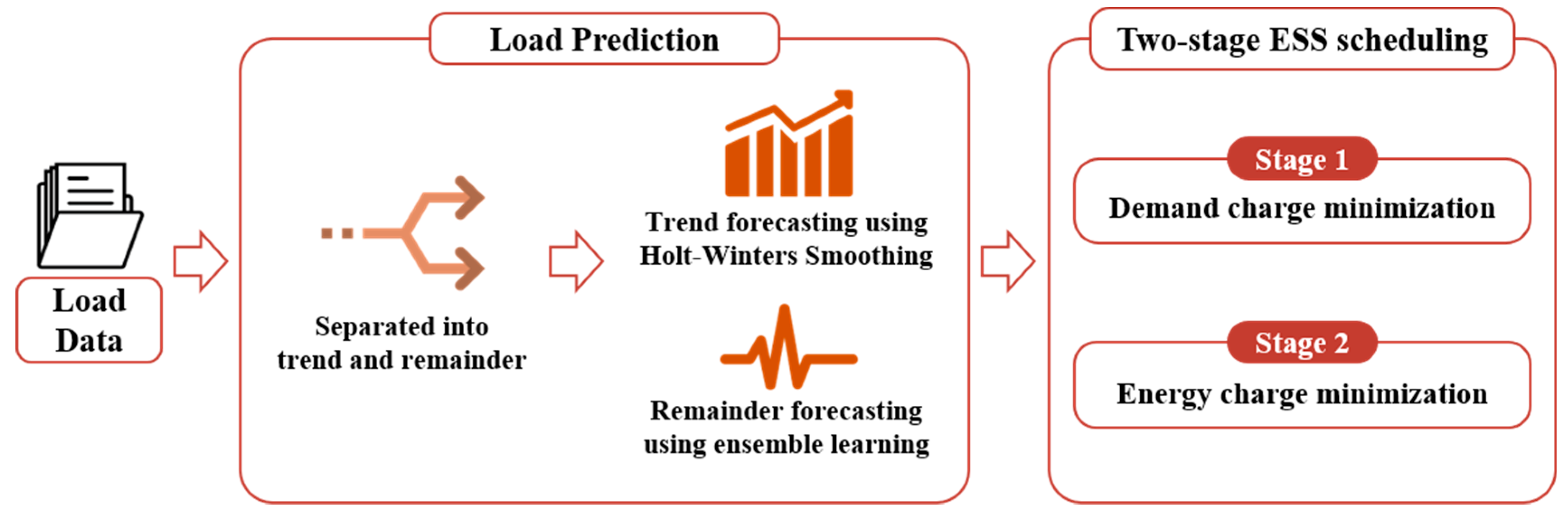
2. Load Prediction Using Ensemble Learning
2.1. Decision Tree and Feature Engineering
2.2. Bagging and Random Forest
2.3. Load Predicton Model
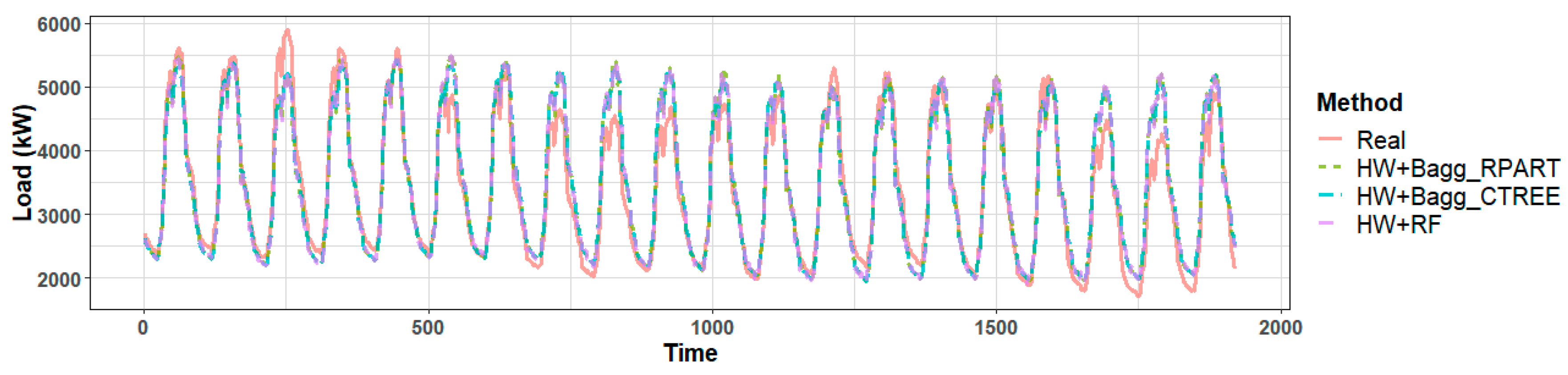
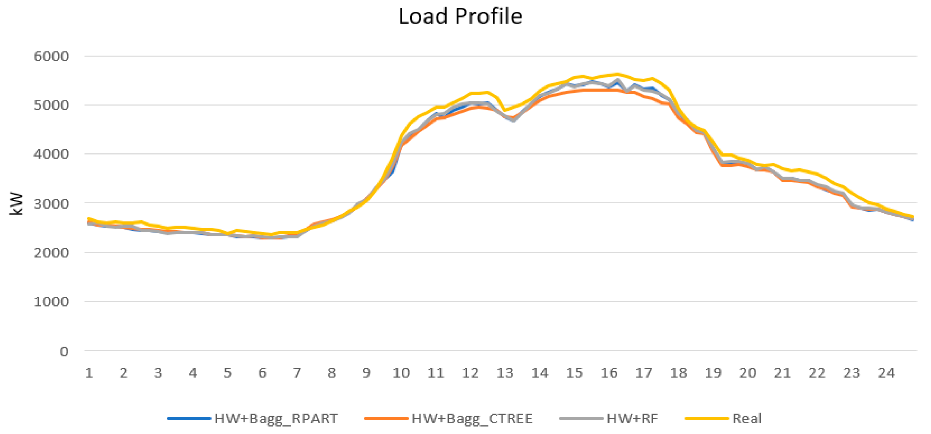
- Model 1: Holt–Winters smoothing + Bagging with RPART
- Model 2: Holt–Winters smoothing + Bagging with CTREE
- Model 3: Holt–Winters smoothing + Random Forest
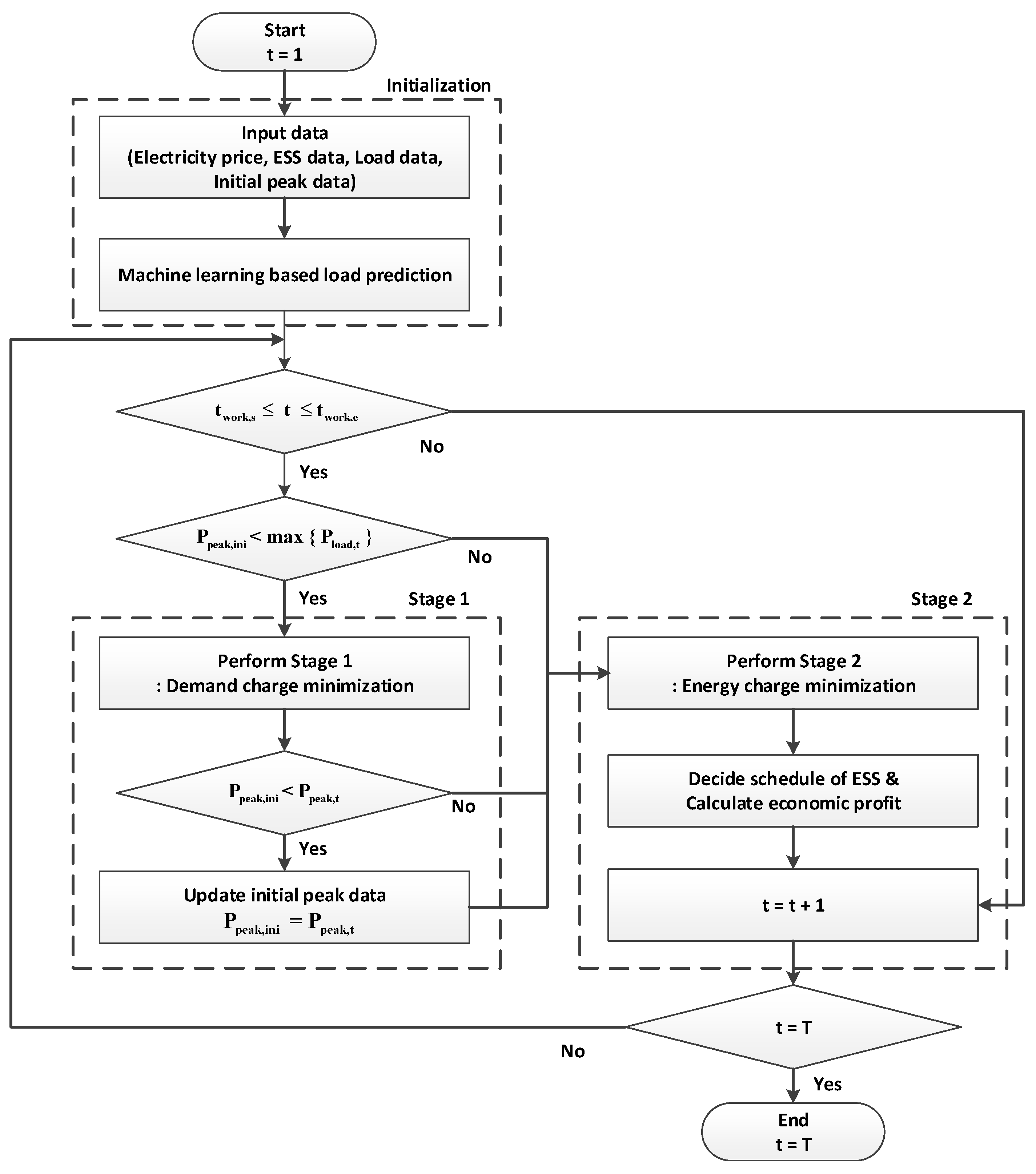
3. Two-Stage ESS-Scheduling Algorithm
3.1. ESS Optimization Model for Minimizing Demand Charges (Stage 1)
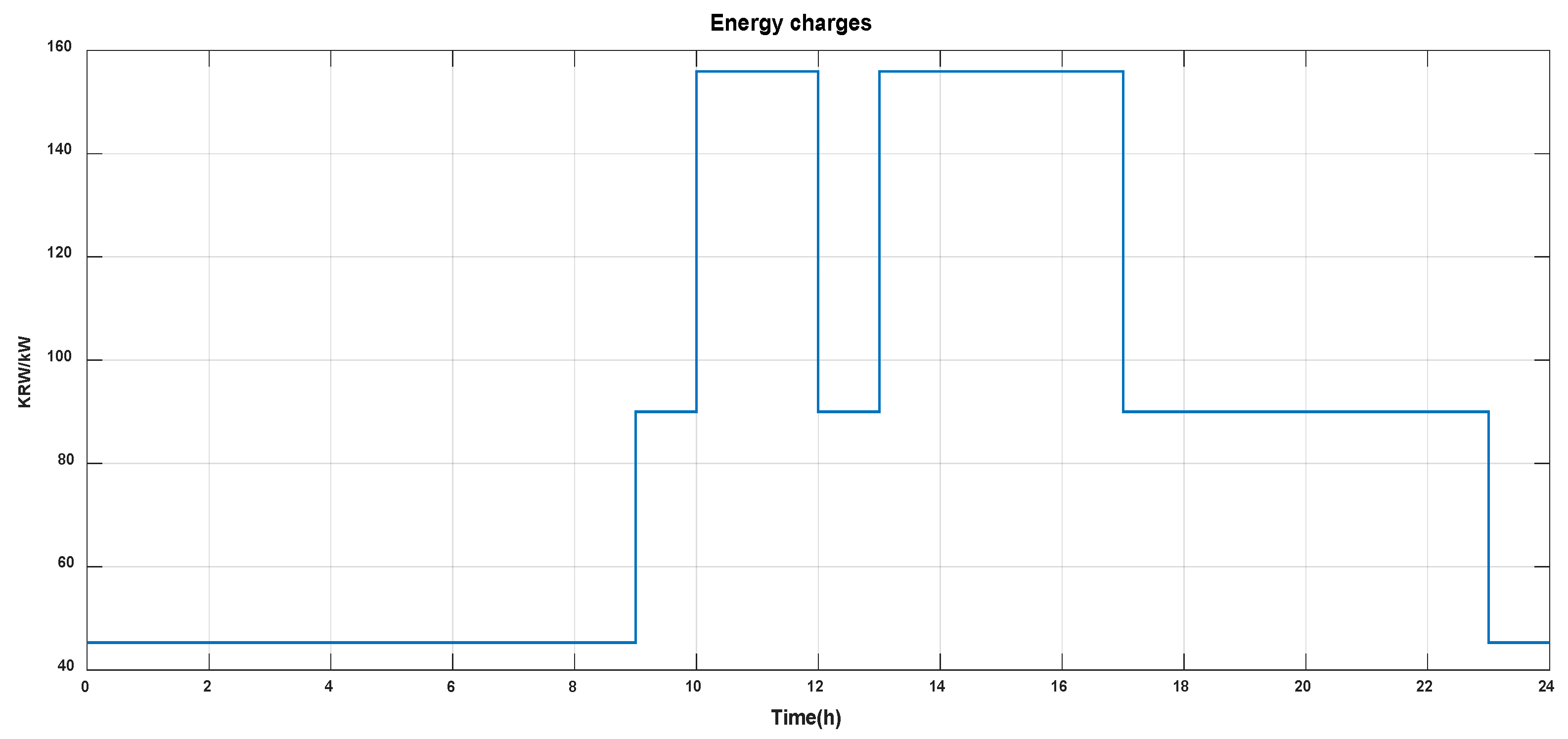
3.2. ESS Optimization Model for Minimizing Energy Charges (Stage 2)
3.3. Optimization Method for Two-Stage ESS-Scheduling
4. Case Study
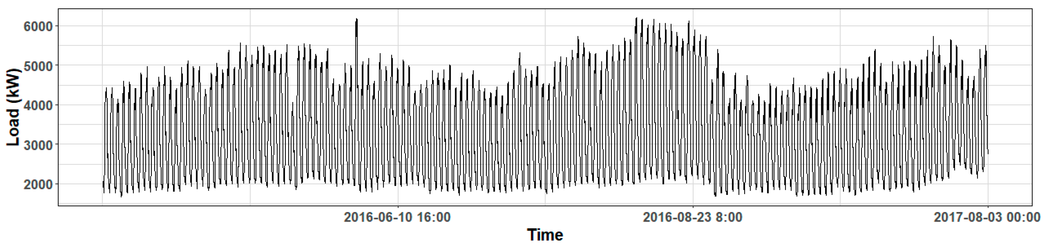
4.1. Load Data
4.2. Ensemble Learning Based Load Prediction
4.3. Results of the Two-Stage ESS-Scheduling Model Using Machine Learning Load Prediction
4.3.1. Input Parameters for the Optimization Model
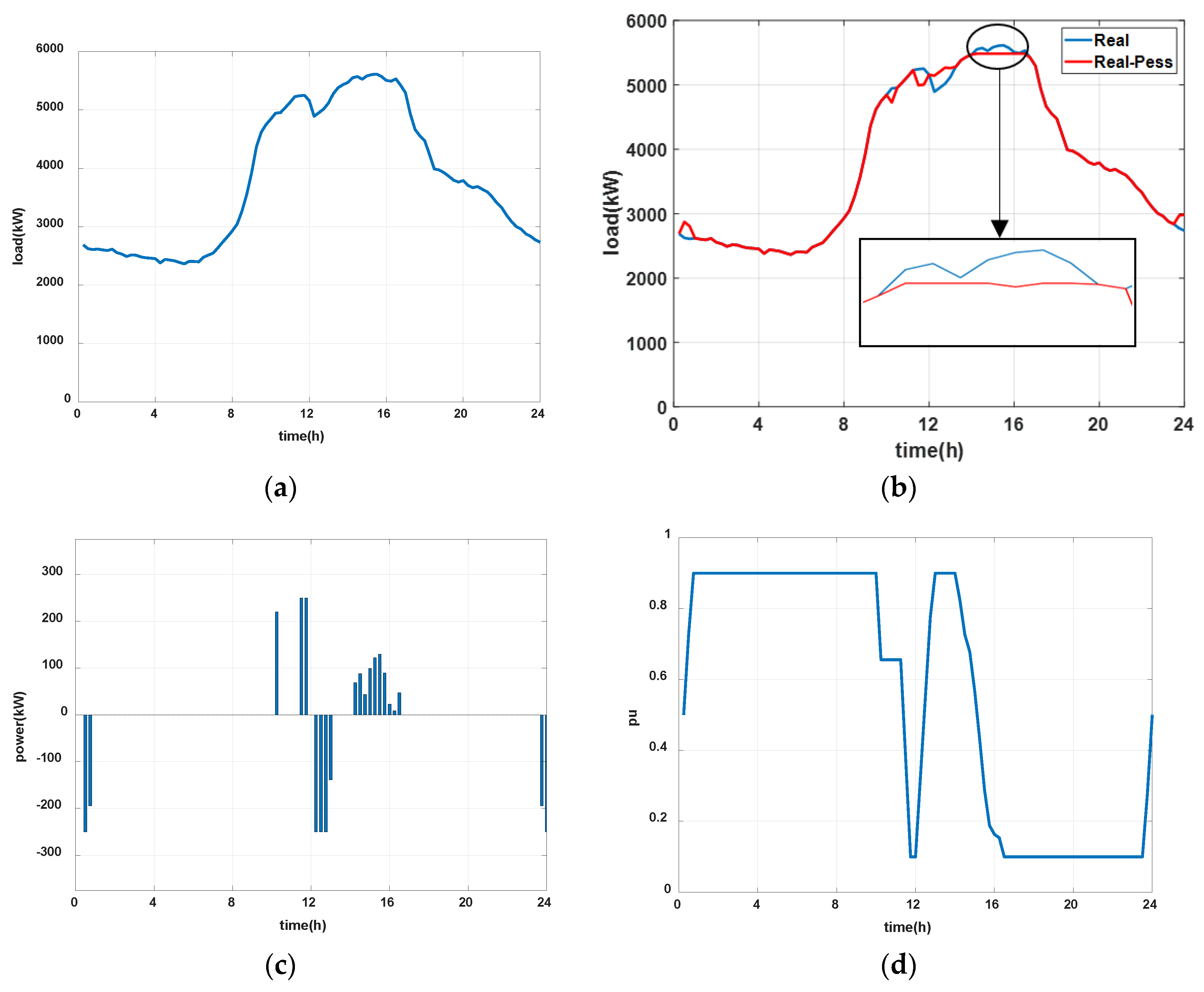
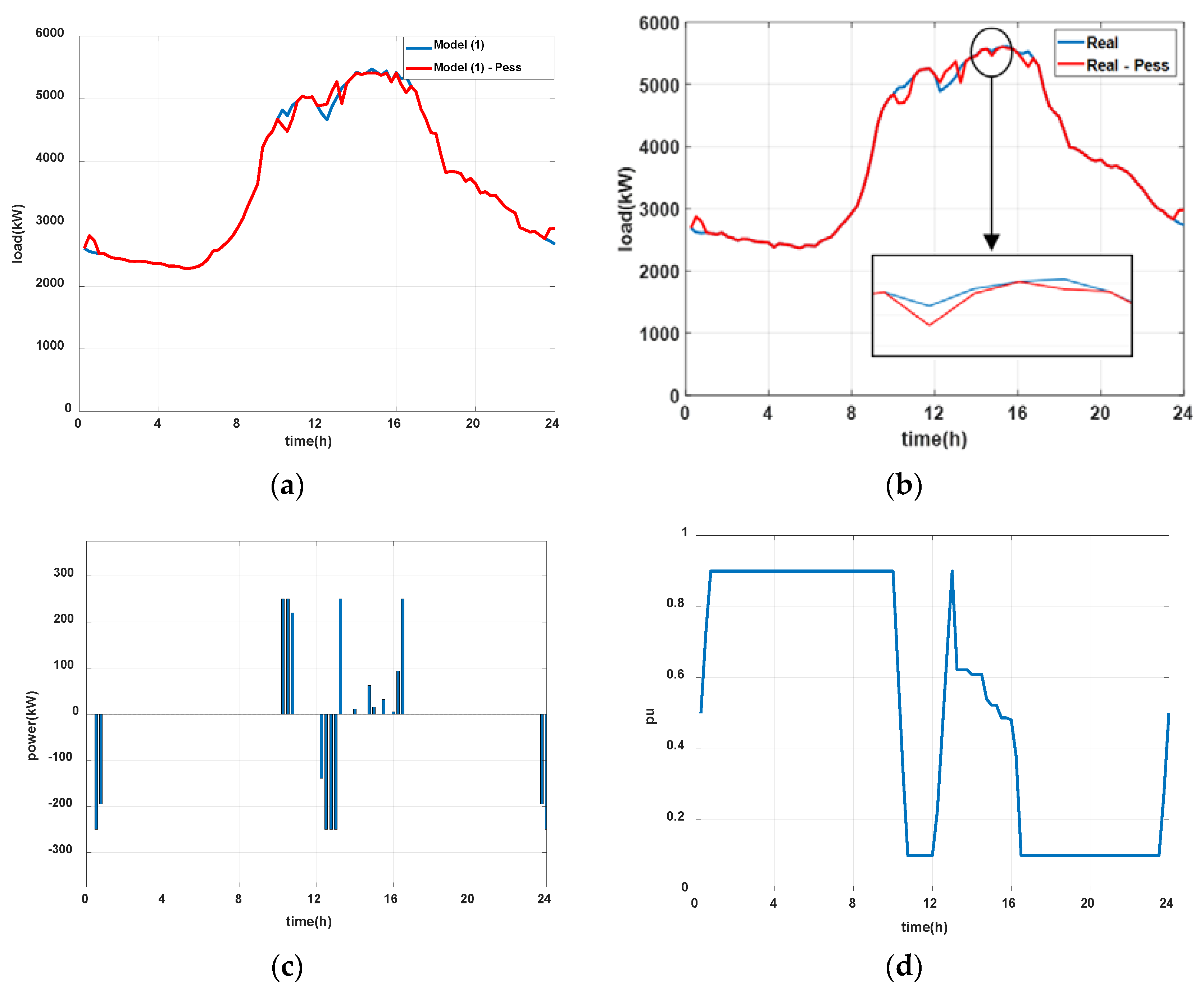
4.3.2. Two-Stage ESS-Scheduling Simulation Results
Case 1
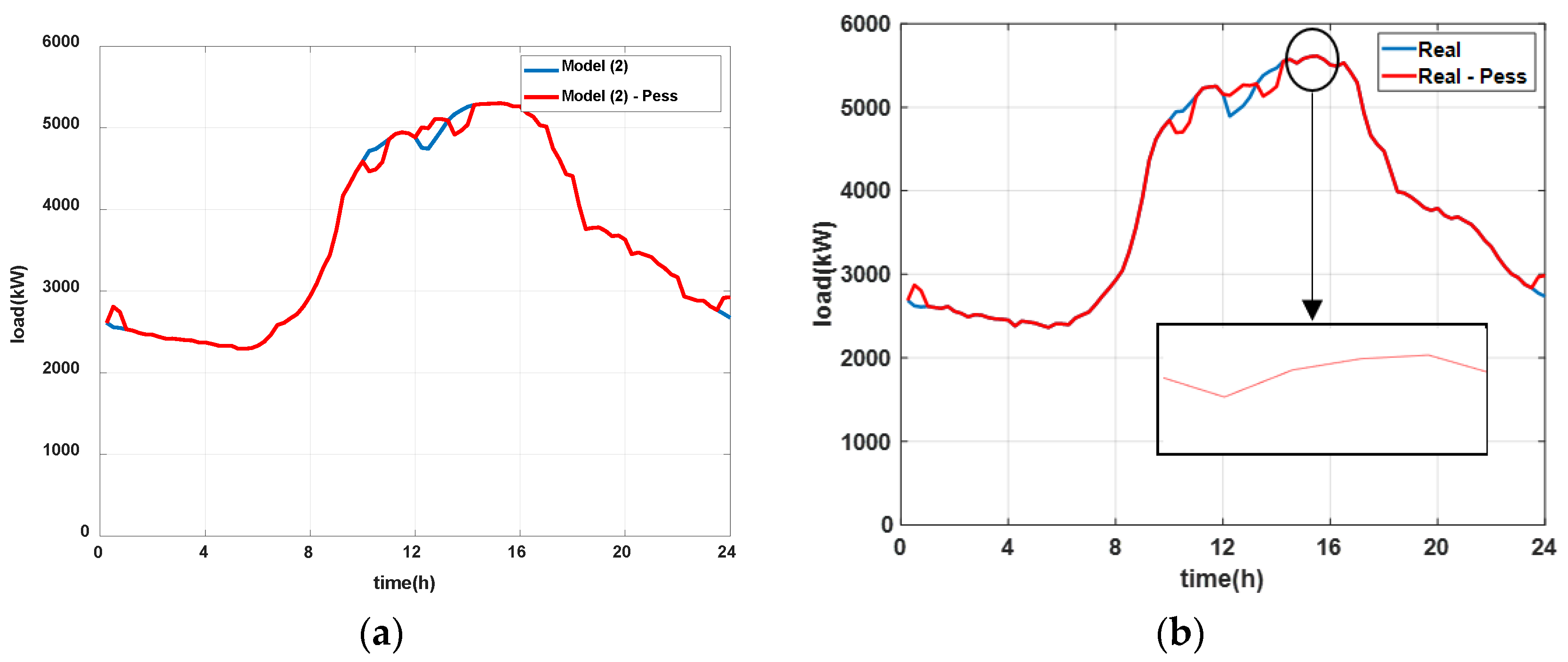
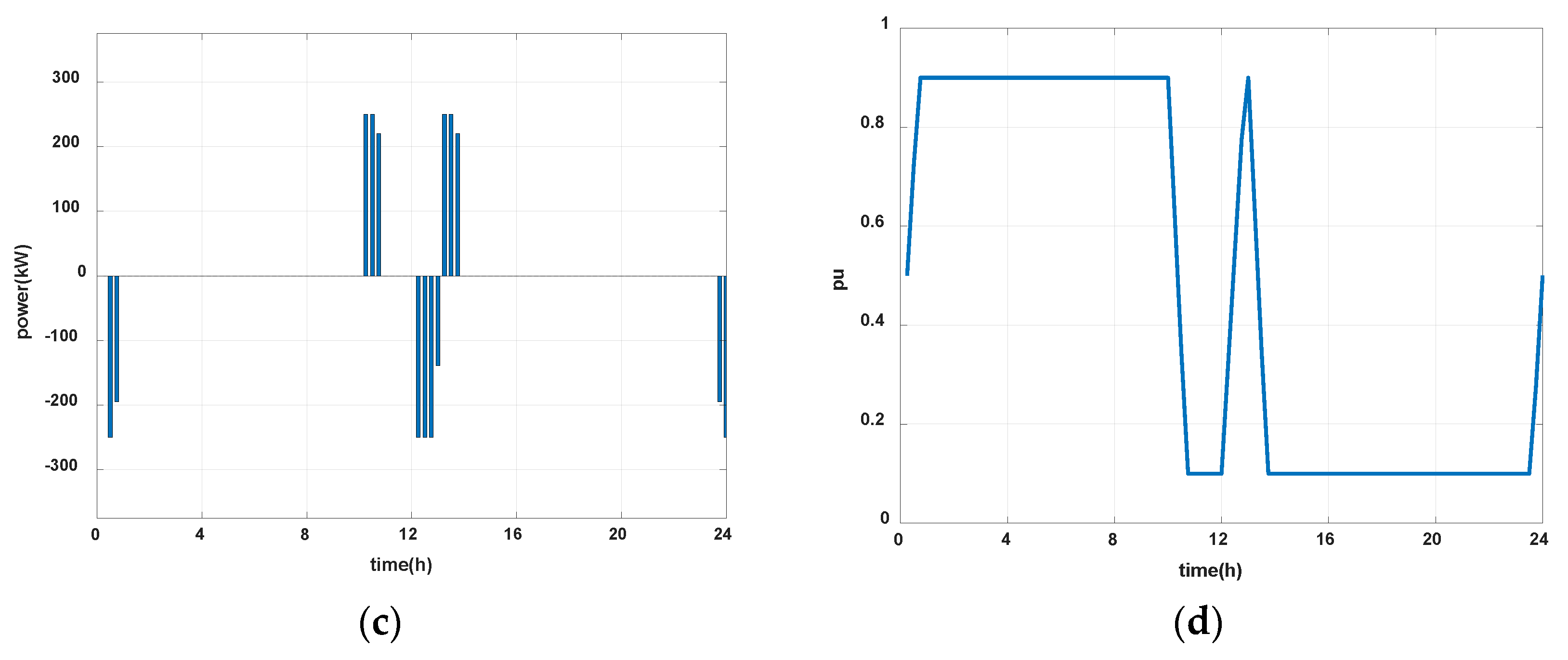
Case 2
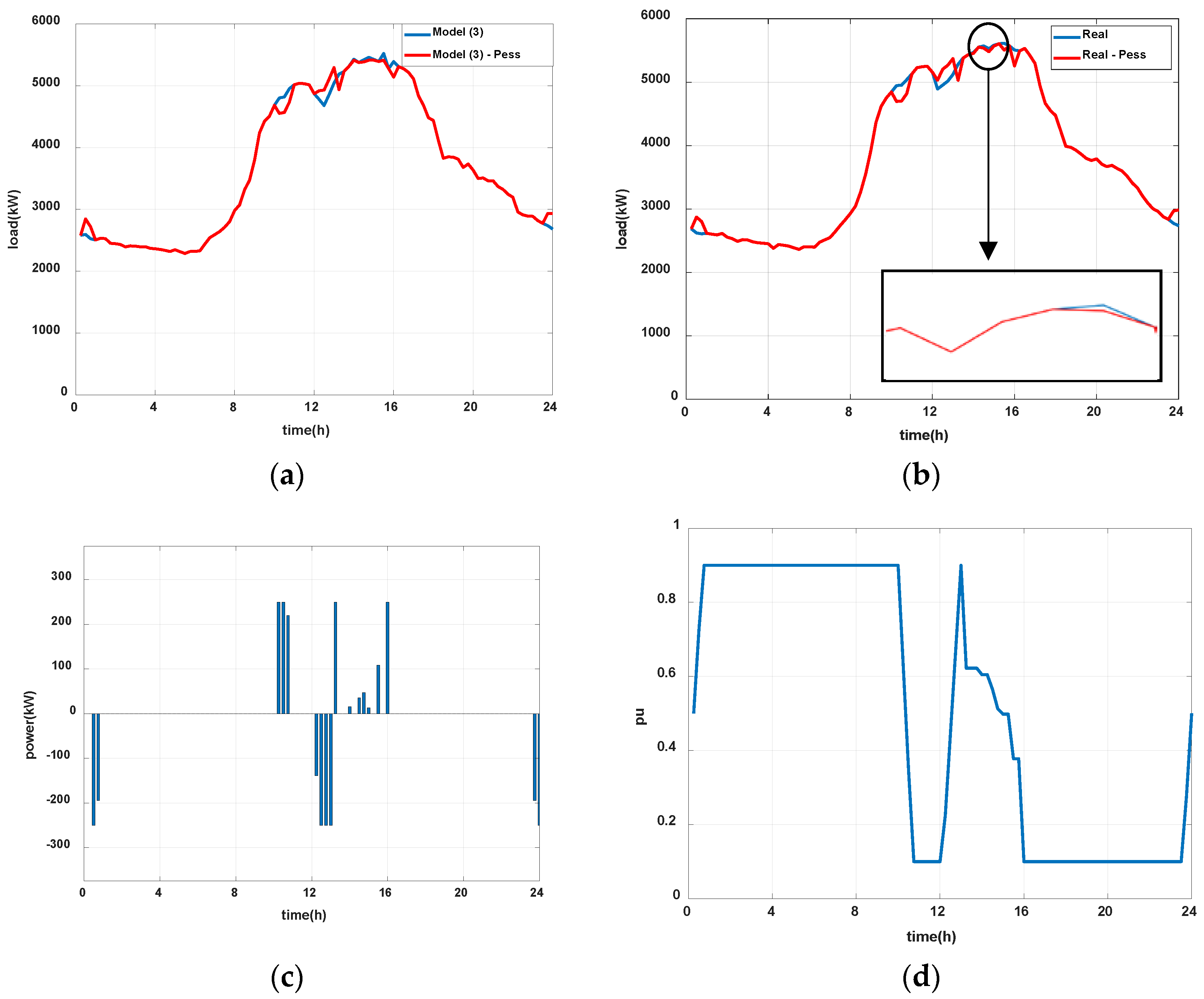
Case 3
Case 4
5. Conclusions and Future Works
Author Contributions
Funding
Acknowledgments
Conflicts of Interest
References
- UNFCCC. United Nations Climate Change. 2019. Available online: http://unfccc.int (accessed on 4 February 2019).
- Choi, S.; Choi, S.W.S.; Min, S.W. Optimal scheduling and operation of the ESS for prosumer market environment in grid-connected industrial complex. IEEE Trans. Ind. Appl. 2018, 54, 1949–1957. [Google Scholar] [CrossRef]
- Dang, J.; Seuss, J.; Suneja, L.; Harley, R.G. SOC feedback control for wind and ESS hybrid power system frequency regulation. IEEE J. Emerg. Sel. Top. Power Electron. 2014, 2, 79–86. [Google Scholar] [CrossRef]
- Faisal, M.; Hannan, M.A.; Ker, P.J.; Hussain, A.; Mansor, M.B.; Blaabjerg, F. Review of energy storage system technologies in microgrid applications: Issues and challenges. IEEE Access 2018, 7, 35143–35164. [Google Scholar] [CrossRef]
- Ke, X.; Lu, N.; Jin, C. Control and Size Energy Storage Systems for Managing Energy Imbalance of Variable Generation Resources. IEEE Trans. Sustain. Energy 2015, 6, 70–78. [Google Scholar] [CrossRef]
- Rangel, C.A.S.; Canha, L.; Sperandio, M.; Severiano, R. Methodology for ESS-type selection and optimal energy management in distribution system with DG considering reverse flow limitations and cost penalties. IET Gener. Trans. Distrib. 2017, 12, 1164–1170. [Google Scholar] [CrossRef]
- Chaudhari, K.; Ukil, A.; Kumar, K.N.; Manandhar, U.; Kollimalla, S.K. Hybrid optimization for economic deployment of ESS in PV-integrated EV charging stations. IEEE Trans. Ind. Inf. 2018, 14, 106–116. [Google Scholar] [CrossRef]
- Tang, Y.; Chen, Q.; Ning, J.; Wang, Q.; Feng, S.; Li, Y. Hierarchical control strategy for residential demand response considering time-varying aggregated capacity. Electron. Power Energy Syst. 2018, 97, 165–173. [Google Scholar] [CrossRef]
- Zhang, J.; Zhang, P.; Wu, H.; Qi, X.; Yang, S.; Li, Z. Two-stage load-scheduling model for the incentive-based demand response of industrial users considering load aggregators. IET Gener. Trans. Distrib. 2018, 12, 3518–3526. [Google Scholar] [CrossRef]
- Hong, W.C. Electric load forecasting by support vector model. Appl. Math. Model. 2009, 33, 2444–2454. [Google Scholar] [CrossRef]
- Shi, H.; Xu, M.; Li, R. Deep learning for household load forecasting—A novel pooling deep RNN. IEEE Trans. Smart Grid 2018, 9, 5271–5280. [Google Scholar] [CrossRef]
- Marino, D.L.; Amarasinghe, K.; Manic, M. Building energy load forecasting using deep neural networks. In Proceedings of the IECON 2016—42nd Annual Conference of the IEEE Industrial Electronics Society, Florence, Italy, 23–25 October 2016; pp. 7046–7051. [Google Scholar]
- Abdel-Nasser, M.; Mahmoud, K. Accurate photovoltaic power forecasting models using deep LSTM-RNN. Neural Comput. Appl. 2017, 28, 1–14. [Google Scholar] [CrossRef]
- Grmanová, G.; Laurinec, P.; Rozinajová, V.; Ezzeddine, A.B.; Lucká, M.; Lacko, P.; Návrat, P. Incremental ensemble learning for electricity load forecasting. Acta Polytechnica Hungarica 2016, 13, 97–117. [Google Scholar]
- Laurinec, P. Ensemble Learning for Time Series Forecasting in R. 2017. Available online: https://petolau.github.io/Ensemble-of-trees-for-forecasting-time-series/ (accessed on 10 August 2018).
- Zang, W.; Zhang, P.; Zhou, C.; Guo, L. Comparative study between incremental and ensemble learning on data streams: Case study. J. Big Data 2014, 1, 5. [Google Scholar] [CrossRef]
- James, G.; Witten, D.; Hastie, T.; Tibshirani, R. (Eds.) An Introduction to Statistical Learning; Springer: New York, NY, USA, 2013. [Google Scholar]
- Hastie, T.; Tibshirani, R.; Fridman, J. (Eds.) The Elements of Statistical Learning; Springer: New York, NY, USA, 2001. [Google Scholar]
- Therneau, T.M.; Atkinson, E.J. An Introduction to Recursive Partitioning Using the RPART Routines; Technical Report; Mayo Foundation: Rochester, MN, USA, 1997. [Google Scholar]
- Hothorn, T.; Hornik, K.; Zeileis, A. Party: A laboratory for recursive part(y)itioning. 2010. Available online: http://citeseerx.ist.psu.edu/viewdoc/summary?doi=10.1.1.151.2872 (accessed on 10 February 2019).
- Deshpande, B. Learning Data Science: Feature Engineering. 2016. Available online: http://www.simafore.com/blog/learning-data-science-feature-engineering (accessed on 10 February 2019).
- Brownlee, J. Discover Feature Engineering, How to Engineer Features and How to Get Good at It. 2014. Available online: https://machinelearningmastery.com/discover-feature-engineering-how-to-engineer-features-and-how-to-get-good-at-it/ (accessed on 10 February 2019).
- Cowpertwait, P.S.P.; Metcalfe, A.V. (Eds.) Introductory Time Series with R; Springer: New York, NY, USA, 2009. [Google Scholar]
- Breiman, L. Bagging predictors. Mach. Learn. 1996, 24, 123–140. [Google Scholar] [CrossRef] [Green Version]
- KEPCO. Electric Rates Table. 2019. Available online: http://cyber.kepco.co.kr/ckepco/front/jsp/CY/E/E/CYEEHP00201.jsp (accessed on 11 January 2019).
- Rao, S.S. (Ed.) Engineering Optimization: Theory and Practice; John Wiley & Sons, Inc.: Hoboken, NJ, USA, 2009. [Google Scholar]


| Model. | RMSE | MAE | MAPE (%) |
|---|---|---|---|
| Model 1 | 299.3747 | 227.1160 | 6.740471 |
| Model 2 | 296.4163 | 225.8964 | 6.704895 |
| Model 3 | 299.9798 | 227.8008 | 6.771545 |
| DNN model | 526.2574 | 419.8826 | 12.991492 |
| Parameter | Definition | Value | Parameter | Definition | Value |
|---|---|---|---|---|---|
| Demand Charges | 6980 KRW/kW | Initial Peak | 5412.15 | ||
| Charging Efficiency | 90% | Maximum SOC | 0.9 | ||
| Discharging Efficiency | 90% | Minimum SOC | 0.1 | ||
| Discharge Rated Power | 250 kW | Initial SOC | 0.5 | ||
| Charge Rated Power | 250 kW | Final SOC | 0.5 |
| Case | Simulation Conditions | |
|---|---|---|
| Load Data | Peak Load | |
| Case 1 | Real | 5614.08 kW |
| Case 2 | HW + Bagg_RPART (Model 1) | 5474.60 kW |
| Case 3 | HW + Bagg_CTREE (Model 2) | 5302.70 kW |
| Case 4 | HW+RF (Model 3) | 5520.52 kW |
| Case | Simulation Results | ||
|---|---|---|---|
| Demand Charges | Energy Charges | Total Reduction Rate | |
| Base Case | 39,186,000 KRW | 9,132,015 KRW/kW | - |
| Case 1 | 38,279,000 KRW | 9,106,000 KRW/kW | 933,015 KRW |
| Case 2 | 39,132,672 KRW | 9,106,000 KRW/kW | 79,343 KRW |
| Case 3 | 39,186,000 KRW | 9,106,000 KRW/kW | 26,015 KRW |
| Case 4 | 39,132,672 KRW | 9,106,000 KRW/kW | 79,343 KRW |
© 2019 by the authors. Licensee MDPI, Basel, Switzerland. This article is an open access article distributed under the terms and conditions of the Creative Commons Attribution (CC BY) license (http://creativecommons.org/licenses/by/4.0/).
Share and Cite
Park, M.; Kim, J.; Won, D.; Kim, J. Development of a Two-Stage ESS-Scheduling Model for Cost Minimization Using Machine Learning-Based Load Prediction Techniques. Processes 2019, 7, 370. https://doi.org/10.3390/pr7060370
Park M, Kim J, Won D, Kim J. Development of a Two-Stage ESS-Scheduling Model for Cost Minimization Using Machine Learning-Based Load Prediction Techniques. Processes. 2019; 7(6):370. https://doi.org/10.3390/pr7060370
Chicago/Turabian StylePark, Minsu, Jaehwi Kim, Dongjun Won, and Jaehee Kim. 2019. "Development of a Two-Stage ESS-Scheduling Model for Cost Minimization Using Machine Learning-Based Load Prediction Techniques" Processes 7, no. 6: 370. https://doi.org/10.3390/pr7060370