Impact of Thermal Radiation on Magnetohydrodynamic Unsteady Thin Film Flow of Sisko Fluid over a Stretching Surface


Abstract
:1. Introduction
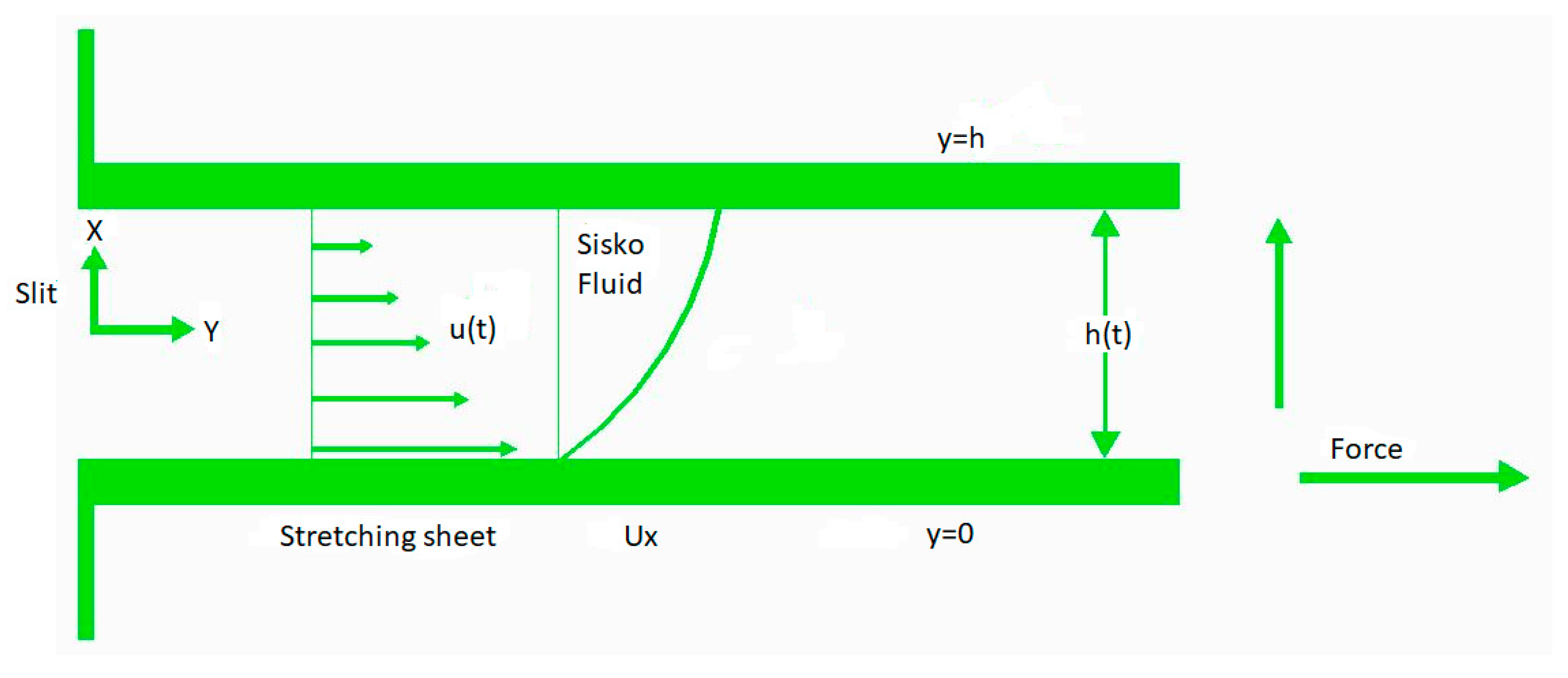
2. Basic Equations
3. Mathematical Formulation of the Problem
Similarity Transformations
4. Application of Homotopy Analysis Method
4.1. Zeroth rder Deformation Problem
4.2. ith-Order Deformation Problem
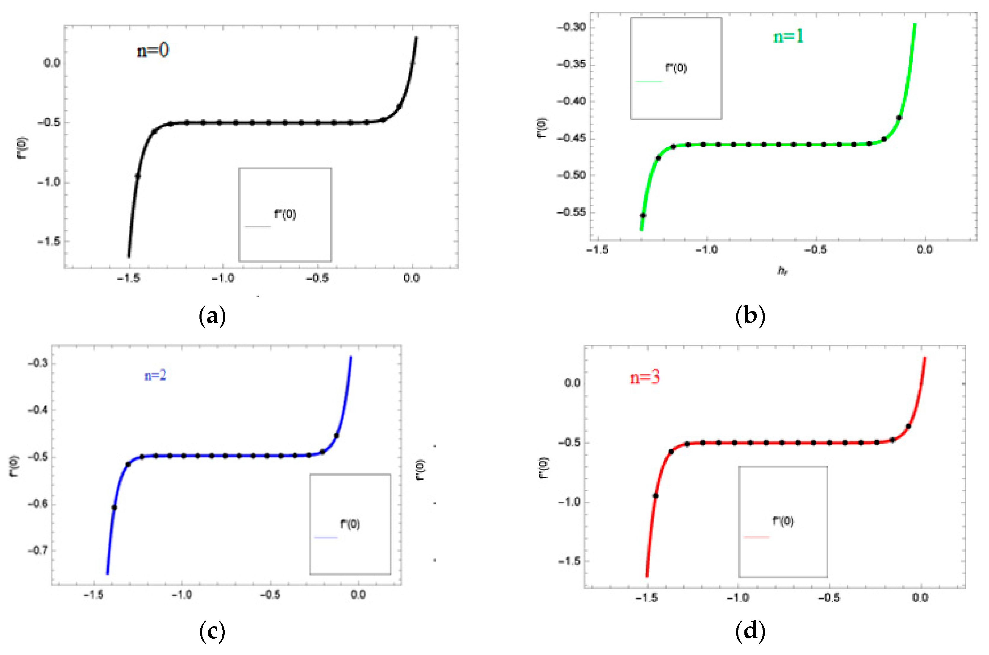
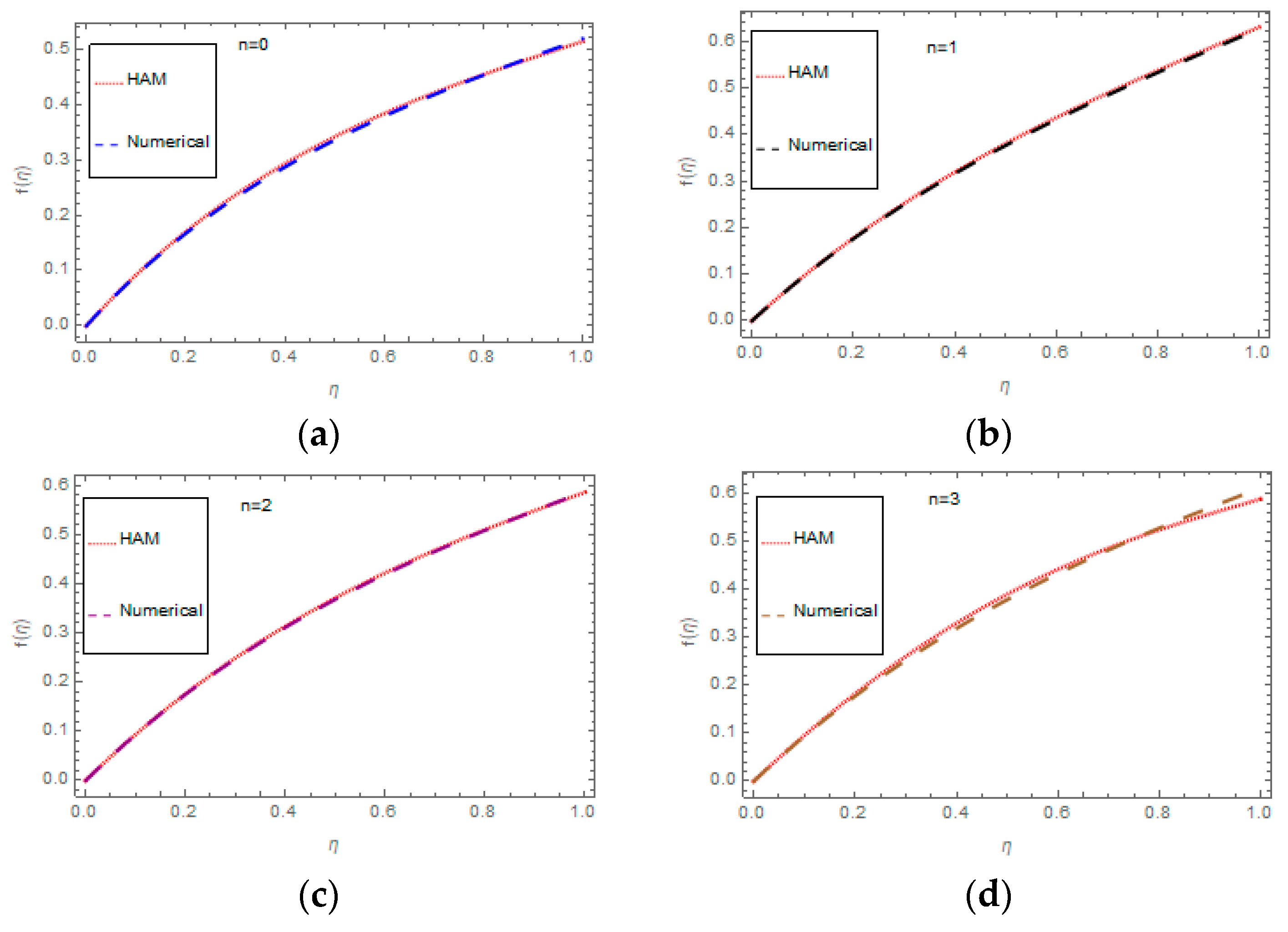
4.3. Convergence of Solution
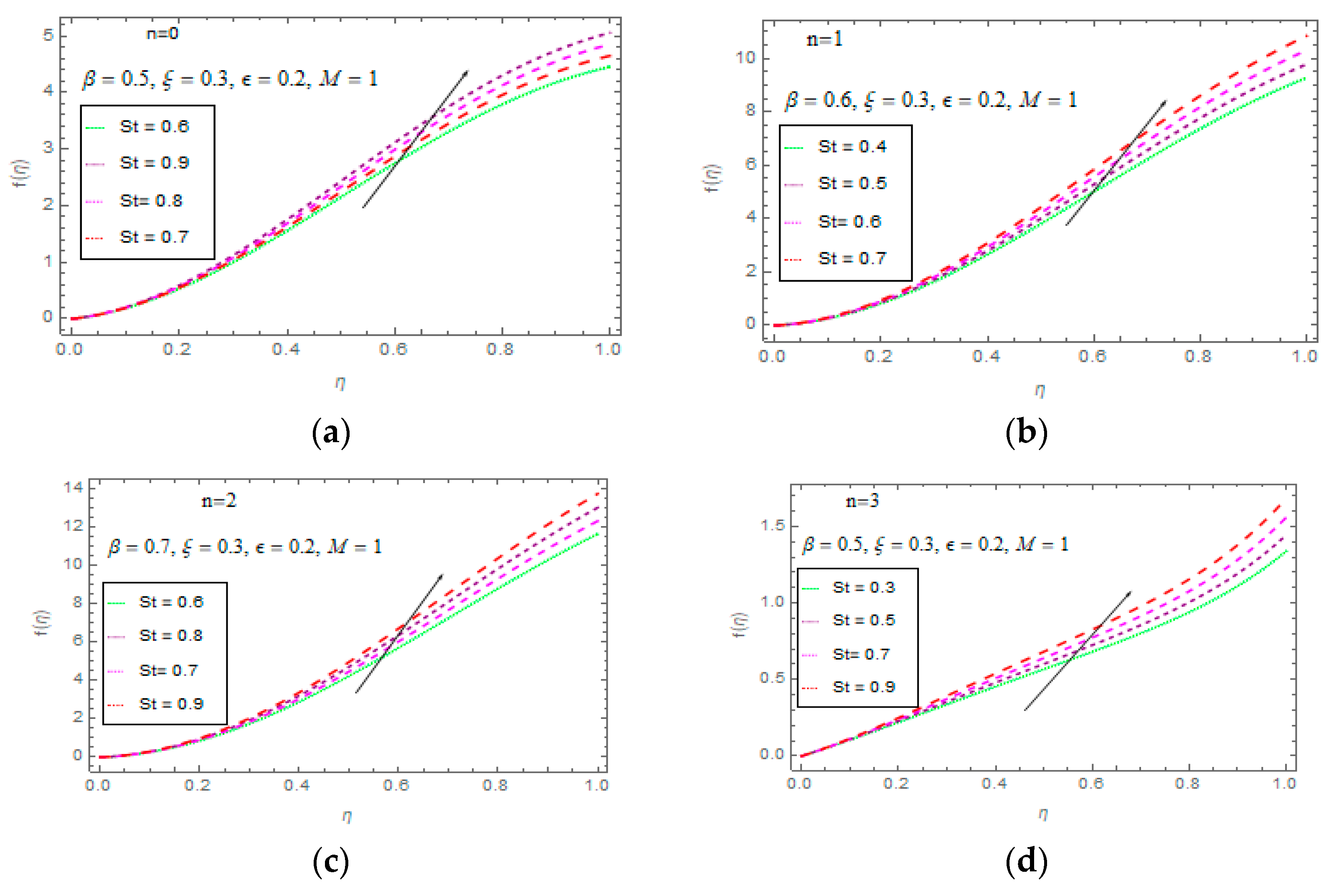
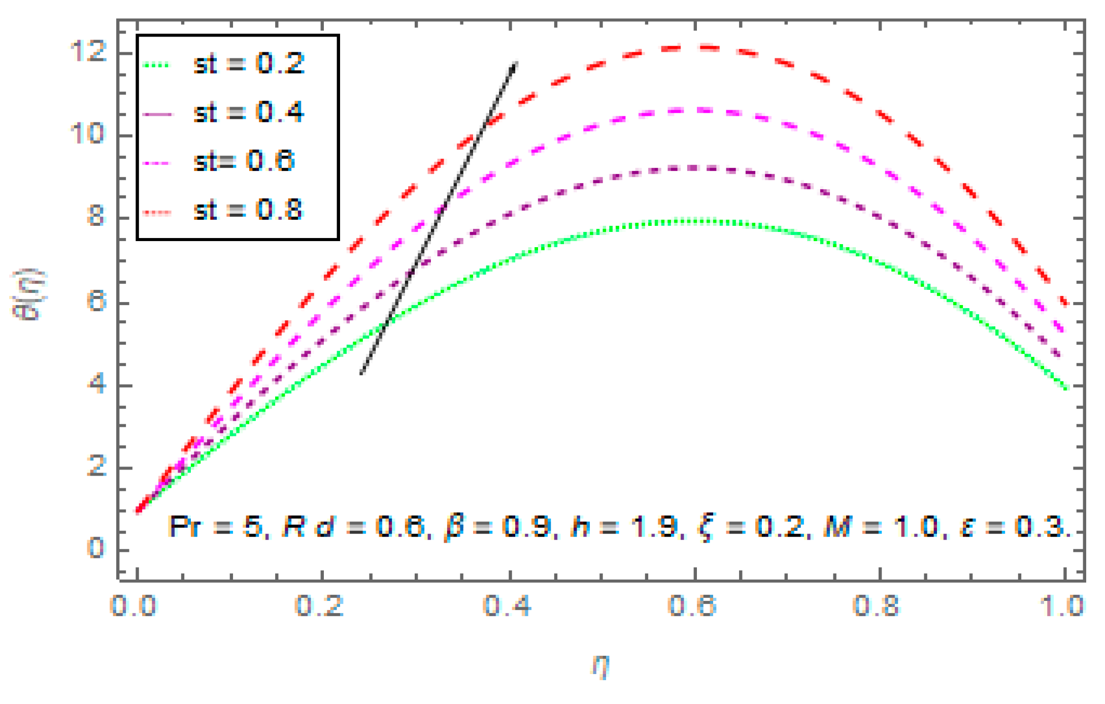
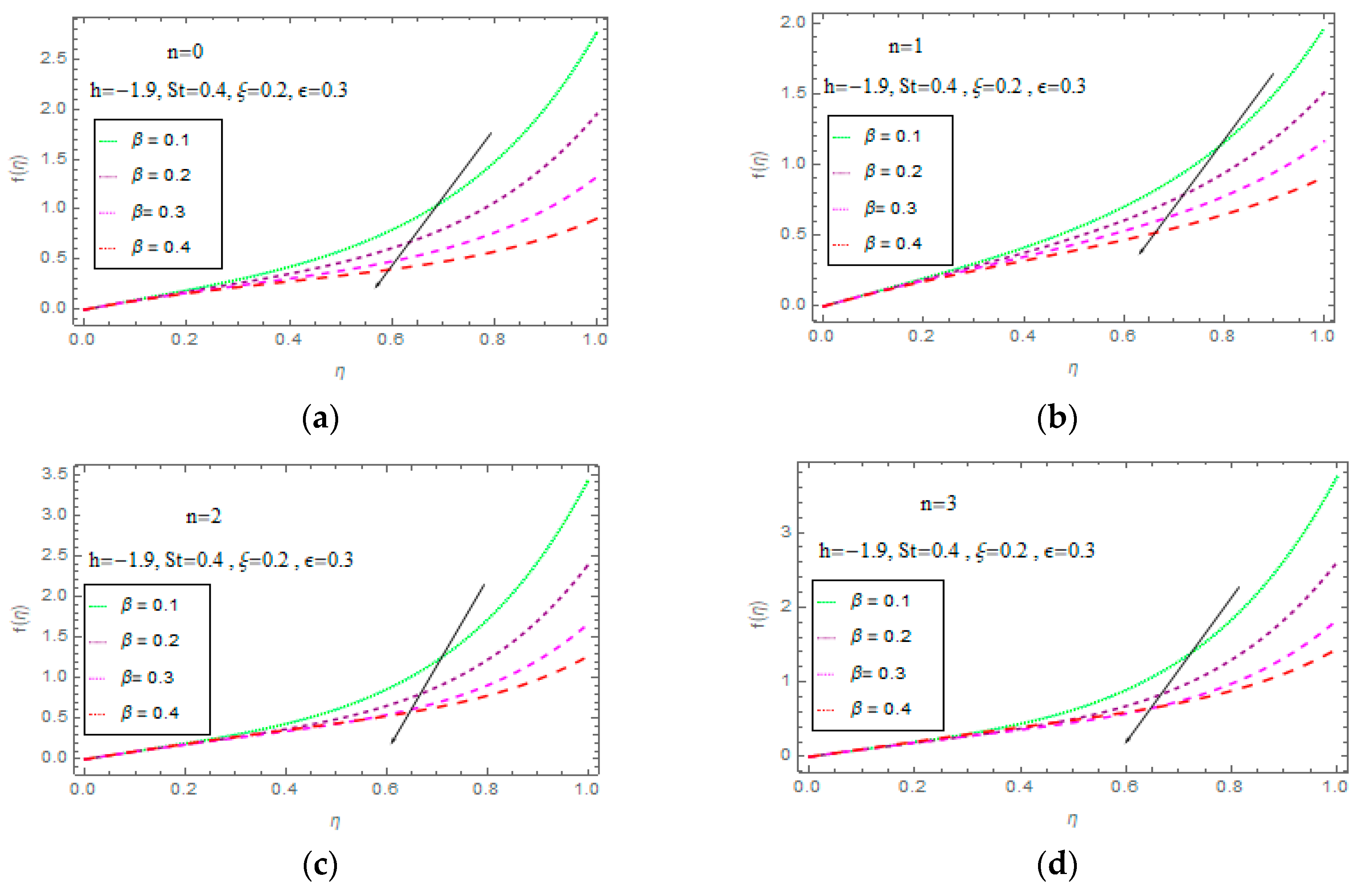
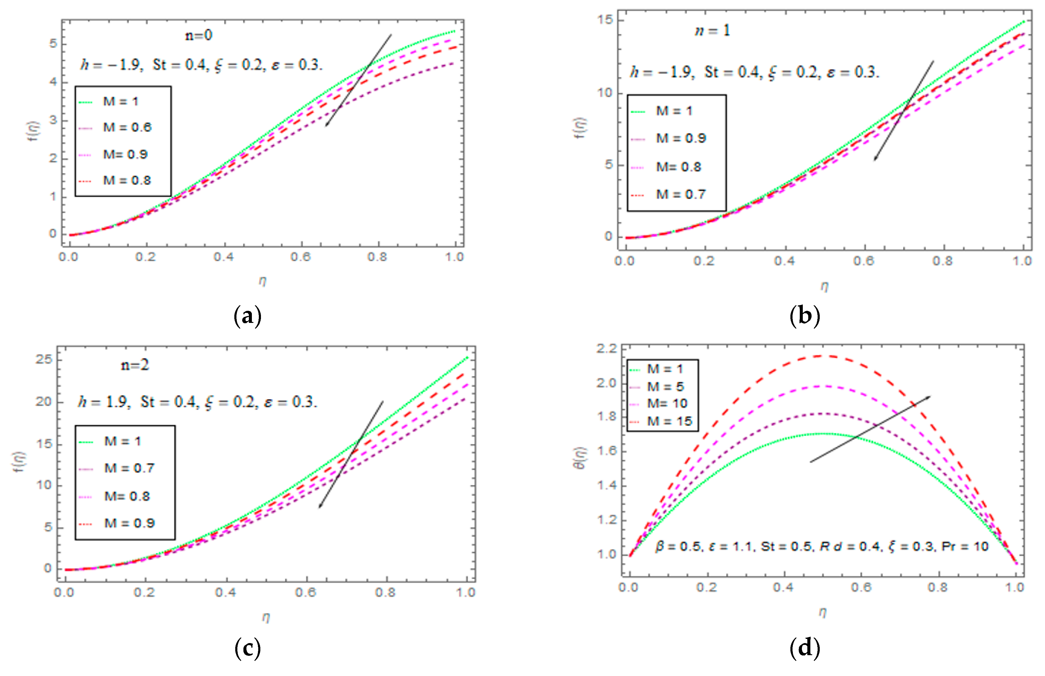
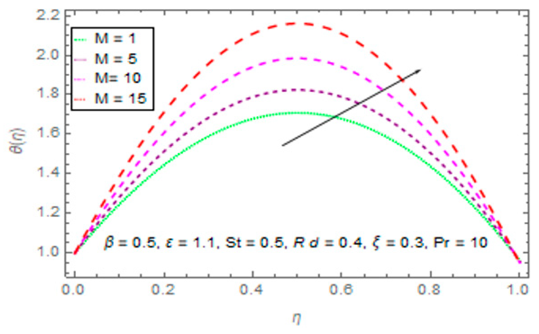
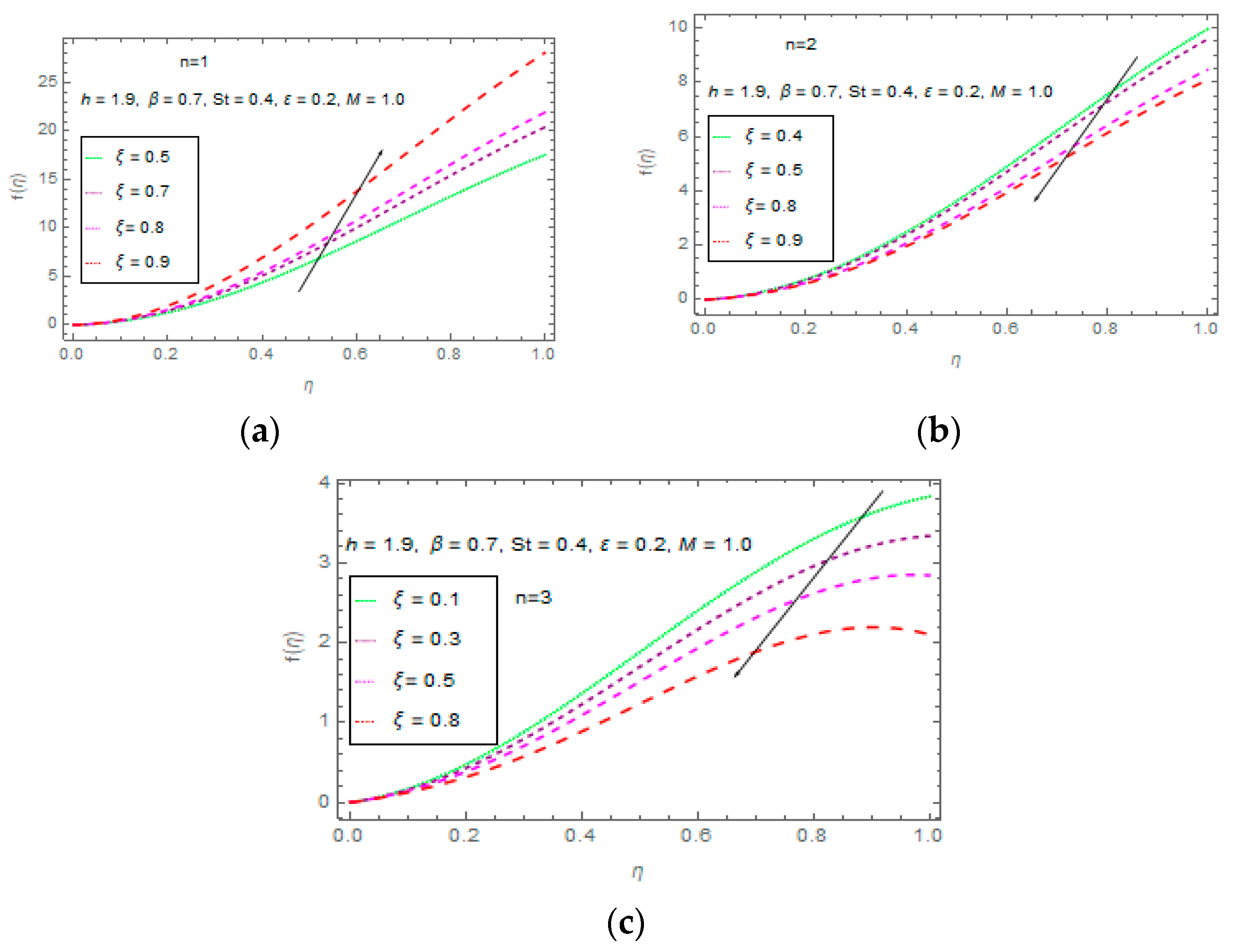
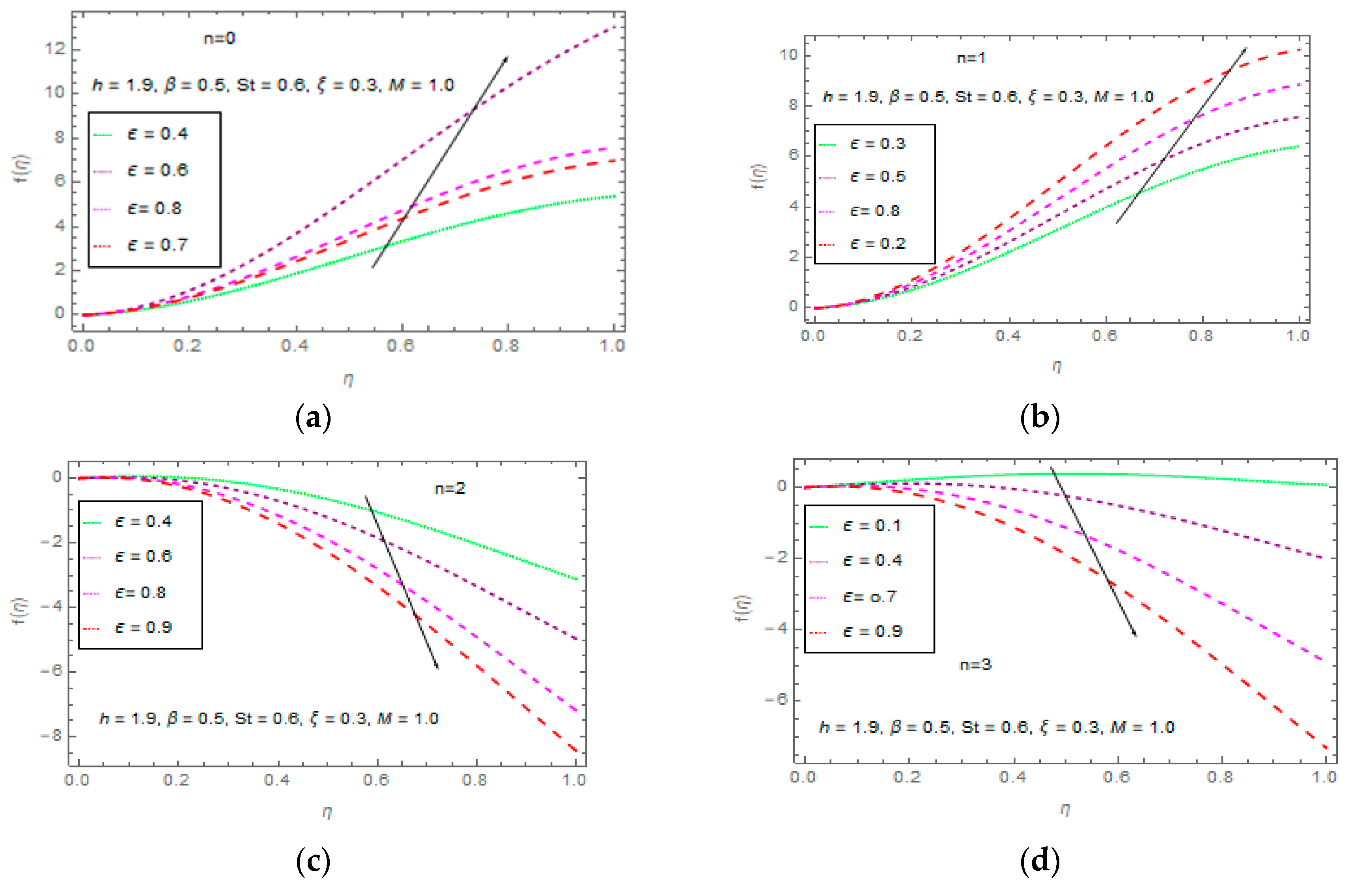
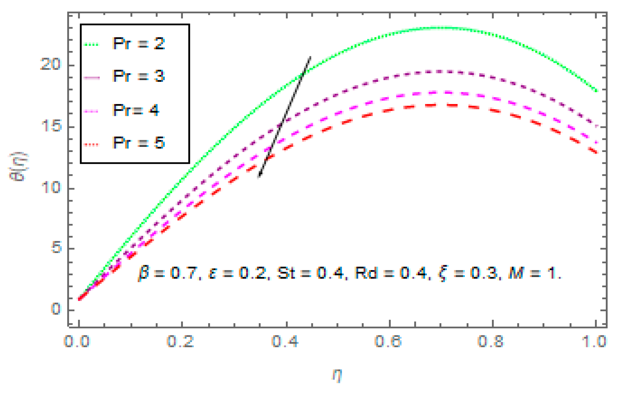
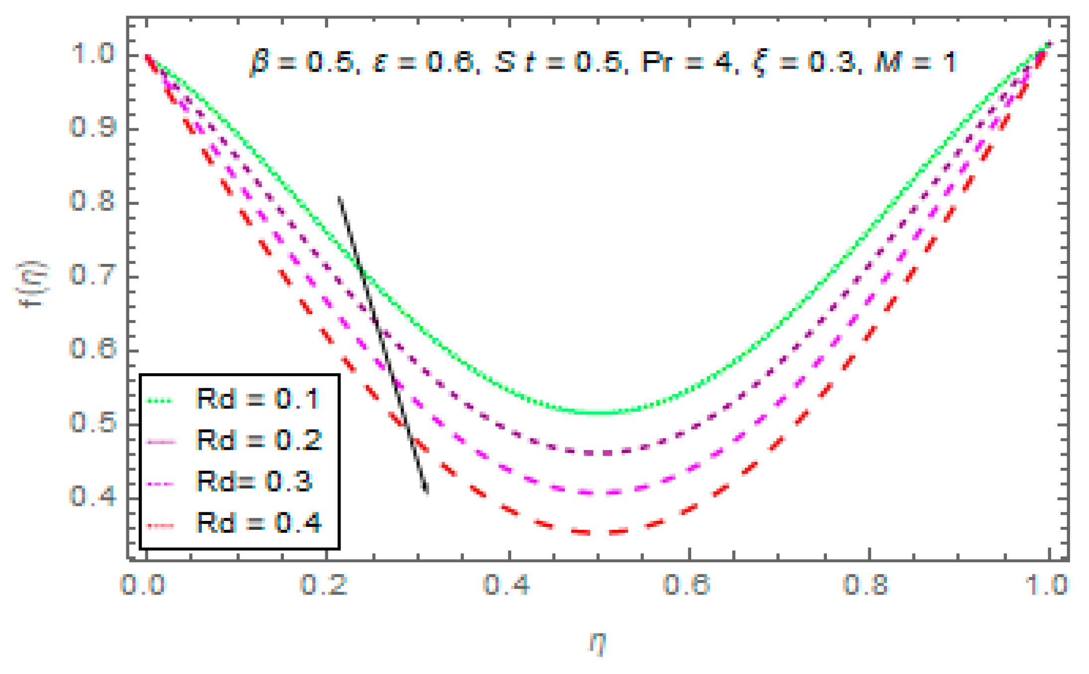
5. Results and Discussion
Table Discussion
6. Conclusions
- ⮚
- In the present investigation we see that due to greater value of magnetic parameter, the velocity distribution of the thin films fluid will be decreasing.
- ⮚
- Increasing thin film thickness decreases the motion of the fluid
- ⮚
- Due to increasing radiation parameters, the Nusselt number increases.
- ⮚
- The increasing values of Pr number, raising the temperature of the surface, also caused the surface temperature to fall down for large values of unsteady parameters.
- ⮚
- The effect of the liquid film flow on the flow of Sisko fluids has been studied graphically and also shown in tables.
- ⮚
- At the end it is also summarized that due to the Lorentz’s force the liquid film flow is affected.
- ⮚
- The Sisko fluid parameter increases velocity field.
- ⮚
- The effect of all parameters is shown for dissimilar values of power index and .
Author Contributions
Funding
Conflicts of Interest
References
- Crane, L.J. Flow past a stretching plate. Angrew. Math. Phys. 1970, 21, 645–647. [Google Scholar] [CrossRef]
- Dandapat, B.S.; Gupta, A.S. Flow and heat transfer in a viscoelastic fluid over a stretching sheet. Int. J. Nonlinear Mech. 1989, 24, 215–219. [Google Scholar] [CrossRef]
- Wang, C.Y. Liquid film on an unsteady stretching surface. Q. Appl. Math. 1990, 48, 601–610. [Google Scholar] [CrossRef] [Green Version]
- Usha, R.; Sridharan, R. On the motion of a liquid film on an unsteady stretching surface. ASME Fluids Eng. 1993, 150, 43–48. [Google Scholar] [CrossRef]
- Liu, I.C.; Andersson, I.H. Heat transfer in a liquid film on an unsteady stretching sheet. Int. J. Therm. Sci. 2008, 47, 766–772. [Google Scholar] [CrossRef]
- Aziz, R.C.; Hashim, I.; Alomari, A.K. Thin film flow and heat transfer on an unsteady stretching sheet with internal heating. Meccanica 2011, 46, 349–357. [Google Scholar] [CrossRef]
- Tawade, L.; Abel, M.; GMetri, P.; Koti, A. Thin filmflow and heat transfer over an unsteady stretching sheet with thermal radiation, internal heating in presence of external magnetic field. Int. J. Adv. Appl. Math. Mech. 2016, 3, 29–40. [Google Scholar]
- Andersson, H.I.; Aarseth, J.B.; Braud, N.; Dandapat, B.C. Flow of a power-law fluid film on an unsteady stretching surface. J. Non-Newton. Fluid Mech. 1996, 62, 1–8. [Google Scholar] [CrossRef]
- Waris, K.; Gul, T.; Idrees, M.; Islam, S.; Khan, I.; Dennis, L.C.C. Thin FilmWilliamson Nanofluid Flow with Varying Viscosity and Thermal Conductivity on a Time-Dependent Stretching Sheet. Appl. Sci. 2016, 6, 334. [Google Scholar]
- Anderssona, H.I.; Aarseth, J.B.; Dandapatb, B.C. Heat transfer in a liquid film on an unsteady stretching. Int. J. Heat Mass Transf. 2000, 43, 69–74. [Google Scholar] [CrossRef]
- Chen, C.H. Heat transfer in a power-law liquid fillm over a unsteady stretching sheet. Heat Mass Transf. 2003, 39, 791–796. [Google Scholar] [CrossRef]
- Chen, C.H. Effect of viscous dissipation on heat transfer in a non-Newtonian liquid film over an unsteady stretching sheet. J. Non-Newton. Fluid Mech. 2006, 135, 128–135. [Google Scholar] [CrossRef]
- Wang, C.; Pop, L. Analysis of the flow of a power-law liquid film on an unsteady stretching surface by means of homotopy analysis method. J. Non-Newton. Fluid Mech. 2006, 138, 161–172. [Google Scholar] [CrossRef]
- Saeed, A.; Shah, Z.; Islam, S.; Jawad, M.; Ullah, A.; Gul, T.; Kumam, P. Three-Dimensional Casson Nanofluid Thin Film Flow over an Inclined Rotating Disk with the Impact of Heat Generation/Consumption and Thermal Radiation. Coatings 2019, 9, 248. [Google Scholar] [CrossRef]
- Shah, Z.; Dawar, A.; Kumam, P.; Khan, W.; Islam, S. Impact of Nonlinear Thermal Radiation on MHD Nanofluid Thin Film Flow over a Horizontally Rotating Disk. Appl. Sci. 2019, 9, 1533. [Google Scholar] [CrossRef]
- Khan, N.S.; Gul, T.; Kumam, P.; Shah, Z.; Islam, S.; Khan, W.; Zuhra, S.; Sohail, A. Influence of Inclined Magnetic Field on Carreau Nanoliquid Thin Film Flow and Heat Transfer with Graphene Nanoparticles. Energies 2019, 12, 1459. [Google Scholar] [CrossRef]
- Khan, N.S.; Zuhra, S.; Shah, Z.; Bonyah, E.; Khan, W.; Islam, S. Slip flow of Eyring-Powell nanoliquid film containing graphene nanoparticles. AIP Adv. 2018, 8, 115302. [Google Scholar] [CrossRef]
- Ullah, A.; Alzahrani, E.O.; Shah, Z.; Ayaz, M.; Islam, S. Nanofluids Thin Film Flow of Reiner-Philippoff Fluid over an Unstable Stretching Surface with Brownian Motion and Thermophoresis Effects. Coatings 2019, 9, 21. [Google Scholar] [CrossRef]
- Shah, Z.; Bonyah, E.; Islam, S.; Khan, W.; Ishaq, M. Radiative MHD thin film flow of Williamson fluid over an unsteady permeable stretching. Heliyon 2018, 4, e00825. [Google Scholar] [CrossRef] [PubMed]
- Isko, A. The flow of lubricating greases. Ind. Eng. Chem. 1958, 50, 1789–1792. [Google Scholar]
- Siddiqui, A.; Ahmed, M.; Ghori, Q. Thin film flow of non-newtonian fluids on a moving belt. Chaos Solitons Fractals 2007, 33, 1006–1016. [Google Scholar] [CrossRef]
- Siddiqui, A.; Ashraf, H.; Walait, A.; Haroon, T. On study of horizontal thin film flow of sisko fluid due to surface tension gradient. Appl. Math. Mech. 2015, 36, 847–862. [Google Scholar] [CrossRef]
- Khan, M.; Shahzad, A. On boundary layer flow of a Sisko fluid over a stretching sheet. Quaest. Math. 2012, 36, 137–151. [Google Scholar] [CrossRef]
- Molati, M.; Hayat, T.; Mahomed, F. Rayleigh problem for a MHD Sisko fluid. Nonlinear Anal. Real World Appl. 2009, 10, 3428–3434. [Google Scholar] [CrossRef]
- Malik, R.; Khan, M.; Munir, A.; Khan, W.A. Flow and Heat Transfer in Sisko Fluid with Convective Boundary Condition. PLoS ONE 2014, 9, e107989. [Google Scholar] [CrossRef]
- Shah, Z.; Islam, S.; Ayaz, H.; Khan, S. Radiative Heat and Mass Transfer Analysis of Micropolar Nanofluid Flow of Casson Fluid between Two Rotating Parallel Plates with Effects of Hall Current. ASME J. Heat Transf. 2019, 141. [Google Scholar] [CrossRef]
- Shah, Z.; Dawar, A.; Islam, S.; Khan, I.; Ching, D.L.C. Darcy-Forchheimer Flow of Radiative Carbon Nanotubes with Microstructure and Inertial Characteristics in the Rotating Frame. Case Stud. Therm. Eng. 2018, 12, 823–832. [Google Scholar] [CrossRef]
- Shah, Z.; Bonyah, E.; Islam, S.; Gul, T. Impact of thermal radiation on electrical mhd rotating flow of carbon nanotubes over a stretching sheet. AIP Adv. 2019, 9, 015115. [Google Scholar] [CrossRef]
- Shah, Z.; Dawar, A.; Islam, S.; Khan, I.; Ching, D.L.C.; Khan, A.Z. Cattaneo-Christov model for Electrical MagnetiteMicropoler Casson Ferrofluid over a stretching/shrinking sheet using effective thermal conductivity model. Case Stud. Therm. Eng. 2019, 13, 100352. [Google Scholar] [CrossRef]
- Khan, A.S.; Nie, Y.; Shah, Z.; Dawar, A.; Khan, W.; Islam, S. Three-Dimensional Nanofluid Flow with Heat and Mass Transfer Analysis over a Linear Stretching Surface with Convective Boundary Conditions. Appl. Sci. 2018, 8, 2244. [Google Scholar] [CrossRef]
- Khan, A.; Shah, Z.; Islam, S.; Khan, S.; Khan, W.; Khan, Z.A. Darcy–Forchheimer flow of micropolar nanofluid between two plates in the rotating frame with non-uniform heat generation/absorption. Adv. Mech. Eng. 2018, 10, 1–16. [Google Scholar] [CrossRef]
- Li, Z.; Sheikholeslami, M.; Shah, Z.; Shafee, A.; Al-Qawasmi, A.-R.; Tlili, I. Time dependent heat transfer in a finned triplex tube during phase changing of nanoparticle enhanced PCM. Eur. Phys. J. Plus 2019, 134, 173. [Google Scholar] [CrossRef]
- Sheikholeslami, M.; Shah, Z.; Shafi, A.; Khan, I.; Itili, I. Uniform magnetic force impact on water based nanofluid thermal behavior in a porous enclosure with ellipse shaped obstacle. Sci. Rep. 2019, 9. [Google Scholar] [CrossRef]
- Sheikholeslami, M.; Shah, Z.; Tassaddiq, A.; Shafee, A.; Khan, I. Application of Electric Field for Augmentation of Ferrofluid Heat Transfer in an Enclosure Including Double Moving Walls. IEEE Access 2019, 7, 21048–21056. [Google Scholar] [CrossRef]
- Kumam, P.; Shah, Z.; Dawar, A.; Ur Rasheed, H.; Islam, S. Entropy Generation in MHD Radiative Flow of CNTs Casson Nanofluid in Rotating Channels with Heat Source/Sink. Math. Probl. Eng. 2019, 2019, 9158093. [Google Scholar] [CrossRef]
- Khan, A.S.; Nie, Y.; Shah, Z. Impact of Thermal Radiation and Heat Source/Sink on MHD Time-Dependent Thin-Film Flow of Oldroyed-B, Maxwell, and Jeffry Fluids over a Stretching Surface. Processes 2019, 7, 191. [Google Scholar] [CrossRef]
- Ishaq, M.; Ali, G.; Shah, S.I.A.; Shah, Z.; Muhammad, S.; Hussain, S.A. Nanofluid Film Flow of Eyring Powell Fluid with Magneto Hydrodynamic Effect on Unsteady Porous Stretching Sheet, Punjab University. J. Math. 2019, 51, 131–153. [Google Scholar]
- Muhammad, S.; Ali, G.; Shah, Z.; Islam, S.; Hussain, S.A. The Rotating Flow of Magneto Hydrodynamic Carbon Nanotubes over a Stretching Sheet with the Impact of Non-Linear Thermal Radiation and Heat Generation/Absorption. Appl. Sci. 2018, 8, 482. [Google Scholar] [CrossRef]
- Hsiao, K.L. To Promote Radiation Electrical MHD Activation Energy Thermal Extrusion Manufacturing System Efficiency by Using Carreau-Nanofluid with Parameters Control Method. Energy 2017, 130, 486–499. [Google Scholar] [CrossRef]
- Hsiao, K.L. Combined Electrica MHD Heat Transfer Thermal Extrusion System Using Maxwell Fluid with Radiative and Viscous Dissipation Effects. Appl. Therm. Eng. 2016, 112, 1281–1288. [Google Scholar] [CrossRef]
- Hsiao, K.L. Micropolar Nanofluid Flow with MHD and Viscous Dissipation Effects Towards a Stretching Sheet with Multimedia Feature. Int. J. Heat Mass Transf. 2017, 112, 983–990. [Google Scholar] [CrossRef]
- Hsiao, K.L. Stagnation Electrical MHD Nanofluid Mixed Convection with Slip Boundary on a Stretching Sheet. Appl. Therm. Eng. 2016, 98, 850–861. [Google Scholar] [CrossRef]
- Shang, Y. A Lie algebra approach to susceptible-infected-susceptible epidemics, Electronic. J. Differ. Equ. 2012, 233, 1–7. [Google Scholar]
- Shang, Y. Analytical solution for an in-host viral infection model with time-inhomogeneous rates. Acta Phys. Pol. B 2015, 46, 1567. [Google Scholar] [CrossRef]


| Approximation | |||||
|---|---|---|---|---|---|
| 1 | 0.300000 | 0.300000 | 0.300000 | 0.300000 | −0.24761 |
| 5 | 0.489836 | 0.454647 | 0.504214 | 0.486329 | −0.214609 |
| 10 | 0.496178 | 0.457869 | 0.519242 | 1.08915 | −0.219032 |
| 15 | 0.496308 | 0.457908 | 0.520367 | 0.48611 | −0.218519 |
| 20 | 0.496311 | 0.457908 | 0.520488 | 0.485834 | −0.218509 |
| 25 | 0.496311 | 0.457908 | 0.520488 | 0.485834 | −0.218509 |
| HAM Solution | Numerical Solution | Absolute Error AE | |
|---|---|---|---|
| 0 | 0.0000 | ||
| 0.1 | |||
| 0.2 | |||
| 0.3 | |||
| 0.4 | |||
| 0.5 | |||
| 0.6 | |||
| 0.7 | |||
| 0.8 | |||
| 0.9 | |||
| 1 |
| HAM Solution of | Numerical Solution | Absolute Error AE | |
|---|---|---|---|
| 0 | 0.0000 | ||
| 0.1 | |||
| 0.2 | |||
| 0.3 | |||
| 0.4 | |||
| 0.5 | |||
| 0.6 | |||
| 0.7 | |||
| 0.8 | |||
| 0.9 | |||
| 1 |
| Absolute Error AE | |||
|---|---|---|---|
| 0 | 1.00000 | 1.000000 | 0.000000 |
| 0.1 | 1.04865 | 1.05256 | 3.9 × 10 −3 |
| 0.2 | 1.09068 | 1.09617 | 5.5 × 10 −3 |
| 0.3 | 1.12653 | 1.13199 | 5.5 × 10 −3 |
| 0.4 | 1.15656 | 1.161 | 4.4 × 10 −3 |
| 0.5 | 1.18115 | 1.18401 | 2.9 × 10 −3 |
| 0.6 | 1.20063 | 1.20172 | 1.1 × 10 −3 |
| 0.7 | 1.21532 | 1.21472 | 6.0 × 10 −4 |
| 0.8 | 1.2255 | 1.2235 | 2.0 × 10 −3 |
| 0.9 | 1.23144 | 1.22851 | 2.9 × 10 −3 |
| 1 | 1.23337 | 1.2301 | 3.8 × 10 −3 |
| Absolute Error AE | |||
|---|---|---|---|
| 0 | 1.0000 | 1.00000 | 0.00000 |
| 0.1 | 0.937702 | 0.9303116 | |
| 0.2 | 0.886216 | 0.875477 | |
| 0.3 | 0.844103 | 0.832878 | |
| 0.4 | 0.810135 | 0.800239 | |
| 0.5 | 0.783271 | 0.775633 | |
| 0.6 | 0.762633 | 0.757494 | |
| 0.7 | 0.74749 | 0.744597 | |
| 0.8 | 0.737235 | 0.736031 | |
| 0.9 | 0.731369 | 0.73116 | |
| 1 | 0.72949 | 0.729589 |
| Numerical Solution | Error | ||
|---|---|---|---|
| 0 | 1.0000 | 1.00000 | 0.00000 |
| 0.1 | 1.02585 | 1.02950 | 0.00365 |
| 0.2 | 1.04897 | 1.05467 | 0.00570 |
| 0.3 | 1.06937 | 1.07579 | 0.00642 |
| 0.4 | 1.08706 | 1.09311 | 0.00605 |
| 0.5 | 1.10202 | 1.10695 | 0.00493 |
| 0.6 | 1.11426 | 1.11759 | 0.00333 |
| 0.7 | 1.12378 | 1.12533 | 0.00155 |
| 0.8 | 1.13058 | 1.13048 | 0.00010 |
| 0.9 | 1.13466 | 1.13334 | 0.00132 |
| 1 | 1.13602 | 1.13423 | 0.00179 |
| 0.1 | 0.5 | 1.0 | 1.5 | 2.6702 | 2.6702 | 3.1102 | 3.3302 |
| 0.5 | 1.9476 | 2.6472 | 2.9988 | 2.9488 | |||
| 1.0 | 1.7420 | 2.4421 | 2.6728 | 2.6428 | |||
| 1.5 | 0.1 | 2.1299 | 2.3291 | 3.4399 | 4.3399 | ||
| 0.5 | 2.3215 | 2.3223 | 3.4115 | 4.3215 | |||
| 1.0 | 2.2087 | 2.2001 | 3.2087 | 4.2687 | |||
| 1.5 | 0.1 | 2.6921 | 2.6957 | 4.6992 | 5.6422 | ||
| 0.5 | 2.1453 | 2.1453 | 4.5556 | 5.4456 | |||
| 1.0 | 2.3986 | 2.1986 | 3.8871 | 4.8911 | |||
| 1.5 | 0.1 | 2.1273 | 2.1272 | 3.0173 | 4.1273 | ||
| 0.5 | 2.3592 | 2.3392 | 3.3472 | 4.3572 | |||
| 1.0 | 2.5048 | 2.5048 | 4.5765 | 5.1048 | |||
| 1.5 | 2.9120 | 3.0020 | 5.1982 | 5.9122 |
| S | Present Result | Present Result | |||
|---|---|---|---|---|---|
| 0.0 | 0.1 | 1.0 | 0.1 | 0.2234 | 3.6823 |
| 1.0 | 0.4321 | 3.5412 | |||
| 2.0 | 0.7123 | 3.4459 | |||
| 5.0 | 1.0230 | 3.8180 | |||
| 1.0 | 0.01 | 1.6253 | 3.4111 | ||
| 0.1 | 1.2340 | 3.2222 | |||
| 1.0 | 0.9882 | 5.3042 | |||
| 5.0 | 0.5660 | 3.2914 | |||
| 1.0 | 0.0 | 0.2209 | 2.8114 | ||
| 1.0 | 0.4320 | 1.1420 | |||
| 3.0 | 0.6741 | 3.3714 | |||
| 5.0 | 0.9922 | 3.1825 | |||
| 1.0 | 0.1 | 0.0112 | 2.0114 | ||
| 0.2 | 0.2276 | 2.0005 | |||
| 0.3 | 0.5300 | 3.4114 | |||
| 0.4 | 0.7192 | 3.1127 | |||
| 0.5 | 1.2005 | 2.9914 |
© 2019 by the authors. Licensee MDPI, Basel, Switzerland. This article is an open access article distributed under the terms and conditions of the Creative Commons Attribution (CC BY) license (http://creativecommons.org/licenses/by/4.0/).
Share and Cite
Khan, A.S.; Nie, Y.; Shah, Z. Impact of Thermal Radiation on Magnetohydrodynamic Unsteady Thin Film Flow of Sisko Fluid over a Stretching Surface. Processes 2019, 7, 369. https://doi.org/10.3390/pr7060369
Khan AS, Nie Y, Shah Z. Impact of Thermal Radiation on Magnetohydrodynamic Unsteady Thin Film Flow of Sisko Fluid over a Stretching Surface. Processes. 2019; 7(6):369. https://doi.org/10.3390/pr7060369
Chicago/Turabian StyleKhan, Abdul Samad, Yufeng Nie, and Zahir Shah. 2019. "Impact of Thermal Radiation on Magnetohydrodynamic Unsteady Thin Film Flow of Sisko Fluid over a Stretching Surface" Processes 7, no. 6: 369. https://doi.org/10.3390/pr7060369