Unsteady Characteristics of Forward Multi-Wing Centrifugal Fan at Low Flow Rate

Abstract

The unsteady flow characteristics of a forward multi-wing centrifugal fan under a low flow rate are studied using the computational fluid dynamics (CFD) method. This paper emphasizes the eddy current distribution in terms of the Q criterion method, as well as pressure fluctuation, frequency spectrum, and kinetic energy spectrum analysis of internal monitoring points in a forward multi-wing centrifugal fan. The numerical results show that abnormal eddies mainly appear at the volute outlet and near the volute tongue, boundary layer separation occurs near the suction surface of the blade, and shedding eddies appear at the trailing edge of the blade with the time evolution. The unsteady flow characteristics of a forward multi-wing centrifugal fan at a small flow rate provide significant physical insight into understanding the internal flow law.

1. Introduction

The rotation stall phenomenon of a centrifugal fan under small flow conditions destructively strikes centrifugal fans. The unsteady flows for a forward multi-wing centrifugal fan are essential to study the rotation stall flow field characteristics at small flow conditions. Lee et al. [1] studied the unsteady flows in turbomachinery by means of the large eddy simulation. Conway et al. [2] analyzed the flow through the blades in a swirl generator by the large eddy simulation. Tajadura et al. [3] reported the complete unsteady flow of a centrifugal fan impeller-volute system by implementing three-dimensional numerical simulations. They accessed the information of the pressure fluctuations in some critical positions over the volute wall. Younsi et al. [4,5] studied the unsteady flow in a centrifugal fan and the overall and local behavior of a centrifugal fan. Recently, large eddy simulation has been continually considered as an effective tool to study the internal flow field of centrifugal fans [6,7,8,9].

In general, the unstable flow phenomena will appear when the fan operates at a small flow rate. When the small flow rate decreases, the flow loss of the fan extremely increases, and the efficiency of the fan greatly reduces. Even more, the fan operation is destroyed. When the flow rate of the fan is lower than the designed flow rate, the separated eddy will occur in the impeller passage. When the flow rate further decreases, the outlet of the centrifugal fan and the pipeline of the centrifugal fan periodically produce and relieve the backflow [10,11,12,13,14,15], which brings the surge of the whole fan system with a decreasing flow rate. As is known to all, the rotating stall and surge are two common phenomena that cause the failure of the centrifugal fan. What are the preconditions for controlling these two instabilities? The most important thing is to reveal the unsteady flow characteristics of a centrifugal fan in low flow conditions, so as to provide significant physical insight into the unstable flow in a centrifugal fan.

Based on the above discussion, we mainly studied the flow field characteristics of a centrifugal fan in low flow conditions. The unsteady flow characteristics of centrifugal fan at a small flow rate are investigated to understand the unsteady flow characteristics by numerical simulations. Through the analysis of the unsteady flow characteristics of the centrifugal fan at a small flow rate, it is revealed that the boundary layer separation near the suction surface—the shedding vortices at the end of the blade—will cause a pulsating reaction in the volute port. This provides a precondition for avoiding the unstable phenomenon of a centrifugal fan in low flow conditions and increasing the safety. This paper is organized as follows. In Section 2, the governing equation and the gird will be briefly introduced at first. Afterwards, the physical parameters under steady and unsteady calculation are analyzed, and some conclusions are drawn.

2. The Gird and the Governing Equation

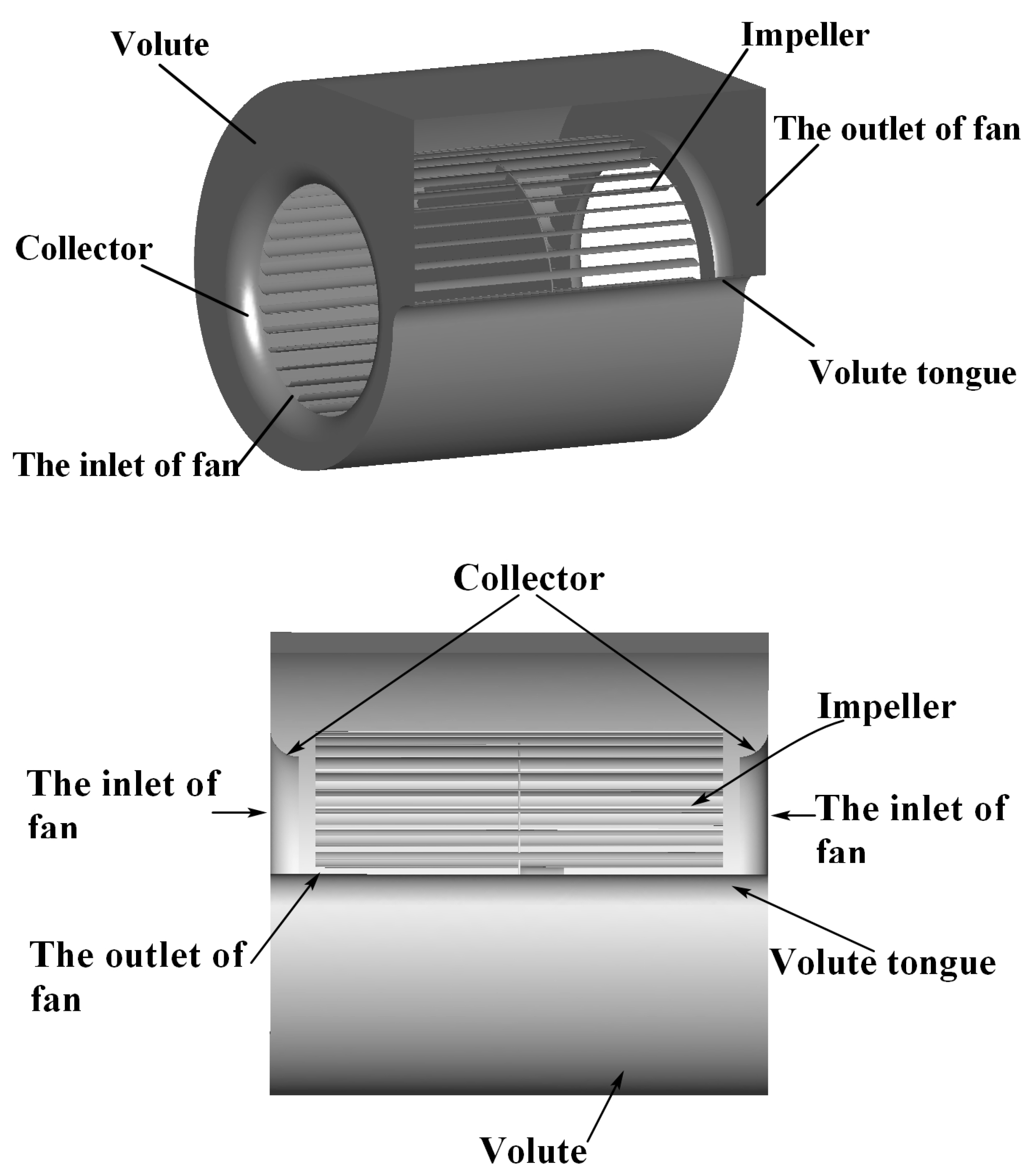
2.1. Centrifugal Fan Model

In general, numerical simulations are an effective tool to study the internal flow laws and unsteady flow characteristics of centrifugal fans. The unsteady numerical analysis is executed on a centrifugal fan with 40 forward wing blades at 1300 RPM. The centrifugal fan is composed by one impeller, a volute, an exit, and two entrances. The volume flow rate of the design point (Q_n) is 321.6 m³/h. The geometric parameters of the model are shown in

Table 1. Design dimensions for the centrifugal fan.

Parameter	Dimension
Impeller inlet diameter (D1)	131.6 mm
Impeller outlet diameter (D2)	150 mm
Impeller width (b)	186 mm
Blade arc radius (Rk)	8.95 mm
Blade thickness (δ)	0.45 mm
Volute width (B)	227.5 mm
Impeller-tongue distance (△t)	11.26 mm
Blade inlet angle (β1A)	84.83°
Blade outlet angle (β2A)	152.04°
Number of blades (Z)	40

, and the structure of the model is shown in Figure 1. In our numerical simulations, the aerodynamic performance and efficiency characteristic curves are obtained by implementing the Renormalization Group RNG k-ε turbulence of steady state, and the unsteady flows are used to study the pressure fluctuation and energy spectrum in a centrifugal fan by implementing the large eddy simulation.

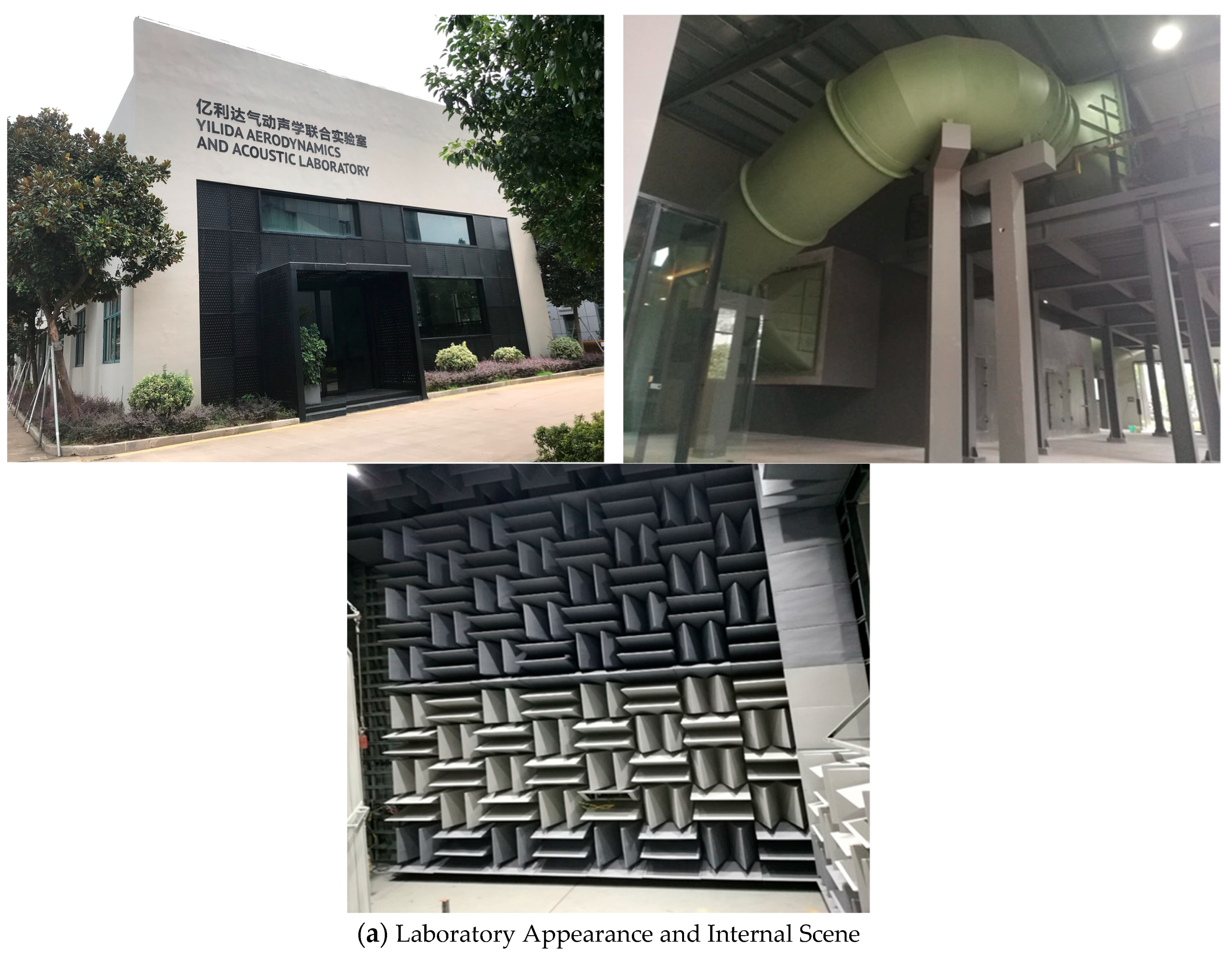
2.2. Laboratory Testing

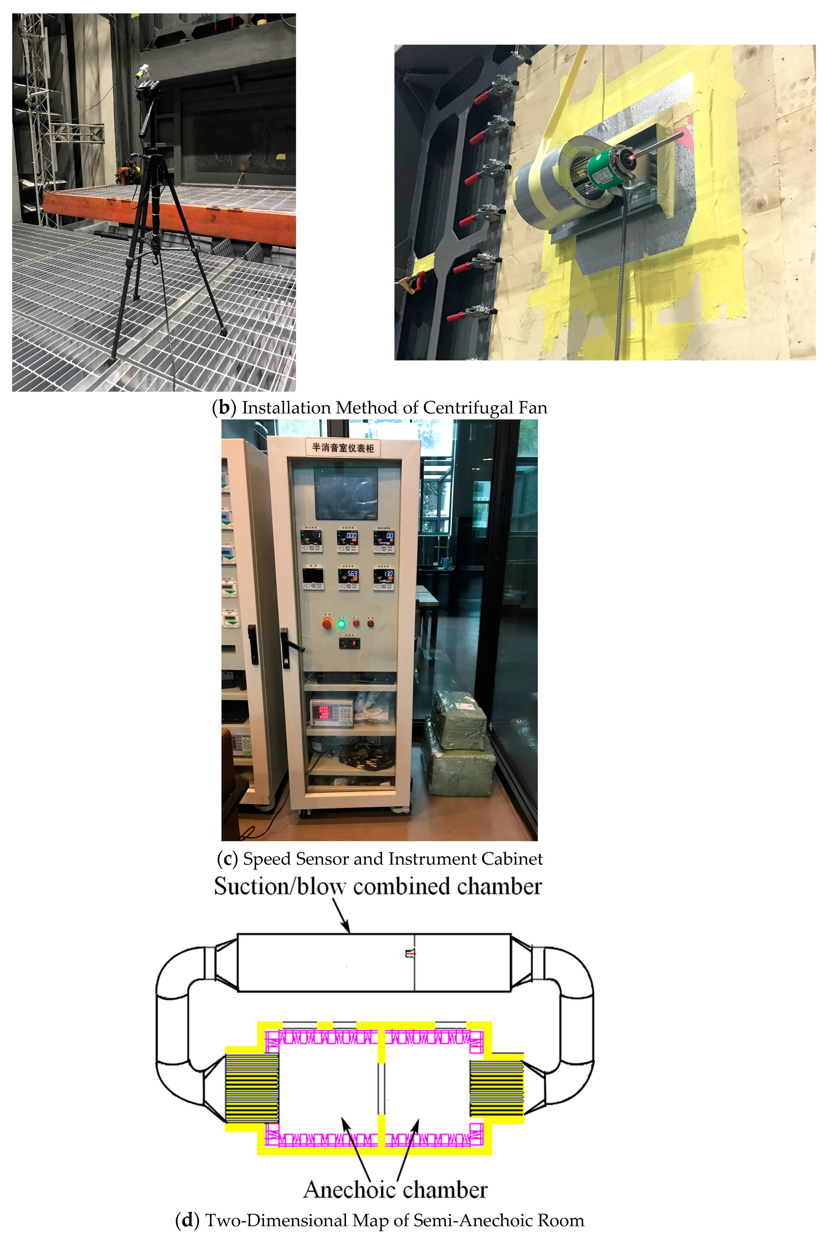
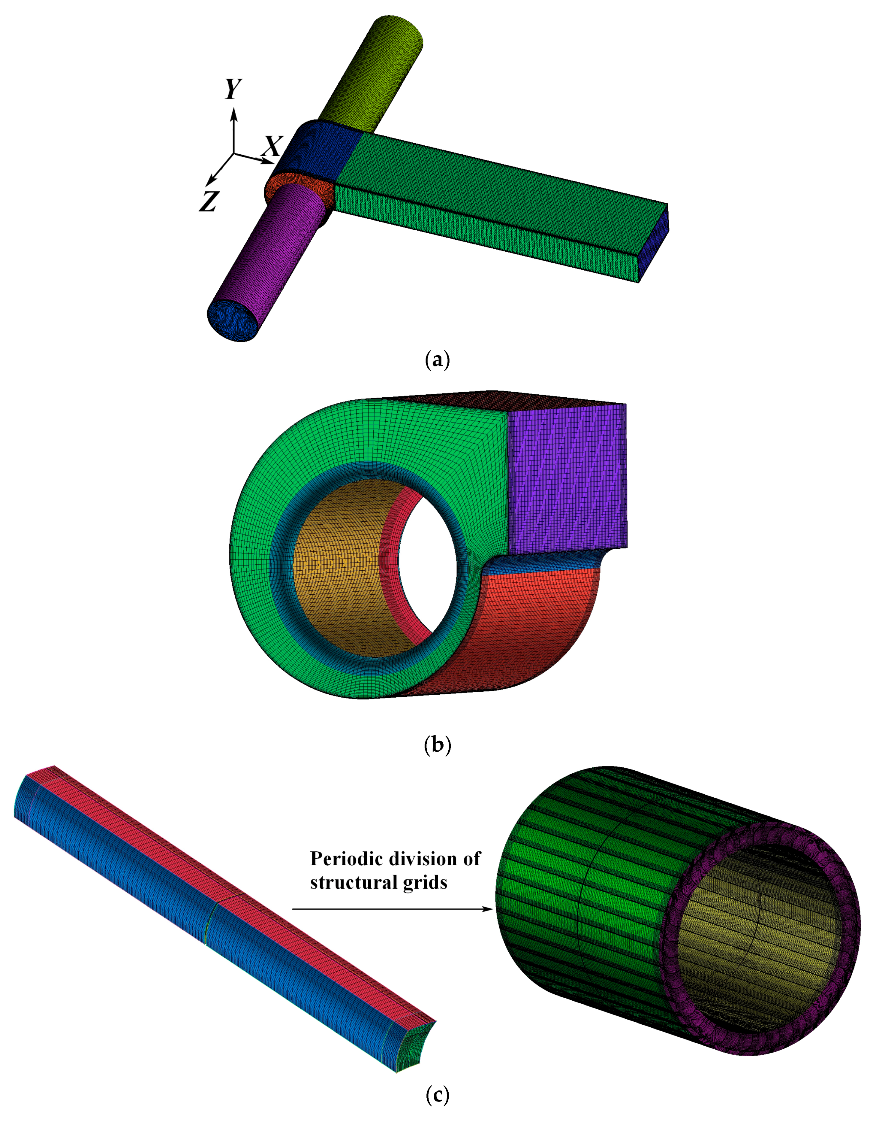
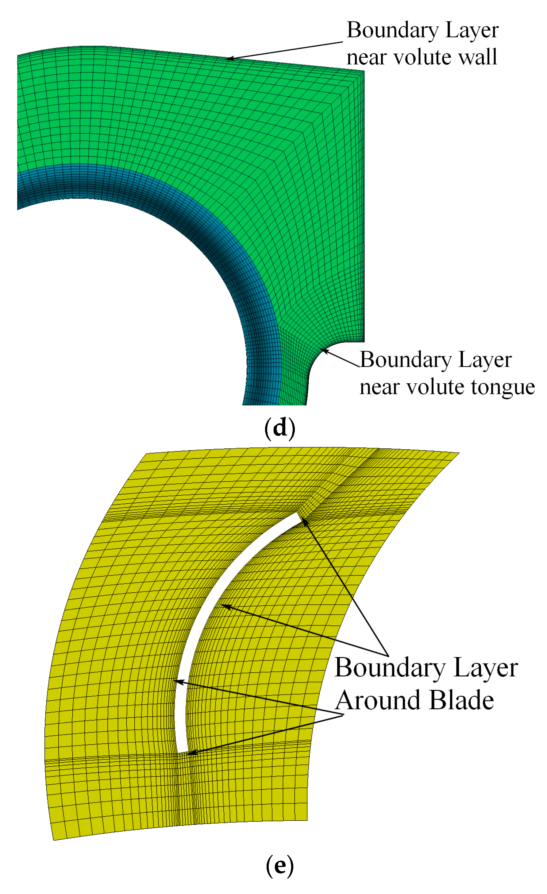
This performance experiment of the centrifugal fan was tested in the Zhejiang Yilida aerodynamics and acoustic laboratory. Figure 2 shows the exterior and interior of the semi-anechoic room in the laboratory. The performance and noise data of a centrifugal fan in a semi-anechoic room can be tested synchronously. The installation method of a centrifugal fan and instrument are also shown in Figure 2.

2.3. Grid System

In our numerical simulations, the centrifugal fan model is supposed to be generated mesh at first. Common grids are divided into unstructured grids and structured grids in Figure 3. Generally, compared with unstructured grids, a structured grid has a fewer number of and more uniform distribution of grid nodes. As is known to all, a large eddy simulation requires more accurate grids in the numerical simulations of centrifugal fans. In order to obtain more precise calculation data, structural grids are adopted in all fluid regions of centrifugal fans. Figure 3b,c show the distribution of structural grids in the impeller domain, respectively. The grid details of the volute are shown in Figure 3d. The flow of fluid on a solid wall will produce a velocity gradient that is perpendicular to the wall direction; accordingly, the grid near the wall needs to be refined, and the details of the mesh near the blade are shown in Figure 3e.

A numerical simulation based on the finite-volume numerical method using FLUENT 16.0 software was carried out to analyze the internal flow of the centrifugal fan at steady and unsteady computations, respectively. All numerical calculations were carried out using a DELL computer including two CPU (2.30 GHz). In order to achieve the verification of grid independence in numerical simulations, four different grid number models, 4.1[M], 4.7[M], 5.4[M], and 6.2[M] were implemented at standard working condition, respectively. Figure 4 shows the static pressure for different numbers of grids. As shown in Figure 4, we can clearly see that the change rate of static pressure is less than 1% at different mesh numbers. Thus, we can ignore the static pressure change. The calculation results are not affected by the number of grids. In the following numerical simulations of the forward multi-wing centrifugal fan, the number of girds in each fluid region and the total grid number are shown in

Table 2. Number of grids in each fluid region of the centrifugal fan.

Fluid Region	Number of Grids	Grid Quality (Determinant 2*2*2)
Inlet (left)	265,933	A range from 0.735 to 0.996
Inlet (right)	293,210	A range from 0.655 to 0.997
Impeller	4,168,320	A range from 0.875 to 0.997
Volute	417,540	A range from 0.612 to 0.999
Outlet	302,621	A range from 0.95 to 1
Total	5,447,624

.

2.4. Steady State Simulation Method

The steady internal flow in a centrifugal fan is studied by implementing the Reynolds-averaged Navier–Stokes Equations method (RANS). As a general rule, the RANS model solves the average information of the flow field. The unsteady turbulence problem is transformed into a steady one, which is sufficient to study the aerodynamic performance of centrifugal fans.

The RNG k-ε was mainly used for the steady calculations in this paper. The e equation in the RNG turbulence model improves the ability to simulate high strain flow. The RNG turbulence model takes turbulent vortices into account, improves the accuracy in this respect, and provides an analytical formula considering the viscous flow of Landmine Nobel Number. This makes the RNG turbulence model more accurate and reliable, so that a swirling flow with moderate intensity and low Reynolds number flow will be well predicted.

The governing equation for a steady flow calculation of the internal flow field of a centrifugal fan is as follows [16,17]:

$$\frac{\partial \left(\rho u_i\right)}{\partial x_i}=0$$

(1)

$$\frac{\partial \left(\rho u_j{u}_i\right)}{\partial x_j}=f_i-\frac{\partial P^{\ast }}{\partial x_i}+\frac{\partial \left[{\mu }_e\left(\frac{\partial u_i}{\partial x_j}+\frac{\partial u_j}{\partial x_i}\right)\right]}{\partial x_j}$$

(2)

where ρ denotes the fluid density; x_i and x_j represent the components x, y, z, u_i, and u_j in the three-dimensional coordinate system; u, v, w, and P* denote the average relative velocity components; fi denotes the component of volume force; μ_ε denotes the coefficient of viscosity; μ_ε = μ + μ_t; μ denotes the molecular viscous coefficient, and μ_t is the viscous coefficient of the turbulent eddy.

$${\mu }_t=\rho C_{\mu }\frac{k^2}{\epsilon }(C_{\mu }=0.0845)$$

(3)

The equation of turbulent energy and the RNG k-ε turbulence model diffusion equation is given as:

$$\frac{\partial }{\partial t}\left(\rho k\right)+\frac{\partial }{\partial x_i}{\left(\rho k{u}_i\right)}_k=\frac{\partial }{\partial x_j}\left({\alpha }_k{\mu }_{eff}\frac{\partial k}{\partial x_j}\right)+G_k+G_b-\rho \epsilon -Y_M+S_k$$

(4)

$$\frac{\partial }{\partial t}\left(\rho \epsilon \right)+\frac{\partial }{\partial x_i}\left(\rho \epsilon u_i\right)=\frac{\partial }{\partial x_j}\left({\alpha }_{\epsilon }{\mu }_{eff}\frac{\partial \epsilon }{\partial x_j}\right)+C_{1\epsilon }\frac{\epsilon }{k}\left(G_k+G_{3\epsilon }{G}_b\right)-C_{2\epsilon }\rho \frac{{\epsilon }^2}{k}-R_{\epsilon }+S_{\epsilon }$$

(5)

where G_k is the turbulent energy due to the laminar velocity gradient, and G_b denotes the turbulent energy g due to buoyancy. C_1ε, C_2ε, and C_3ε denote constants. α_k and α_ε are the Prandtl numbers of the turbulent equation, respectively.

2.5. Transient Simulation Method

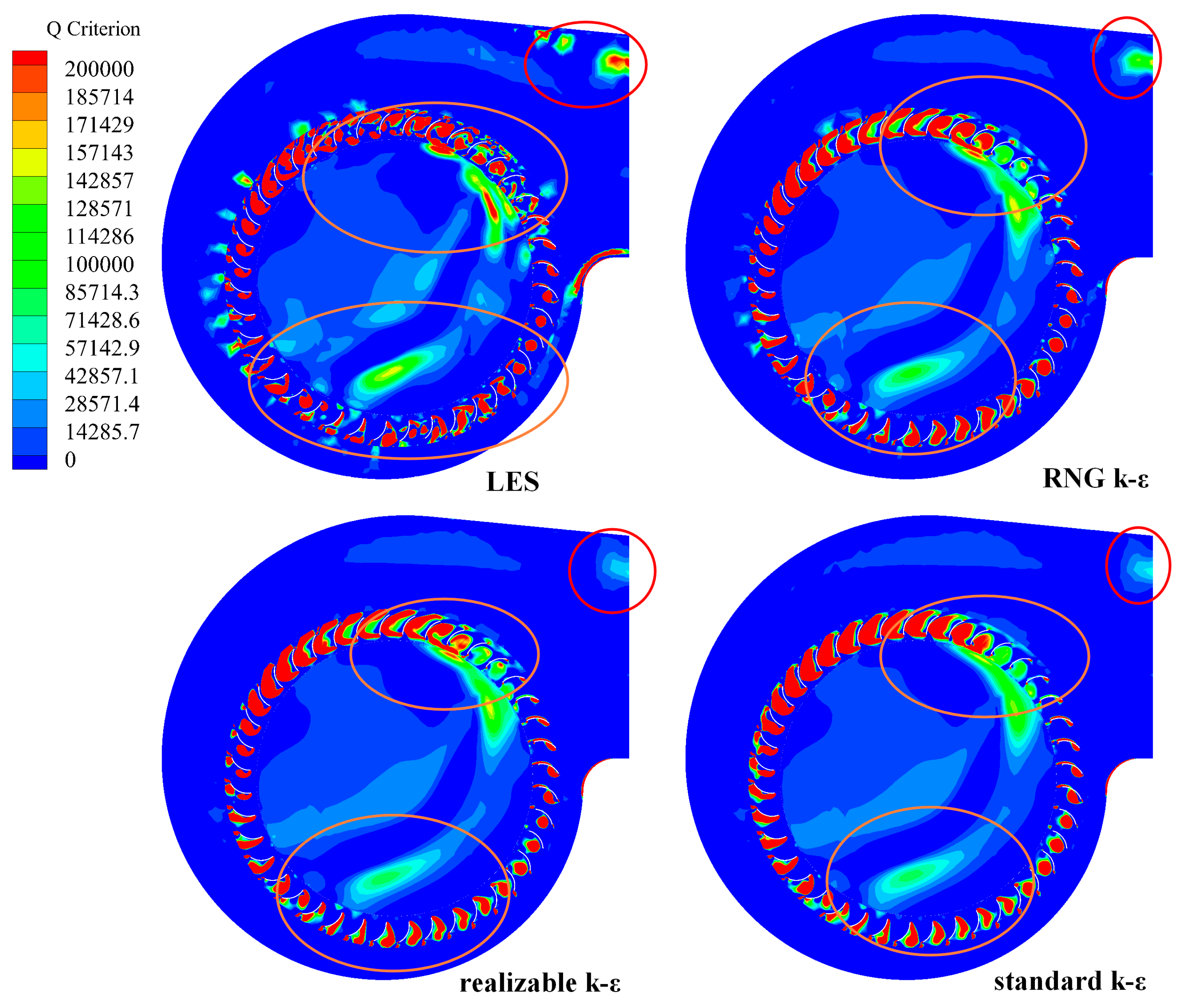
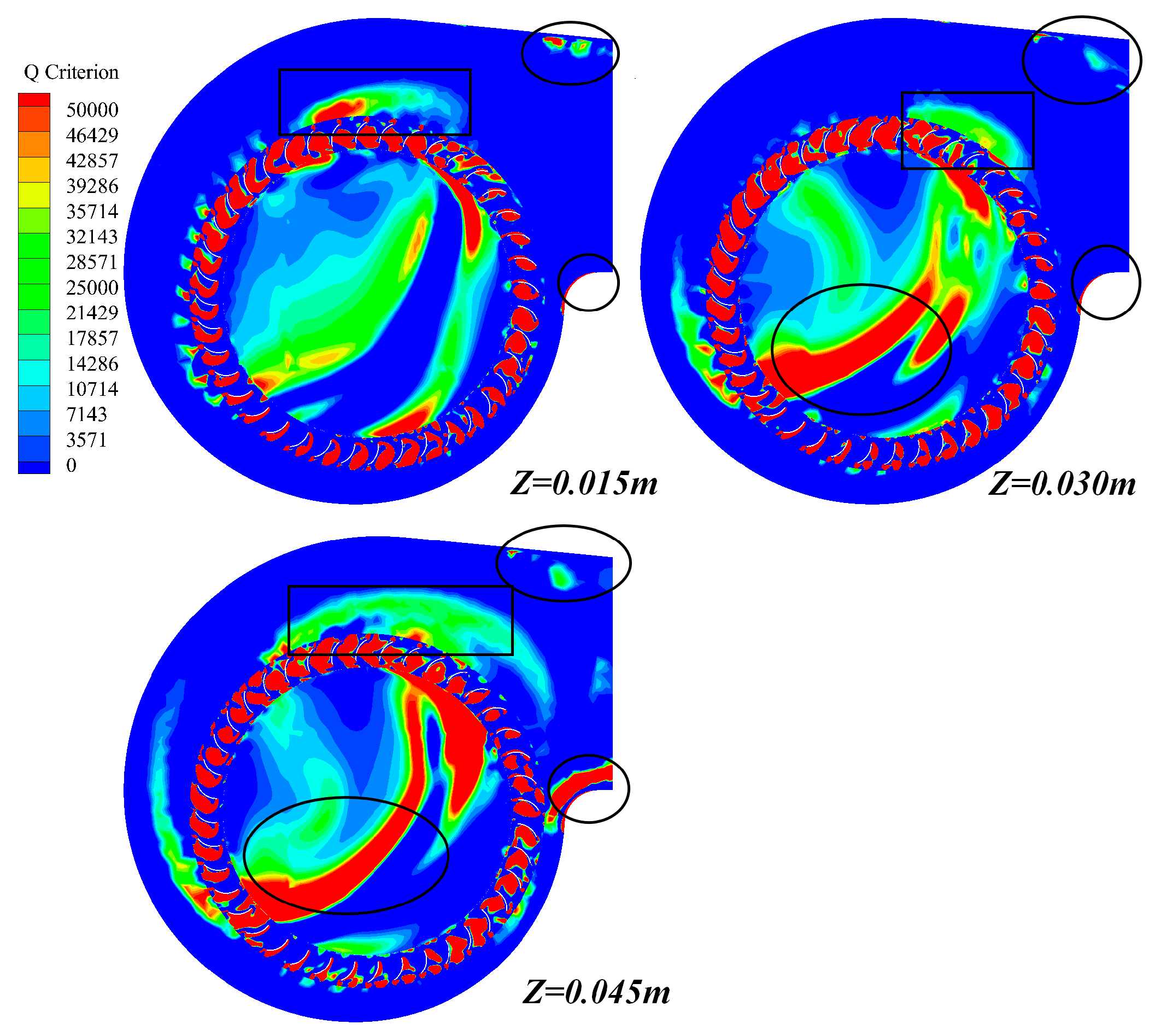
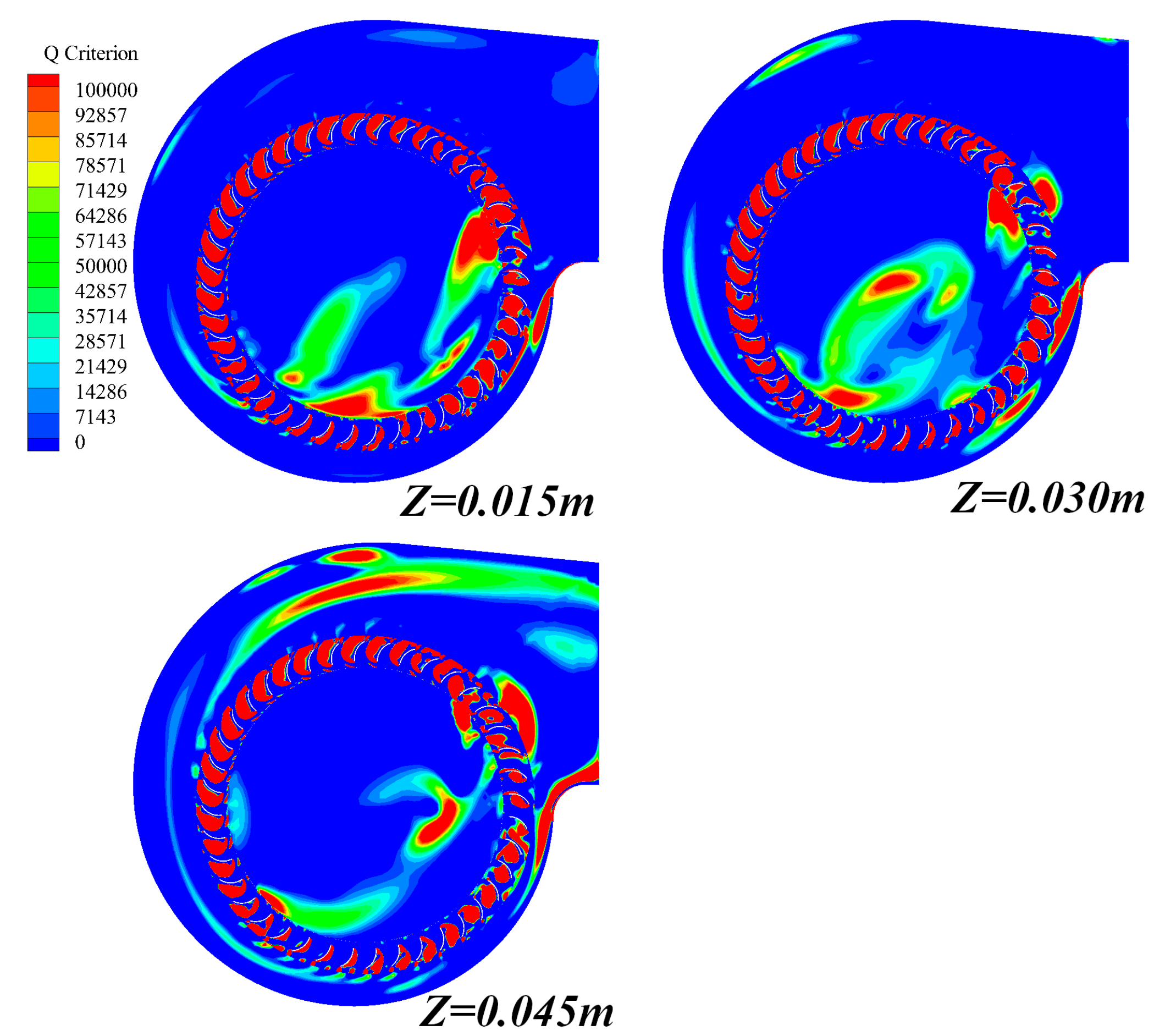
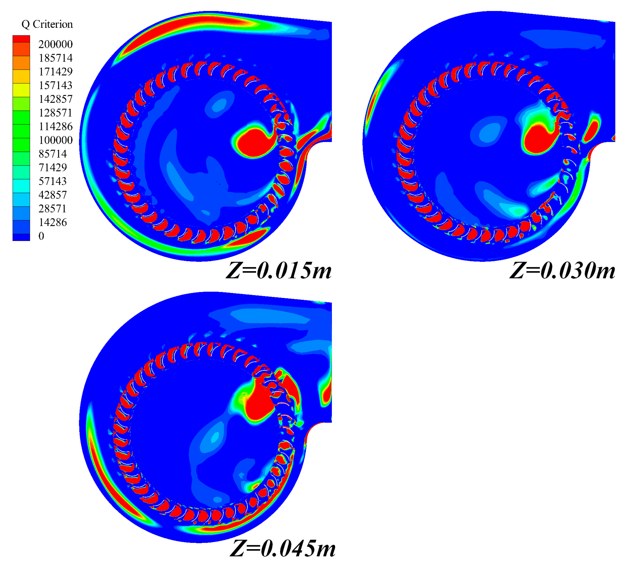
The RANS model is usually used to calculate the time-averaged flow field. The RANS model essentially changes the actual problem, abandons the simulation of unsteady turbulence information, and only seeks the flow results in the average time [18,19,20,21,22]. Hence, it is impossible to simulate unsteady turbulent flow accurately. Nevertheless, the large eddy simulation is a turbulent model to simulate unsteady flow. It solves the instantaneous information of the flow field. The unsteady numerical calculations of the centrifugal fan are also carried out using Large Eddy Simulation (LES), RNG k-ε, realizable k-ε, and standard k-ε models in view of same mesh system at a flow rate of Q/Q_n = 0.031. The same time step was adopted for all the unsteady simulations, and the results at the same time were also analyzed. The difference of Q value distribution is revealed at the Z = 0.015 m plane in Figure 5. The LES model clearly shows more details of the internal vortex structure. On the contrary, the numerical results calculated by the RANS models have limitations on small-scale vortices. The LES model is very useful for most studies of unsteady flow phenomena. Since the small vortices are easily dissipated in the calculation process, the accuracy of the simulation can be improved by using the model instead of the small vortices. Therefore, the following explanations of unsteady flow are all based on numerical results using the LES model.

The basic aim of LES is that turbulence is composed of many eddies of various scales. A large-size vortex has a great influence on the average flow, while a small-size vortex plays a major role in dissipation [11]. Therefore, the mainstream energy in LES is divided into a large-scale vortex and small-scale vortex by some filtering method. A large-scale vortex is directly solved by the Navier-Stokes (N–S) equation, while a small-scale vortex is calculated by establishing the relationship with a large-scale vortex through a sub-grid scale model [23,24,25,26,27,28]. The LES equation can be obtained by filtering the time term from the N–S equation in the Fourier equation or the spatial domain, which can effectively filter out the smaller eddies in the filter mesh, and thus obtain the momentum equation of the larger eddies.

The filtered variables are defined as:

$$\overline{\varphi }\left(\mathrm{X}\right)={\displaystyle \int {}_D}\varphi \left({\mathrm{X}}^{\prime }\right)G\left({\mathrm{X},\mathrm{X}}^{\prime }\right)d{\mathrm{X}}^{\prime }$$

(6)

in which D represents the flow field area, and G denotes the function to determine the size of the filter. The box filtration is frequently employed:

$$\overline{\varphi }\left(\mathrm{X}\right)=\frac{1}{V}{\displaystyle \int {}_v}\varphi \left({\mathrm{X}}^{\prime }\right)d{\mathrm{X}}^{\prime }$$

(7)

in which V denotes the computational element volume. The filter function, G(X,X′), is defined as

$$G\left({\mathrm{X},\mathrm{X}}^{\prime }\right)=\{\begin{array}{ll}\frac{1}{V},& {\mathrm{X}}^{\prime }\in \nu \\ 0,& otherwise\end{array}$$

(8)

By filtering the incompressible N–S equation, the following equations are given as [29]:

$$\frac{\partial \rho }{\partial t}+\frac{\partial }{\partial x_i}\left(\rho \overline{u_i}\right)=0$$

(9)

and:

$$\frac{\partial }{\partial t}\left(\rho \overline{u_i}\right)+\frac{\partial }{\partial x_j}\left(\rho \overline{u_i}\overline{u_j}\right)=\frac{\partial }{\partial x_j}\left(\mu \frac{\partial \overline{u_i}}{\partial x_j}\right)-\frac{\partial \overline{p}}{\partial x_i}-\frac{\partial {\tau }_{ij}}{\partial x_j}$$

(10)

Among them, τ_ij denotes the tension of a sub-grid, which is defined by:

$${\tau }_{ij}=\rho \overline{u_i{u}_j}-\rho \overline{u_i}\overline{u_j}$$

(11)

If the sub-grid tension is obtained after filtration, the eddy viscous model equation is used by the following equation [30,31]:

$${\tau }_{ij}-\frac{1}{3}{\tau }_{kk}{\delta }_{ij}=-2{\mu }_t{\overline{S}}_{ij}$$

(12)

in which u_t is the sub-grid turbulent viscous force and $\overline{S}$_ij denotes the tensor spin, which is defined as:

$${\overline{S}}_{ij}=\frac{1}{2}\left(\frac{\partial {\overline{u}}_i}{\partial x_j}+\frac{\partial {\overline{u}}_j}{\partial x_i}\right)$$

(13)

where u_t is obtained using the Samagorin–Lilly model, which is the basis of the sub-grid model. The equation is:

$${\mu }_t=\rho L_s^2\left|\overline{S}\right|$$

(14)

where:

$$\left|\overline{S}\right|\equiv \sqrt{2{\overline{S}}_{ij}{\overline{S}}_{ij}}$$

(15)

where L_s represents the grid hybrid length; its expression is:

$$L_s=\min \left(\kappa d,C_s{V}^{1/3}\right)$$

(16)

in which ĸ is the von Kármán constant, d is the distance to the nearest wall, and V is the volume of the computational element. C_s = 0.1 is currently implemented.

2.6. Q Criterion

In general, the criteria that is used to judge vorticity includes the Q criterion and vorticity criterion. The application of vorticity criterion requires a given threshold, but different flow thresholds may be different, and different thresholds will result in different results. The Q criterion reflects a balance between the rotation and deformation of a fluid cluster in the flow field. Q >0 reflects the dominance of rotation in flow. At the same time, the Q criterion has no threshold selection, which is more objective than the vorticity criterion.

Different vortex structures reflect the flow characteristics of fluids in various computational domains. The Q criterion is regarded as providing significant physical insight into understanding the internal flow law and the local flow loss in the flow field [19,20,21,22]. To better analyze the internal flow of a centrifugal fan, the Q criterion is considered as a rule of discriminating eddy current in this paper.

The formula is given as:

$${{\displaystyle \mathrm{\Omega }}}_{ij}=\frac{1}{2}\left(\frac{\partial {{\displaystyle u}}_i}{\partial {{\displaystyle x}}_j}-\frac{\partial {{\displaystyle u}}_j}{\partial {{\displaystyle x}}_i}\right)$$

(17)

$${{\displaystyle S}}_{ij}=\frac{1}{2}\left(\frac{\partial {{\displaystyle u}}_i}{\partial {{\displaystyle x}}_j}+\frac{\partial {{\displaystyle u}}_j}{\partial {{\displaystyle x}}_i}\right)$$

(18)

$$Q=\frac{1}{2}\left(\Vert {{\displaystyle \mathrm{\Omega }}}^2\Vert -\Vert {{\displaystyle S}}^2\Vert \right)$$

(19)

3. Results and Discussion

In the following sections, the calculation method and numerical verification are presented firstly. Then, the distribution of physical parameters on different planes is analyzed to understand the internal flow of a centrifugal fan. Finally, the unsteady flow characteristics of the centrifugal fan are comprehended by analyzing the variation of the internal flow field with time evolution.

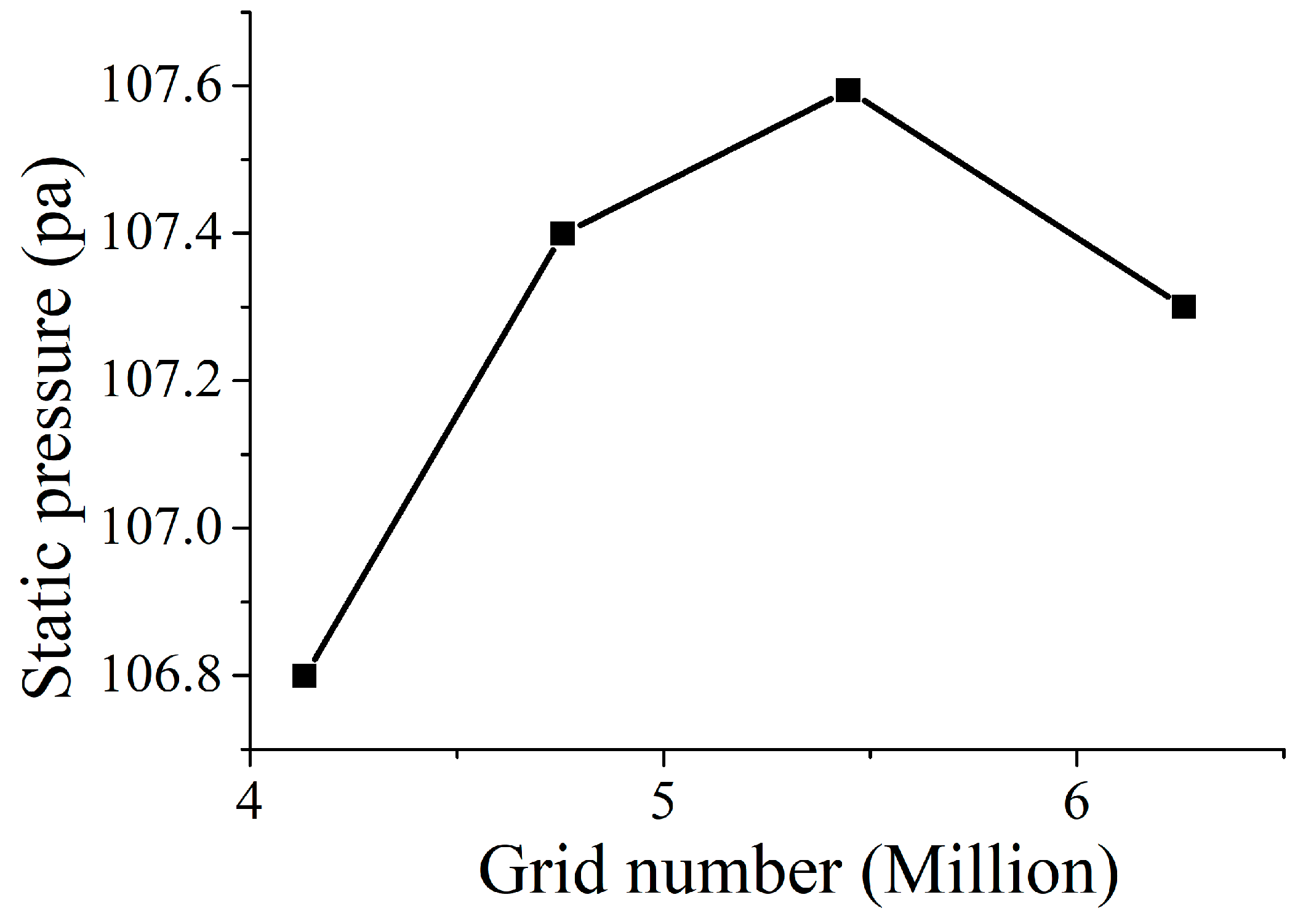
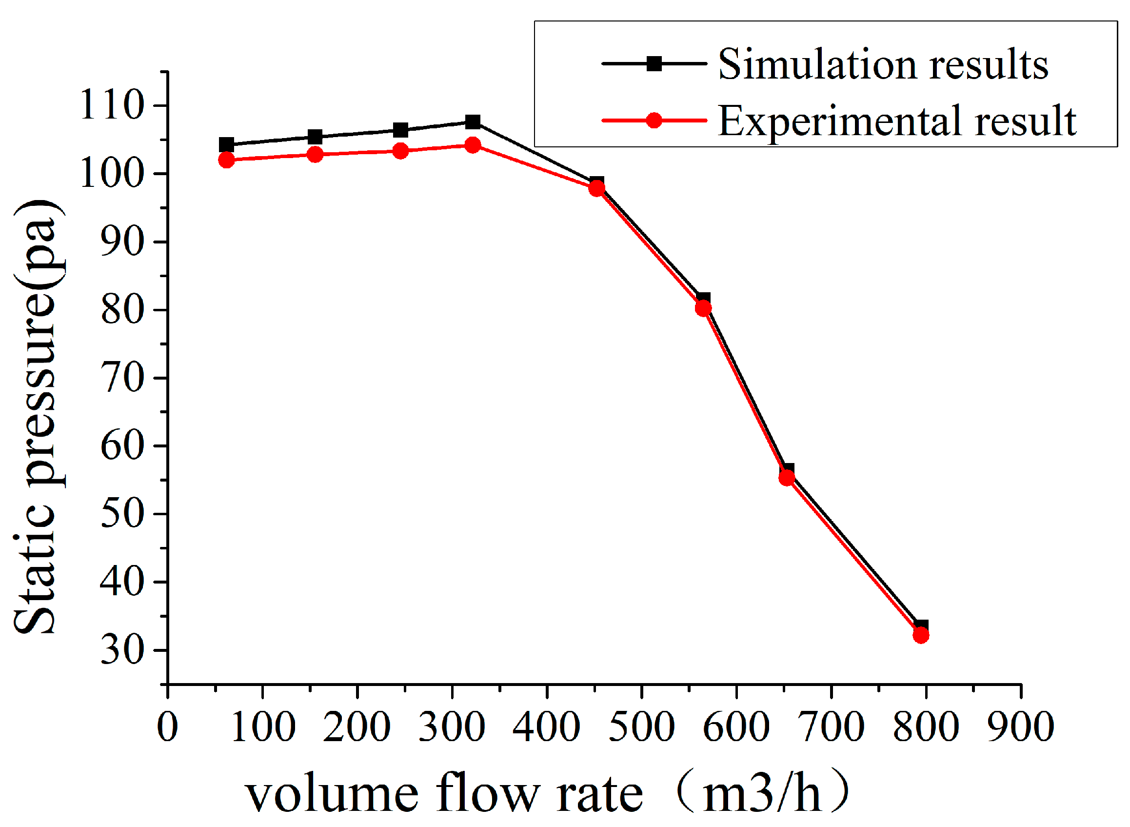
3.1. Numerical Verification

Through steady and unsteady simulations of the centrifugal fan based on computational fluid dynamics (CFD), the internal flow field of the centrifugal fan has attracted a large number of researchers [32,33,34,35,36,37,38,39,40,41,42]. The discrete format at steady calculations is SIMPLE; SIMPLE is also adopted at the unsteady simulations, and the second-order format is carried out in the steady and unsteady simulations. The second-order upwind form is mainly based on a coupled solution of the nonlinear finite difference equations according to the multigrid technique. It is necessary to set a frozen rotor in the steady numerical stimulation, and sliding mesh is applied for unsteady numerical simulation between dynamic and static domains. The time requirement for an impeller to rotate 1 degree 1.25 × 10⁻⁴ s) is considered as the time-step size of unsteady calculation for the sake of more precise detail data. Ten cycles are implemented at the unsteady simulations of the centrifugal fan, so the time steps are 3700.

In order to ensure the correctness and rationality of the calculation results, the forward multi-wing centrifugal fan is tested to acquire the performance data, and is also simulated to obtain calculation data at multiple operating conditions. The static pressure curves of both are shown in Figure 6. As shown in Figure 6, it can be clearly observed that the static pressure obtained by numerical simulations is well consistent with that of the experimental results, which indicates that the numerical simulation method is reasonable in this paper [25,26,27].

3.2. Numerical Results and Discussions of Steady Flow

In this subsection, the static pressure, streamline, and Q value distribution on planes at different positions will be introduced in the internal flow of the centrifugal fan, respectively.

Figure 7 shows the planes of different positions. As shown in Figure 7, the Z = 0 mm plane represents the middle disk, and there are three planes along the positive direction the Z-axis; their locations are Z = 0.015 m, Z = 0.030 m, and Z = 0.045 m, respectively. The parameters on the three planes will be presented by the analysis of the steady results.

Figure 8 exhibits the static pressure distribution of different planes. From Figure 8, it can be seen that the static pressure along the positive direction of the Z-axis presents different static pressure distribution at three locations. The large area of low pressure appears near the blade channel, and the plane low-pressure area at Z = 0.015 is smaller than that of the other two planes. In the volute tongue position and volute outlet position, high hydrostatic pressure distribution and gradient change are observed in all three planes, and the greatest pressure gradient occurs at the Z = 0.030 m plane. It is further indicated that the fluid reflux phenomenon occurs at the high-pressure gradient location of fluid flows from the high static pressure region to the low static pressure region.

Figure 9 expresses the streamline distribution at different planes. As shown in Figure 9, the difference of streamlines in the internal flow of centrifugal fan with the increase of Z-axis distance is clearly observed. The comparison of streamline distribution on different planes indicates that near the impeller entrance, no vortex streamlines occur on the two planes z = 0.015 m and z = 0.030 m, but some small vortex streamlines appear on the plane z = 0.045 m. Most importantly, a large number of small-scale eddies are caused by boundary layer separation on the wall above the volute outlet. It is further found that fluid refluxes obviously occur on the Z = 0.045 m plane and the direction of fluid flow has changed greatly, followed by the Z = 0.015 m plane in the vicinity of the volute outlet, which is well consistent with the distribution of the static pressure in Figure 7.

Figure 10 gives the distribution of Q values at different planes in the internal flow of centrifugal fans. The Q criterion is implemented to analyze the internal flow of centrifugal fans, which is regarded as one of the criteria of judging vortices. The region with a larger Q value represents the phenomenon of vortices. We can see clearly that the distribution of Q values assumes differences at three planes in Figure 6. It is clearly observed that the significant distribution differences of the Q values occur at the marked position of the impeller entrance. The high Q value appears on the Z = 0.045 m plane, the significant distribution differences of the Q values occur at the marked position of the impeller, a slight reduction occurs on the Z = 0.030 m plane at the same position of Z = 0.045 m, and a significant reduction occurs on the Z = 0.015 m plane compared with that of Z = 0.03 m and Z = 0.045 m. In the marked position of the impeller exit, all three planes have higher Q value distribution; however, the area with a high Q value on the Z = 0.045 m plane is obviously larger than that of the other two planes. A small part district of a high Q value appears in the upper part of the volute outlet. At the cochlear volute tongue position, the Q value of the Z = 0.045 m plane is significantly higher than that of the other planes. The different distributions of Q values on the planes represent the flow conditions of different fluids. The Q value shown in Figure 10 coincides with the static pressure in Figure 8 and the streamline in Figure 9.

Figure 11 describes static pressure of cross-sections at different positions at the flow rate Q/Qn = 1. As we can see from Figure 11, the static pressure distribution is slightly different, mainly in the vicinity of the volute tongue. The static pressure distribution is similar on the Z = 0.015 m and Z = 0.030 m planes, but it is very uniform on the z = 0.045 m plane.

Figure 12 exhibits the streamline distribution of different planes. As shown in Figure 11, one can see that the airflow can flow smoothly along the volute outlet, but it is different near the volute tongue. This also reflects that the air flow at the volute tongue is more complex.

Figure 13 shows the Q value distribution of different planes at a flow rate of Q/Qn = 1. It is clearly observed that the Q value distribution in the impeller is not uniform, and the Q value is higher in the upper region of the volute and volute tongue. This corresponds to the streamline chart.

Figure 14 represents that the static pressure of different positions at the flow rate Q/Qn = 1.758. Figure 14 clearly shows that the static pressure distributions of different sections are similar. The static pressure gradient varies greatly, and a higher static pressure appears near the cochlear tongue, which makes the airflow in the cochlear tongue unstable.

Figure 15 shows that streamline of cross-sections at different planes at a flow rate of Q/Qn = 1.758. From Figure 15, it can be seen that there is an eccentric eddy current at the impeller inlet at three positions. Due to the complex flow near the volute tongue, the airflow here is unstable.

Figure 16 shows the Q value distribution of cross-sections at different positions at a flow rate of Q/Qn = 1.758. From Figure 16, it can be seen that there is a large Q value distribution at the impeller entrance, which corresponds to the eccentric vortices in the streamline diagram. A large Q value distribution also appears in the upper part of the volute on the Z = 0.015 m plane.

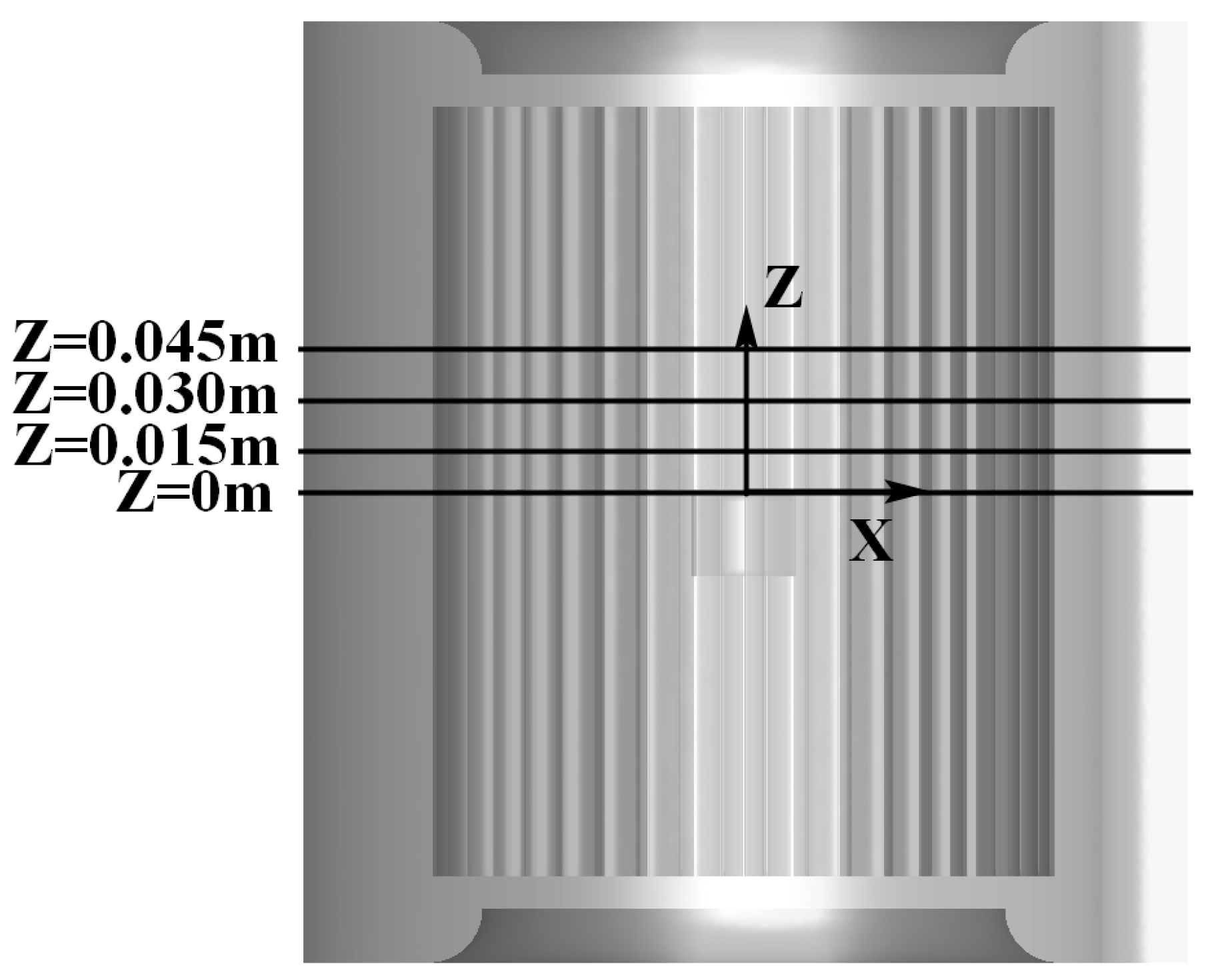
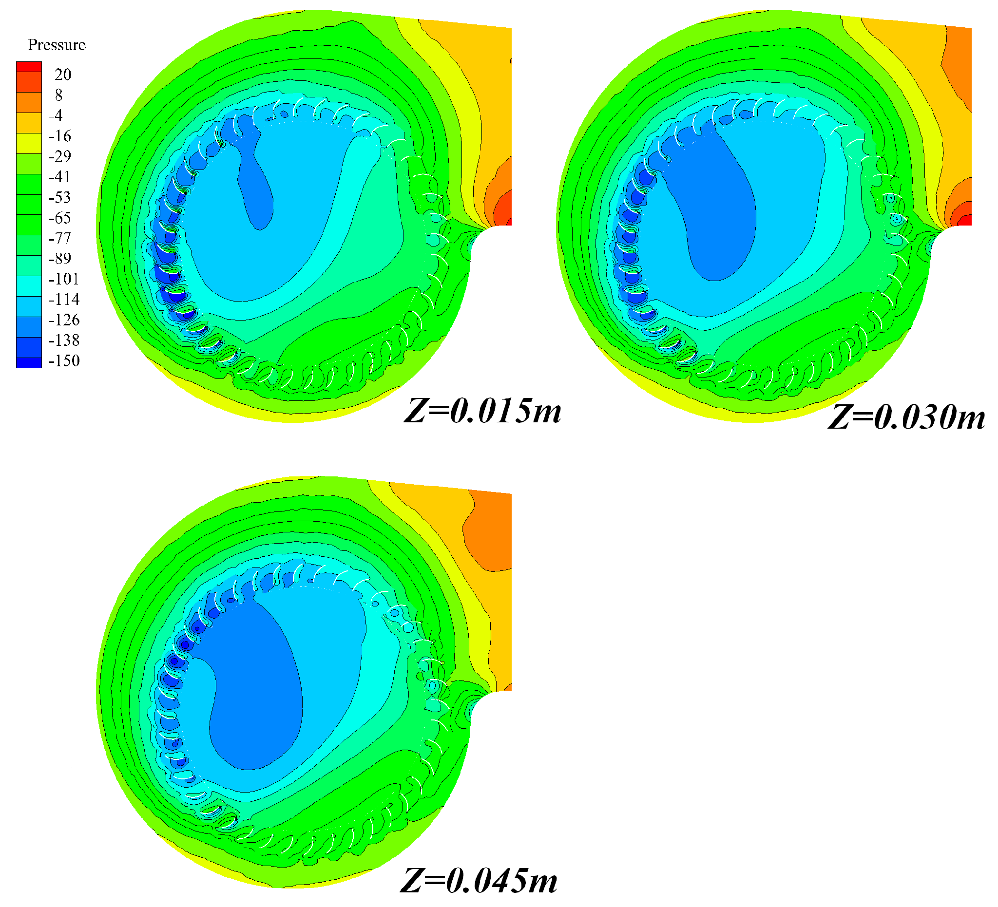
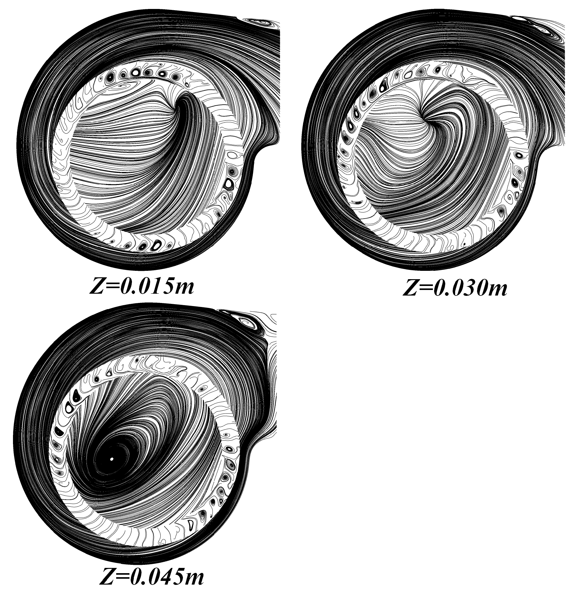
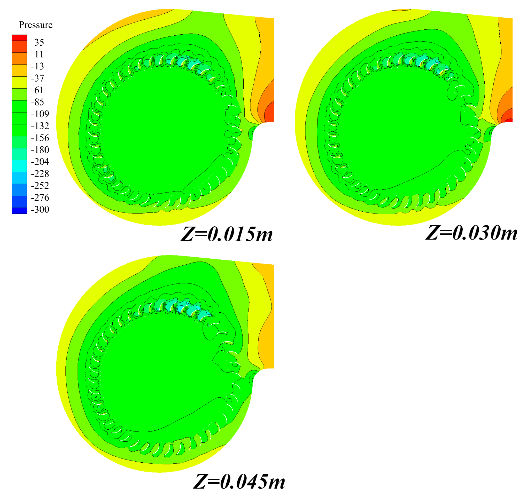
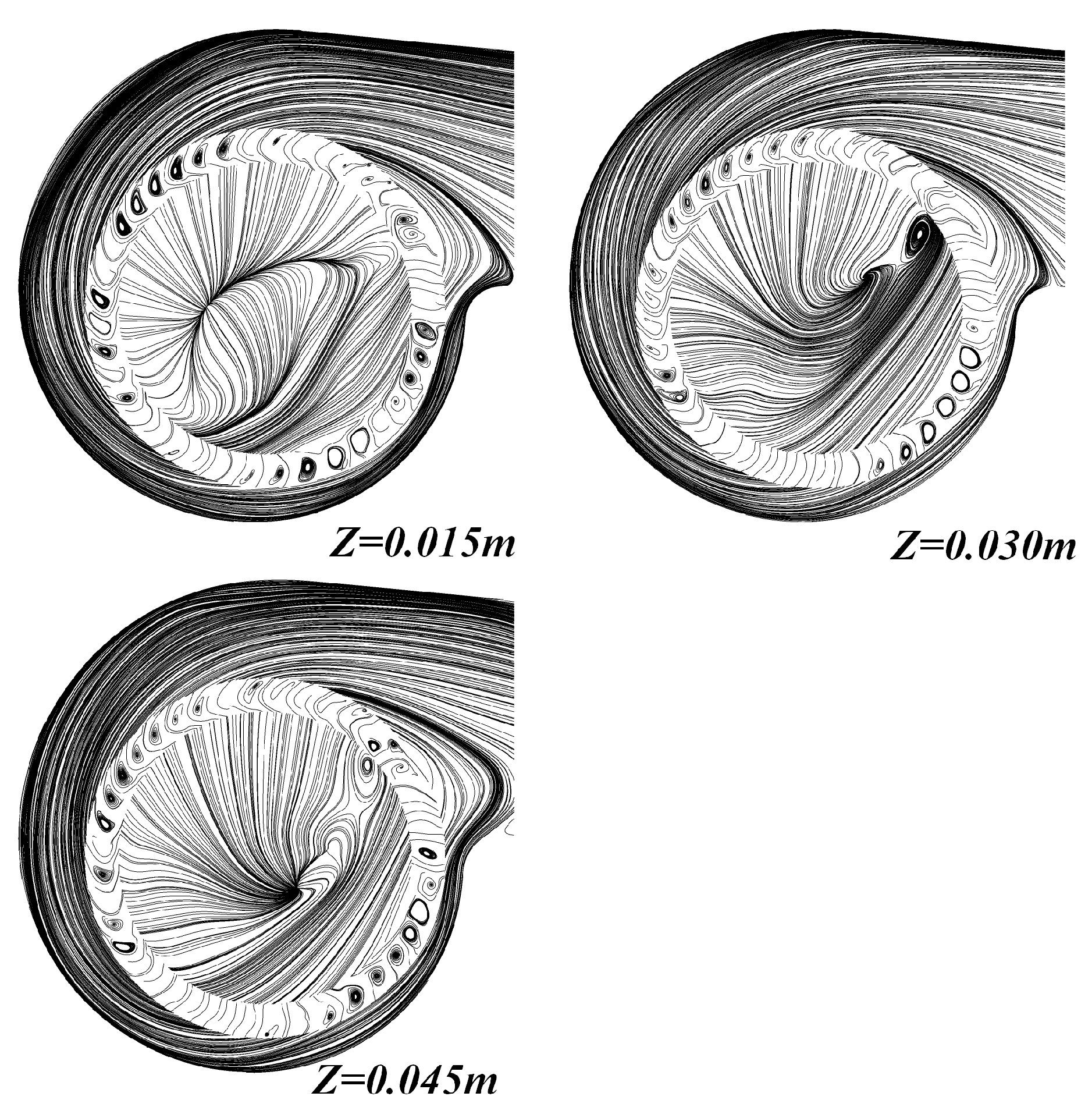
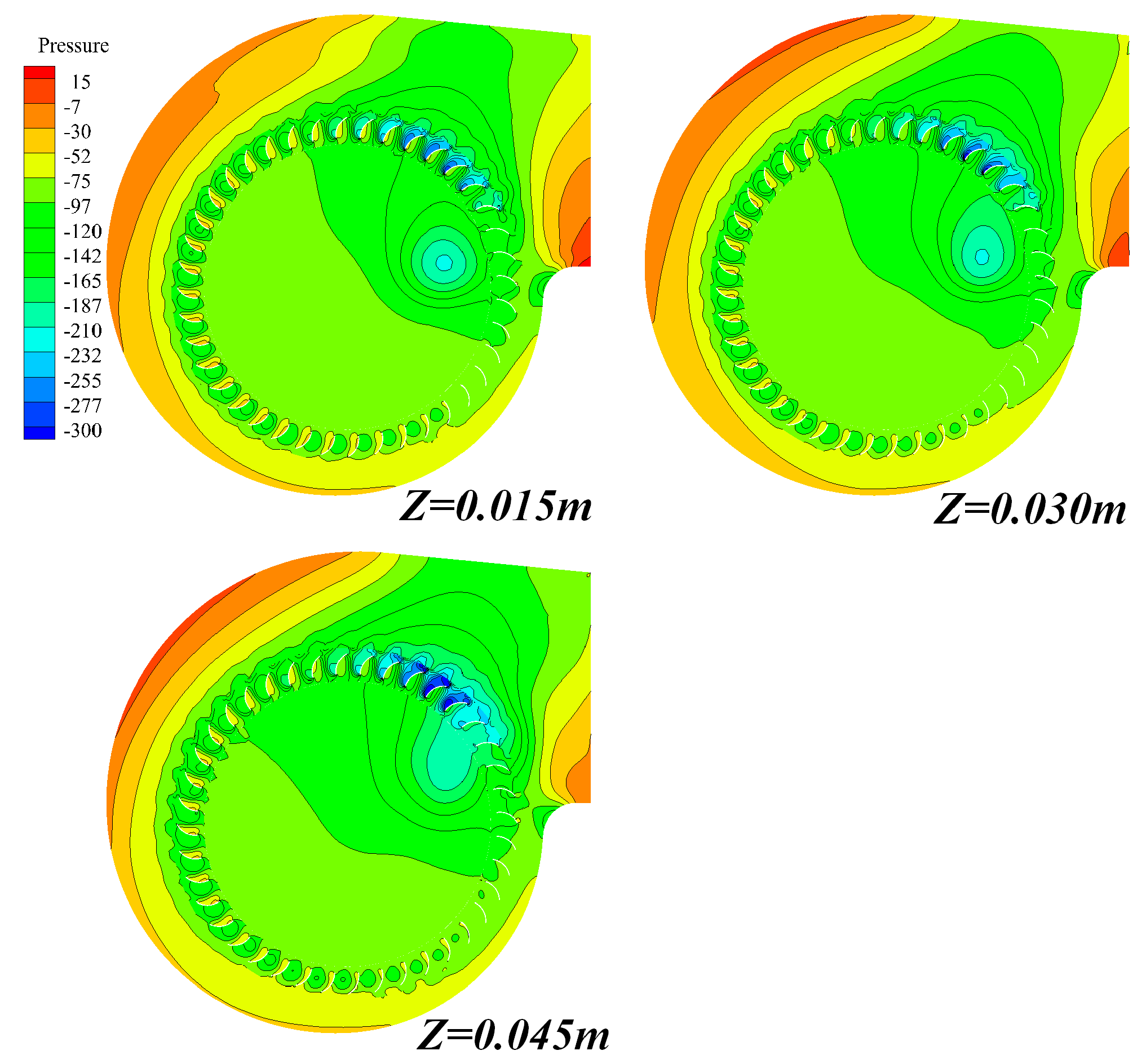
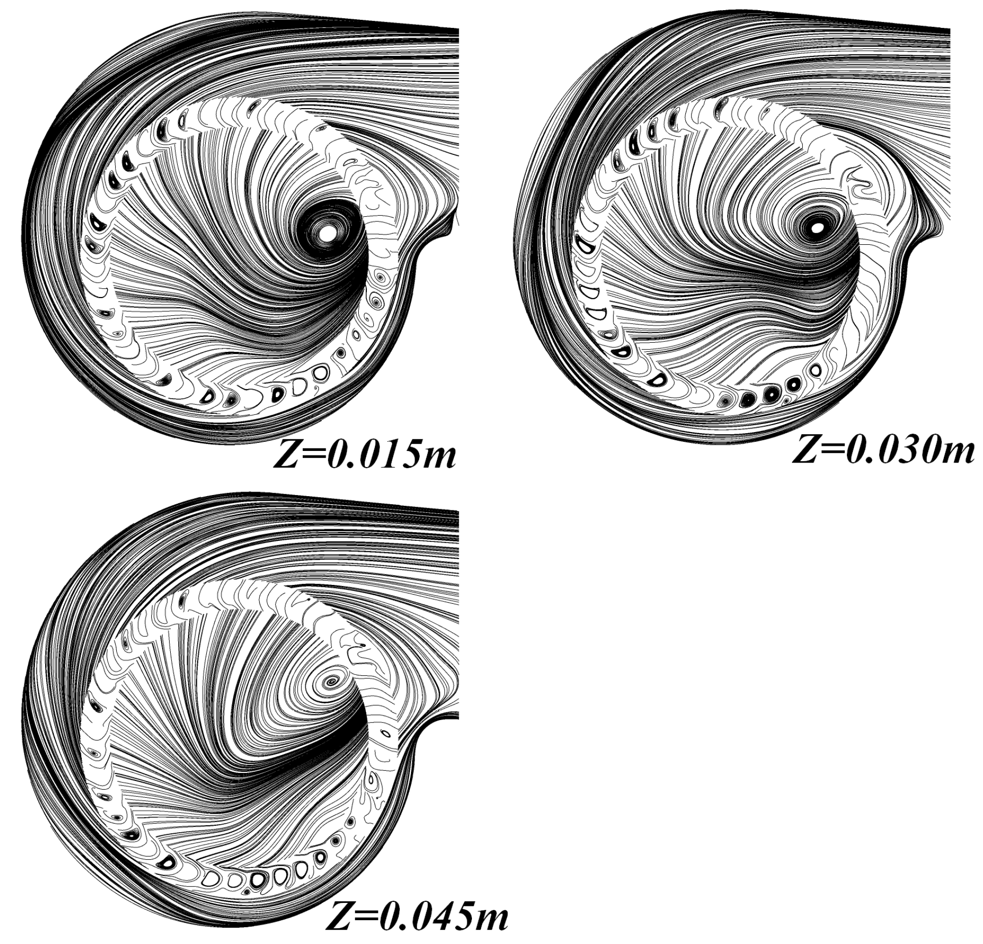
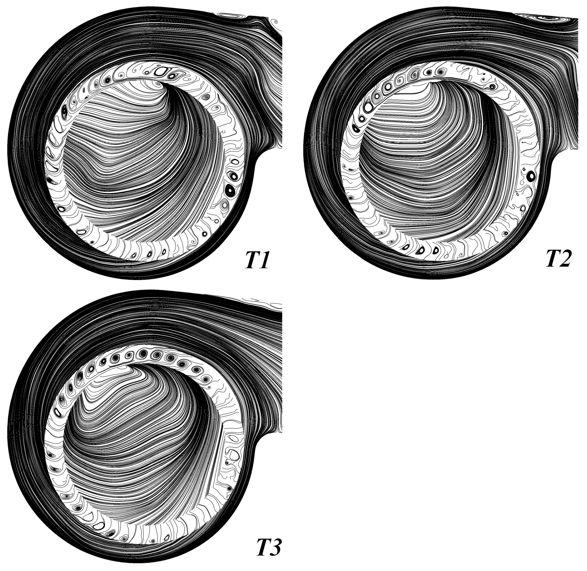
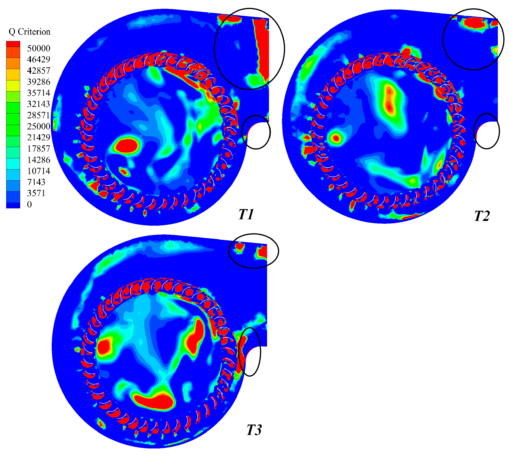
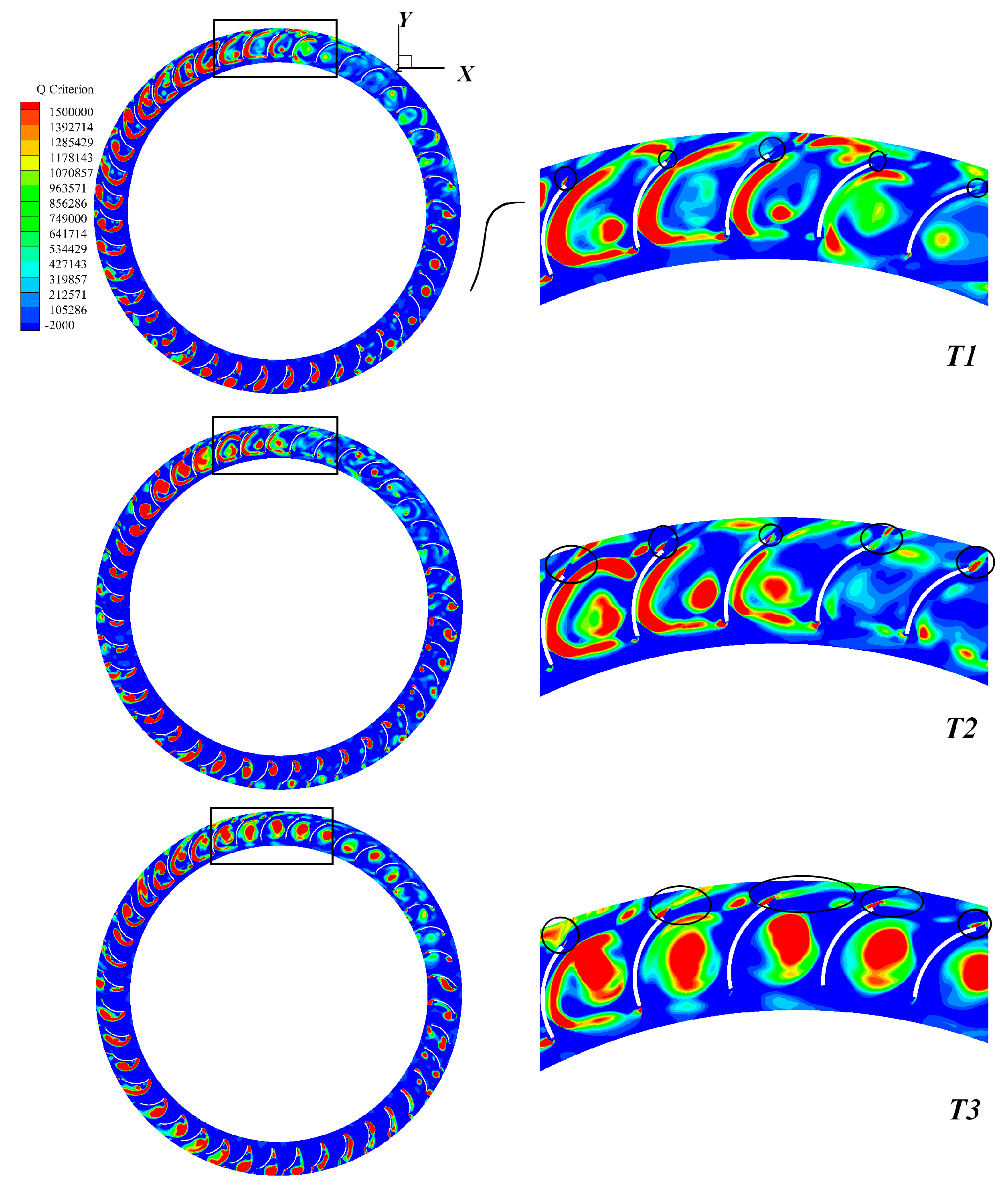
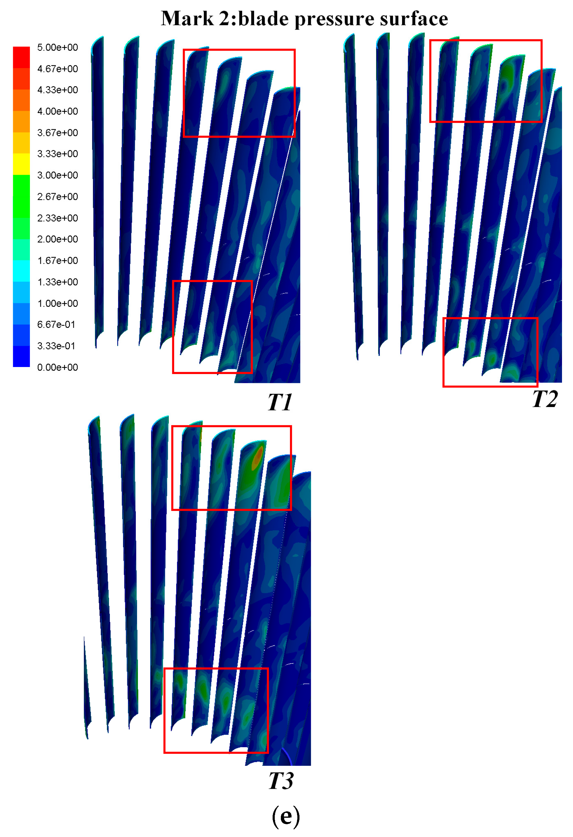
3.3. Unsteady Internal Flow Structure

In this subsection, the static pressure, streamline, and Q value distribution on the Z = 0.015 m plane with time evolution will be introduced in the internal flow of the centrifugal fan. Then, the three-dimensional eddy phenomena of the impeller and volute domains are analyzed at different Q values.

Figure 17 proves the static pressure distribution with time evolution on the Z = 0.015 m plane. Plotted in Figure 17, one can see that the static pressure distribution constantly transforms with time evolution near the impeller inlet and volute outlet. There is a low-pressure area near the impeller entrance, and a little gradient change of the low-pressure area occurs near the impeller entrance with time evolution. The most important part is that the static pressure gradient of the volute tongue and the volute outlet changes greatly; there are two high-pressure areas at the time of T₁, a wide range of high-pressure areas at the time of T₂, and a high-pressure area at the time of T₃ only appears at the cochlear volute tongue position. The most obvious static pressure gradient of the volute tongue appears at the time of T₂; however, the static pressure gradient of the volute at the time of T₃ is evidently decreased.

Figure 18 exhibits the streamline distribution in a centrifugal fan with time evolution at the Z = 0.015 m plane. From Figure 18, we can distinctly observe that streamlines in the middle of a plane do not change much in the course of time lapse, but the streamlines at the volute outlet gradually become smooth, and reflux occurs with time evolution. The phenomenon of boundary layer separation above the volute outlet gradually weakens, which coincides with the static pressure distribution in Figure 16.

Figure 19 displays the distribution of Q values with time evolution on the Z = 0.015 m plane. As shown in Figure 19, it is clearly observed that the distribution of the Q value changes with time evolution appear in the upper part of the volute outlet and near the volute tongue. The Q value above the volute outlet decreases gradually from a high value, and the area diminishes over time evolution. Near the cochlear volute tongue, a higher Q value appears at the time of T₃. This corresponds to the flow phenomena described in Figure 16 and Figure 17.

In order to further explain the internal flow physical essence of a centrifugal fan, the Q value distribution of the blade passage is presented with evolution at different times on the Z = 0.015 m section in Figure 20. As shown in Figure 20, it is clearly seen that the Q value is higher near the suction surface and at the end of the blade. When airflow flows through the blade passage, the flow pattern around the blade is complex. The separate flow appears near the suction surface, and an obvious eddy current exists at the tail of some blades, whereas the flow pattern around the blade wake is disordered. For the local enlarged image, the boundary layer separation occurs near the suction surface in the blade passage, and the Q value is obviously becomes high at T₃. With the impeller rotating, the suction surface airflow separation cluster will fall off at the end of the blade. At the time of T1, the eddy current is not obvious at the end of the blade, and with the fan running, the eddy at the end of the blade will gradually become obvious, and the area will increase. The boundary layer separation on the suction surface and the shedding vortices at the end of the blade will lead to the pulsating reaction in the flow passage of volute.

Figure 21 shows the skin friction coefficients of the pressure surface and suction surface of the blade. The magnitude of the friction coefficient on the blade surface indicates the velocity near the blade surface. If the friction coefficient is positive or negative in a region, which indicates that the direction of local flow is inconsistent, then flow separation or reattachment occurs in the region. As we can see from Figure 21, there is no negative value of friction coefficient on the suction surface or pressure surface of the blade, expressing that no obvious flow separation has occurred. At Mark 1, the friction coefficient is higher, because the rotation of the impeller makes the air accelerate. However, the friction coefficients of the pressure surface and suction surface are similar. At Mark 2, the friction coefficient on the suction surface of the blade changes slightly with time, and a high friction coefficient appears on both ends of the blade at T₂. The variation of the friction coefficient gradient at both ends of the blade makes the local flow unstable. The friction coefficient of the blade pressure surface is smaller than that of the suction surface over time. This indicates that the flow becomes unstable due to the large velocity variation in the blade passage.

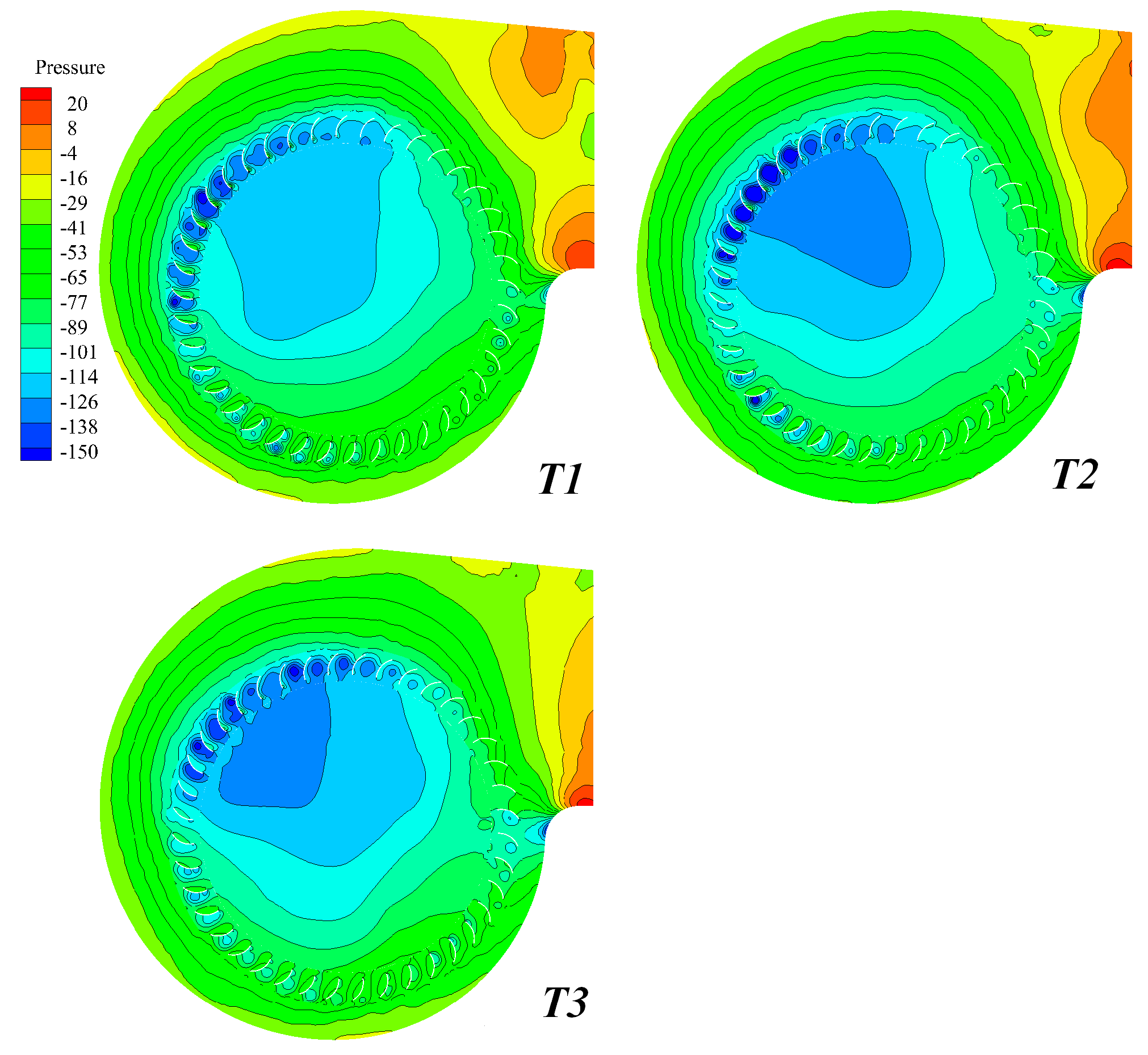
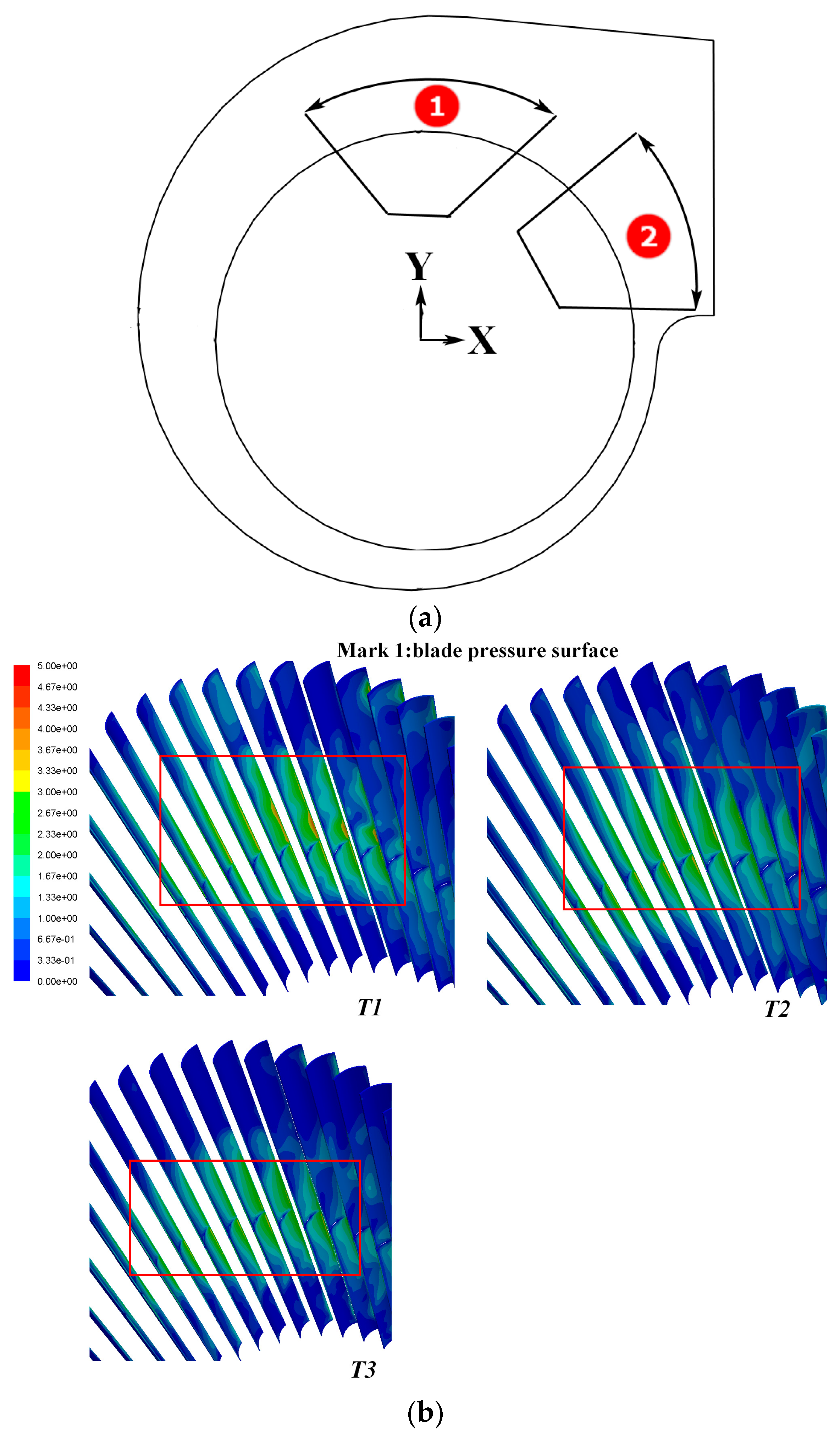
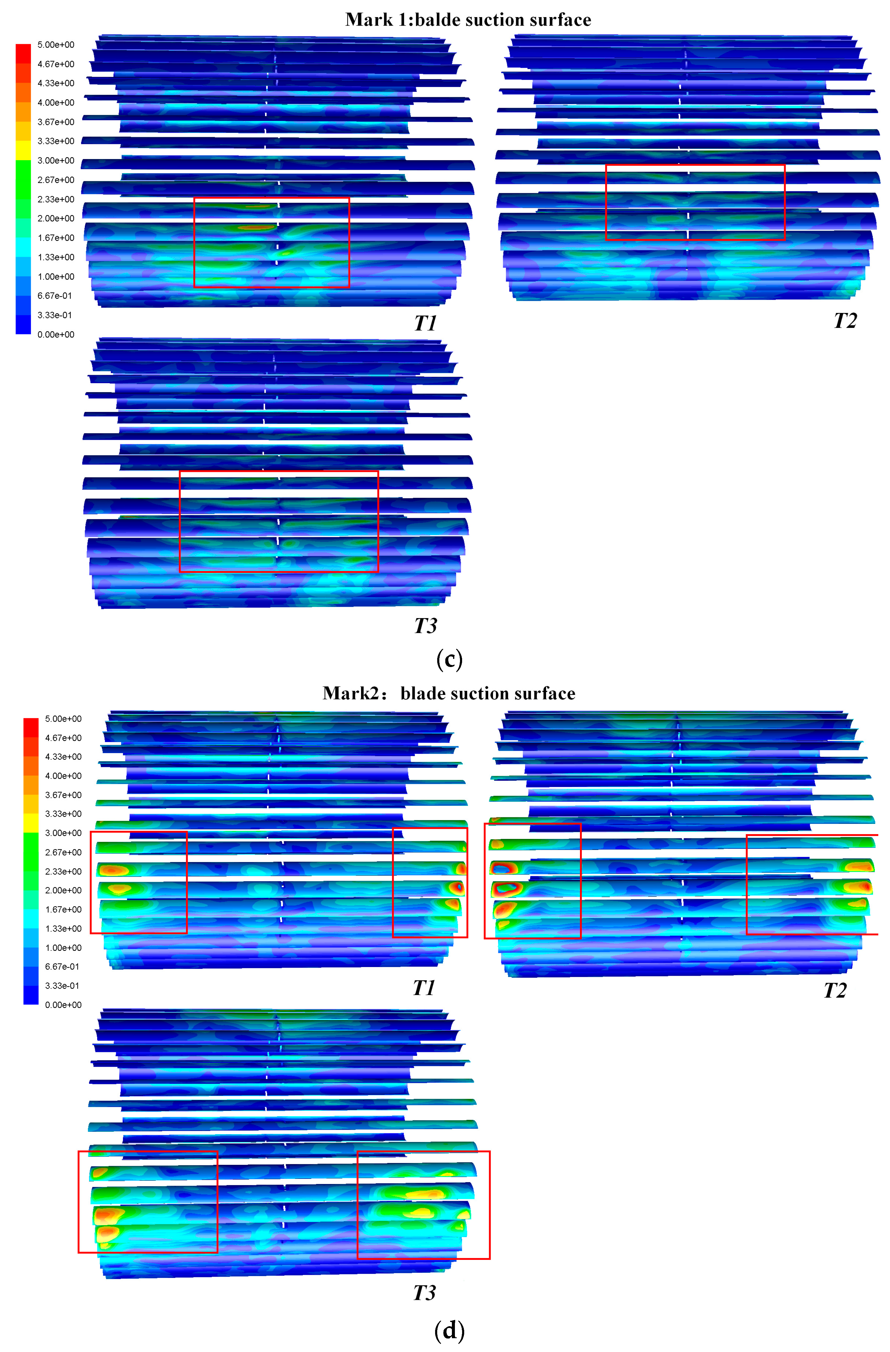
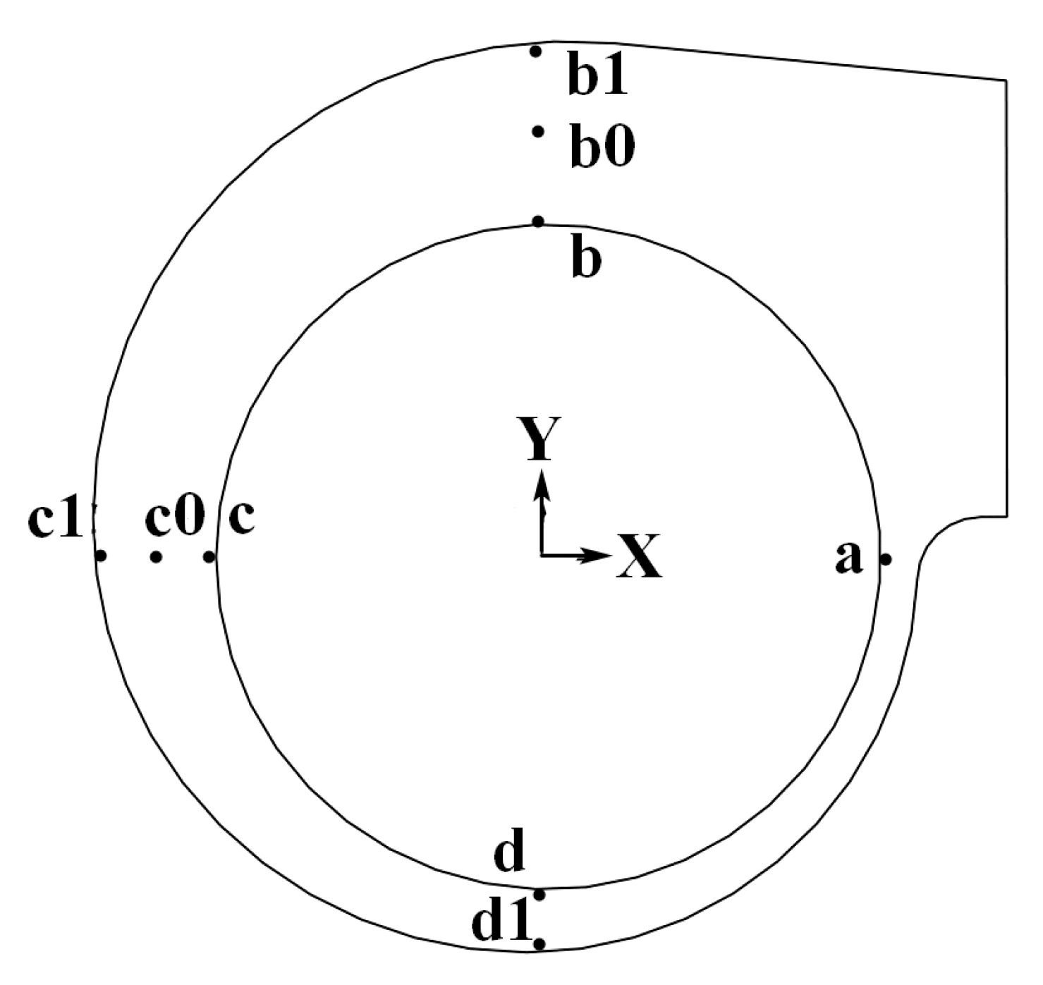
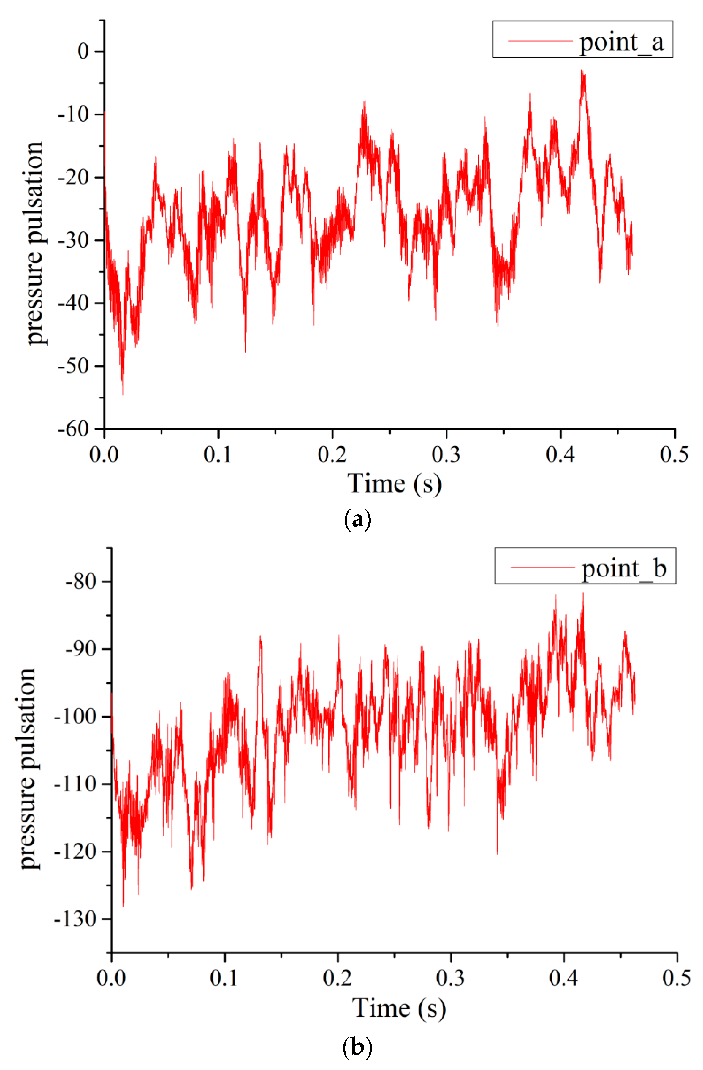
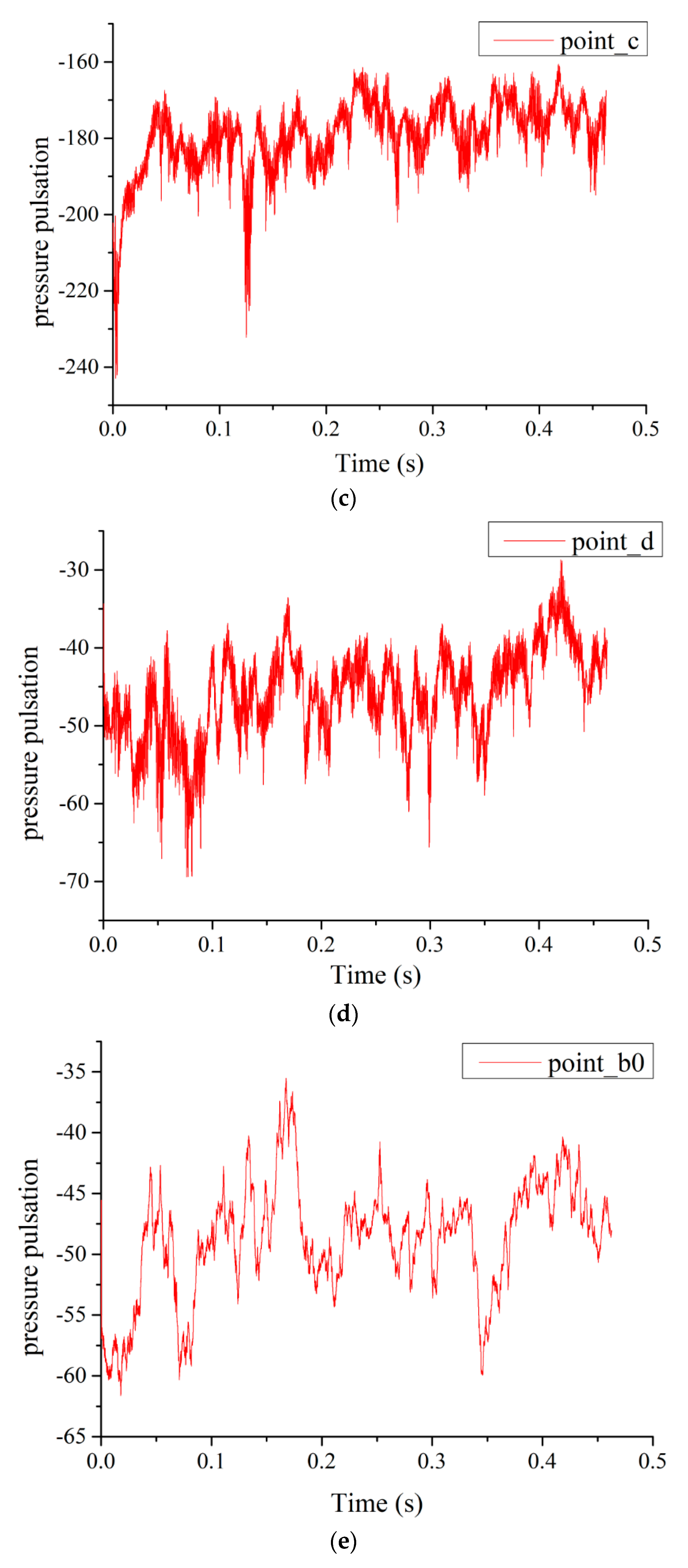
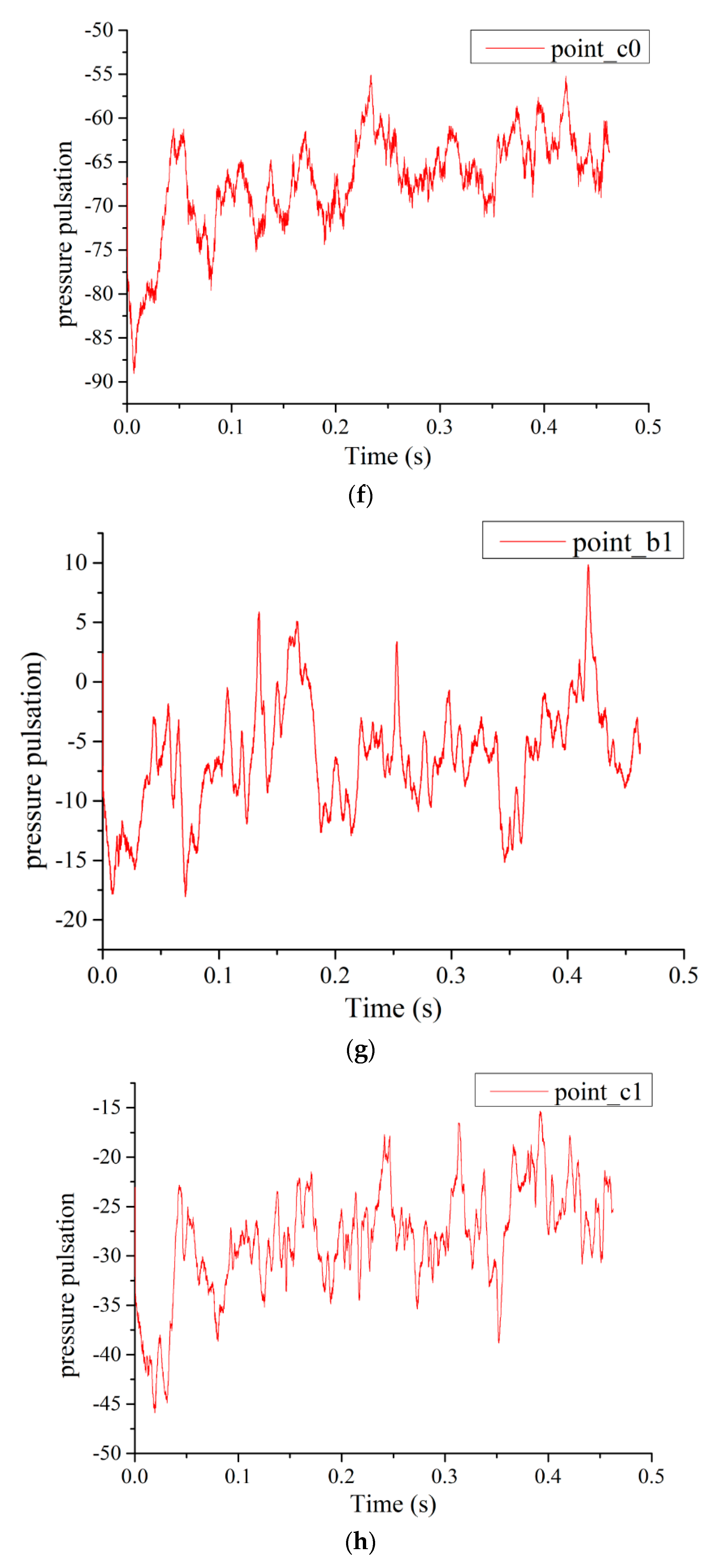
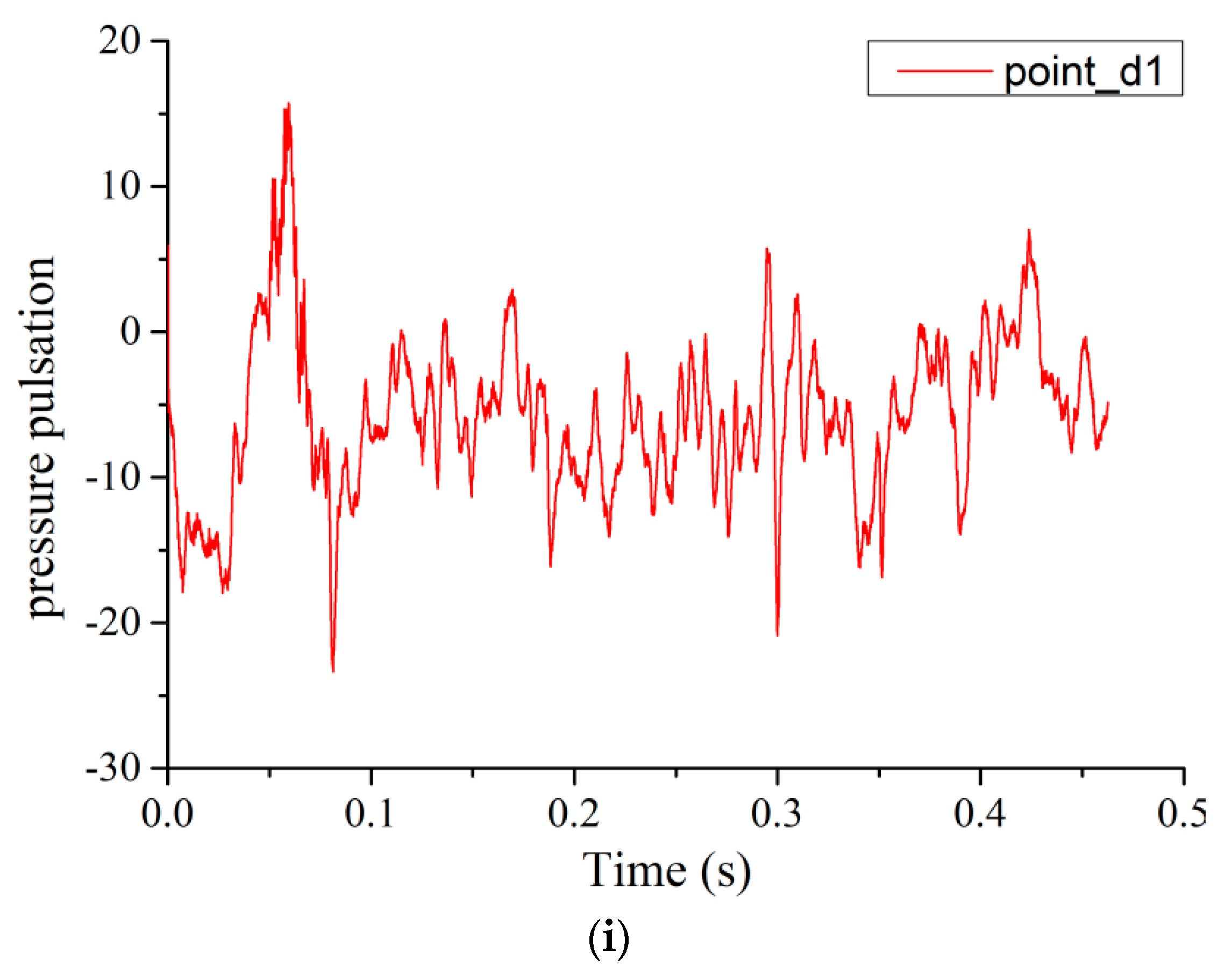
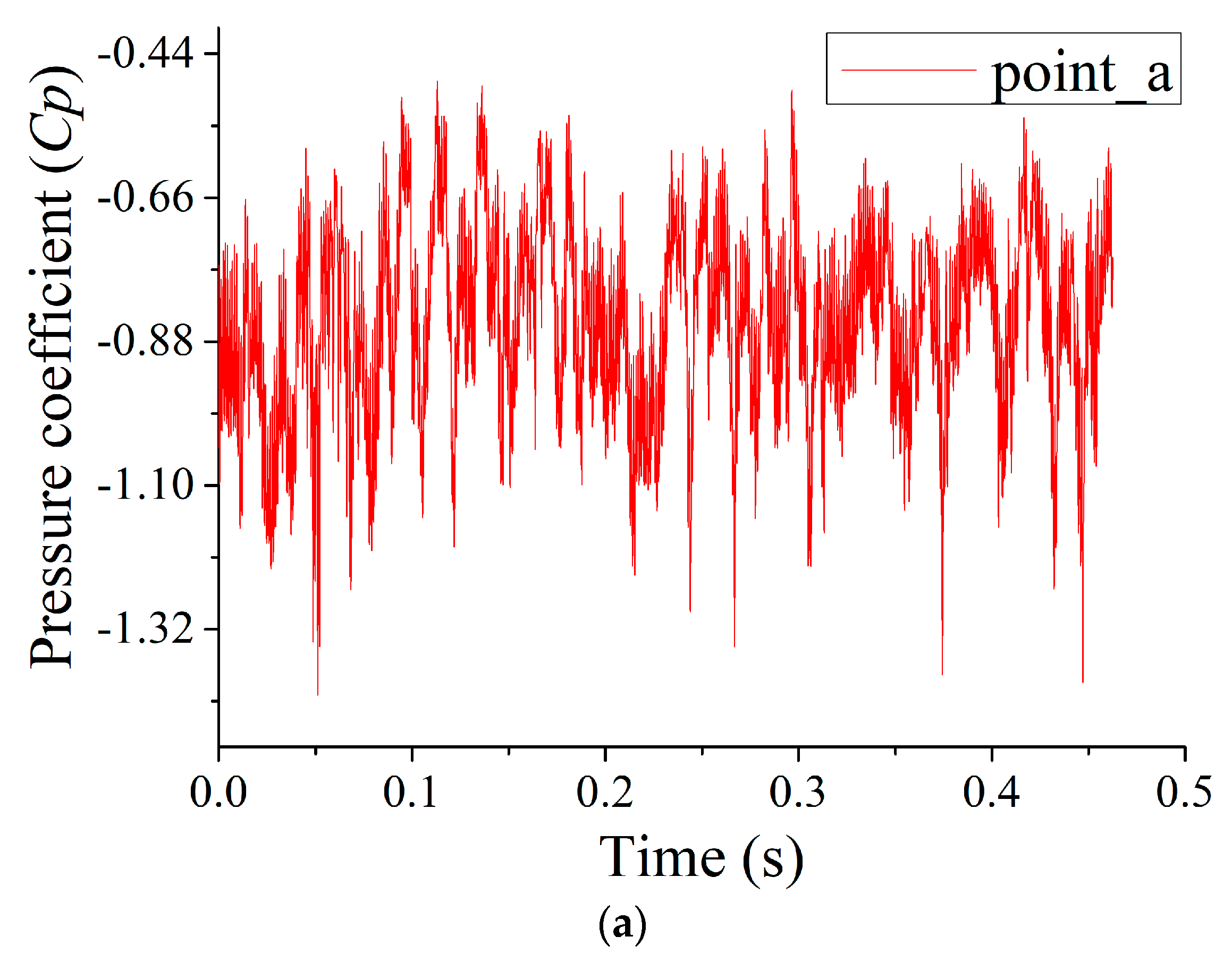
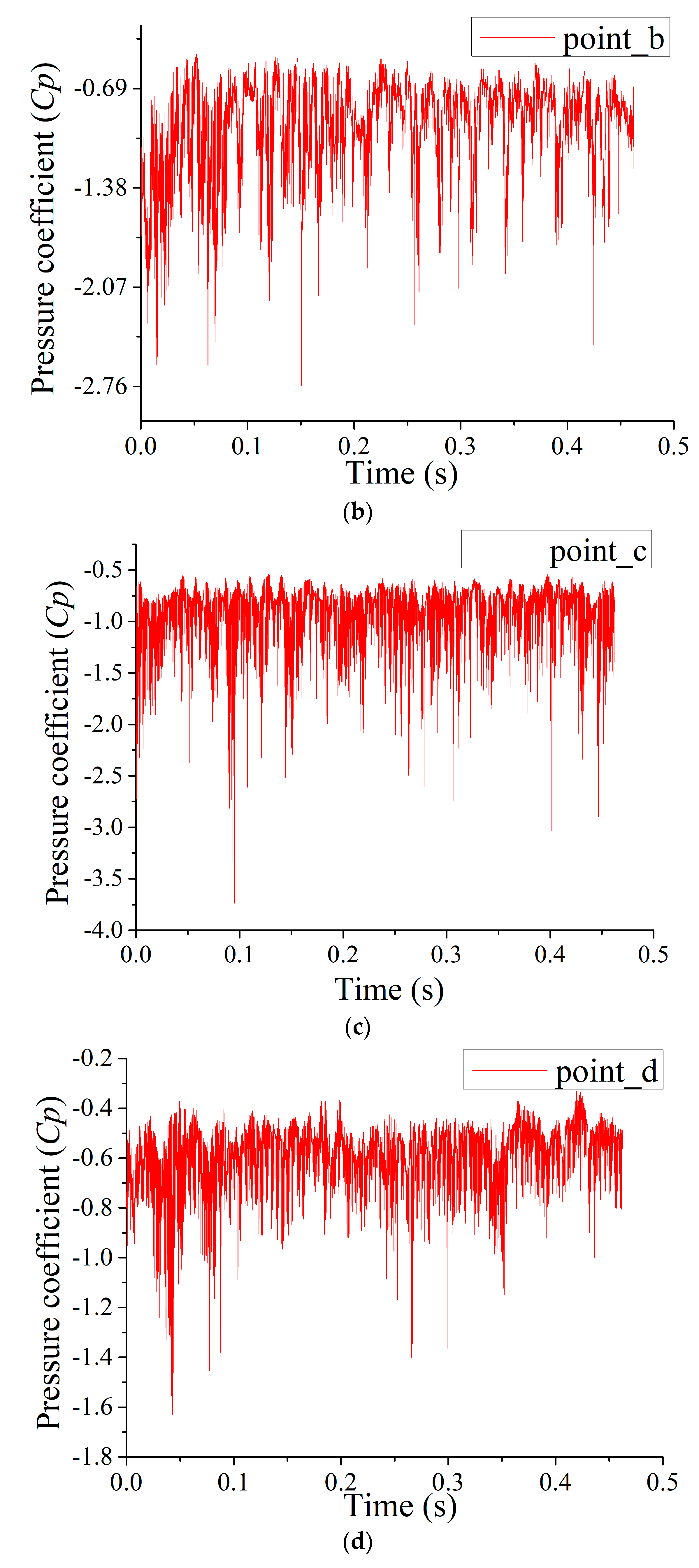
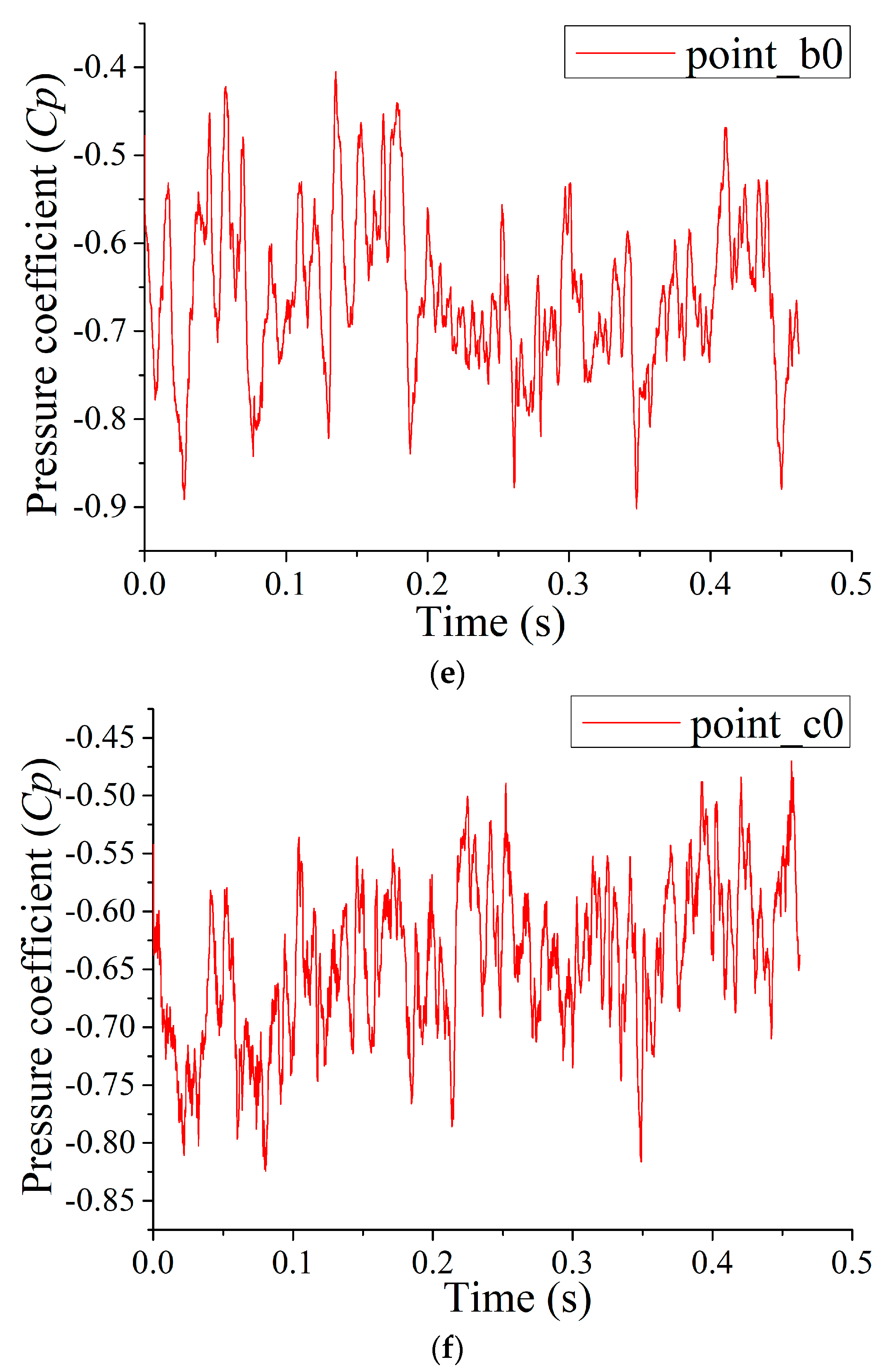
3.4. Pressure Fluctuation of Internal Flow in Centrifugal Fan

In this subsection, the pressure fluctuation and frequency spectrum at key points are mainly introduced in order to further analyze the internal flow of the centrifugal fan with time at a non-dimensional flow rate of Q/Qn = 0.031.

Figure 22 shows the location of monitoring points on the Z = 0 m plane in the process of unsteady calculation. According to Figure 22, one can obviously see that nine material points are monitored. According to the coordinate system in the drawing, four monitoring points are set at the outlet of the impeller, marked as a, b, c, and d, respectively. Three monitoring points (b1, c1, and d1) are located on the wall of the volute. b0 is the middle of b and b₁, and c₀ is the central position between c and c1. The static pressure monitoring of these nine points is carried out separately; in addition, the velocity of points a, b, c, d, b₀, and c₀ is monitored. The static pressure and velocity data are extracted once at each time-step size.

Figure 23 shows a schematic diagram of the pressure fluctuation at each monitoring point. As we can see from Figure 23, the pressure fluctuation at each monitoring point fluctuates in a certain range. The monitoring points (a, b, c, and d) at the impeller outlet all include the pressure fluctuation caused by the rotating of the blade. Due to the close distance from the volute tongue, the airflow near point A is intricate, so the pressure distribution at point A is unstable, and the regularity is weak. The monitoring points (b₀, c₀, b₁, c₁, and d₁) in the volute channel and on the wall of the volute are far away from the impeller, and the pressure fluctuation at each point is mainly caused by boundary layer separation on the suction surface of the blade, the shedding vortex at the end of the blade and the pulsation of the boundary layer on the volute wall; therefore, no obvious regularity is represented. Figure 22 illustrates that the acceleration of the blade passage makes the gas fluctuate greatly when the airflow flows out of the blade passage. The gas velocity near the volute wall decreases due to the diffusive action of the volute, which leads to the separation of the boundary layer. The velocity of gas is larger when the gas flows out of the blade passage. Since the existence of the volute tongue clearance results in the velocity of gas decreasing rapidly, so the fluctuation of gas near the volute tongue is also larger.

Figure 24 shows the variation of static pressure coefficients at different monitoring points over time variation. Generally, the distribution of static pressure coefficients can be analyzed from the wall pressure gradient. When dCp/dt is greater than 0, the boundary layer flow decelerates until separation occurs. On the contrary, when dCp/dt is less than 0, the boundary layer flow is accelerated, which effectively suppresses the separation. From Figure 24, we can see that the gradient of the static pressure coefficient at the monitoring point is less than 0. Therefore, the flow near the monitoring points is accelerated, and no flow separation occurs inside the volute.

Figure 25 presents the static pressure fluctuation spectrum of each monitoring point. The abscissa is the frequency value, and the ordinate is the pressure fluctuation energy amplitude corresponding to each frequency value. As shown in Figure 25, it is observed that the static pressure fluctuations at each monitoring point show distinct discrete spectrum characteristics on the spectrum. Figure 25a, at the impeller outlet position (a, b, c, and d), the obvious peak amplitudes appear at the low-frequency band (2.16 Hz to 160 Hz) and at 866 Hz, and the amplitudes at 15 Hz and 866 Hz are larger than the others. It is mainly indicated that the shedding vortices occur at the blade tip and the rotating action of the impeller is obvious. Since point c is close to the volute tongue, the amplitude of point c at 866 Hz is obviously higher than that of the other three points due to the periodic impact of flow on the volute tongue. In Figure 25b, we can see that the frequency spectrum of monitoring points b₁, c₁, and d₁ in the volute wall position fluctuates within 2.16 Hz to 160 Hz, but it is not obvious at 866 Hz. Due to the diffusive effect of the volute, the velocity of the airflow near the volute wall is small, and a vortex shedding exists on the volute wall, which leads to the fluctuation of the boundary layer. However, the peak value is not obvious at the basic frequency, but there is a larger peak density at the low-frequency band. In Figure 25c, it is seen that the frequency spectrum of the b₀ and c₀ monitoring points in the volute passage fluctuates from 2.16 Hz to 160 Hz, and the amplitude of monitoring point c₀ occurs at 866 Hz, while the amplitude of b₀ is not obvious. It is shown that the flow separation of the blade and the shedding vortices at the end of the blade also produce pressure fluctuation in the volute passage. In Figure 25d, it is obtained that only monitoring point b has a significant amplitude at 866 Hz. In Figure 25e, it is also noted that the amplitude of point c is larger than that of point c₀, but the amplitude of point c1 is not obvious. It is clearly stated that the closer the impeller outlet, the fluctuation frequency is well consistent with the passage frequency of the blade due to the rotating effect of the impeller.

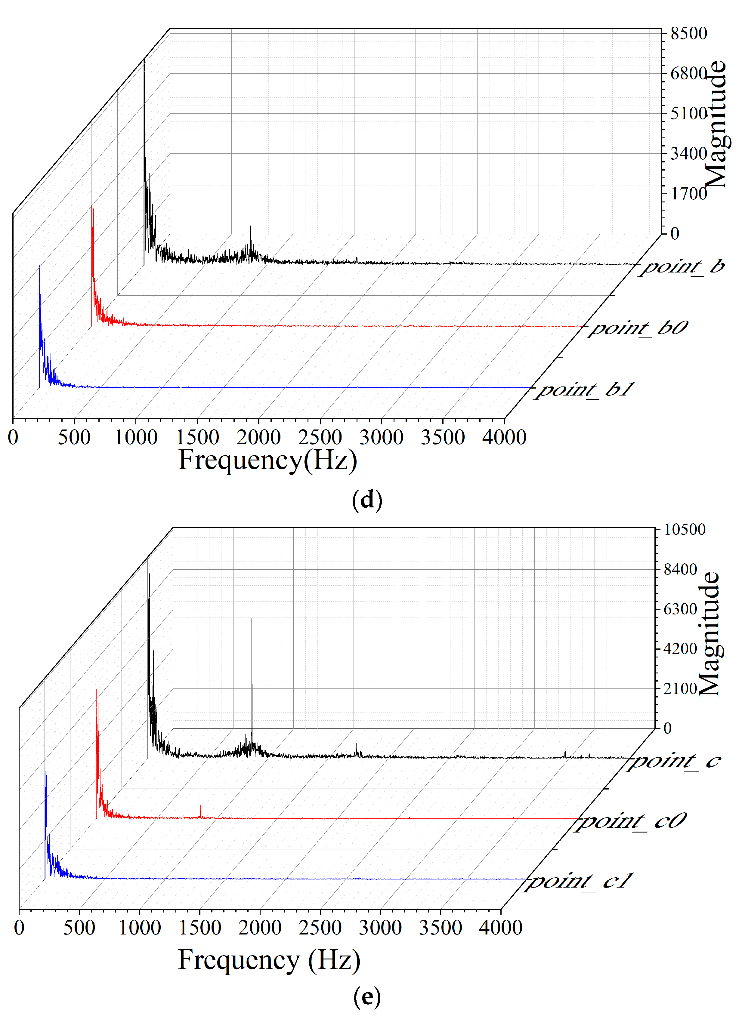
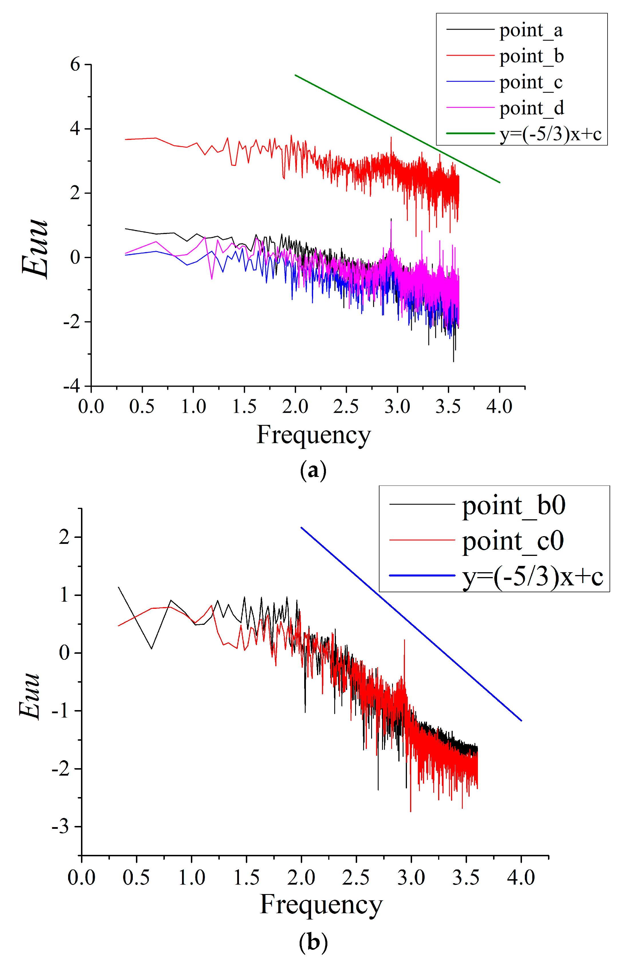
3.5. Kinetic Energy Spectrum of Internal Flow

In this subsection, the internal flow kinetic energy spectrum will be introduced in some critical points of the centrifugal fan. Kolmogorov proposed a statistical theory of locally isotropic turbulence. This theory engenders a famous energy spectrum −5/3 rule of shear turbulence [28].

The drawing of a turbulent flow energy spectrum is divided into three steps. The first step is to obtain the velocity fluctuation (u) at the monitoring point and get the square (u²). The second step is to make a Fourier transform of the square(u²). Finally, the logarithm of the transverse and longitudinal coordinates is used to obtain the kinetic energy spectrum.

Figure 26 exhibits the kinetic energy spectrum of monitoring points on the Z = 0 m plane (logarithmic coordinates). Figure 26a shows the kinetic energy spectrum of the monitoring points (a, b, c, and d) of the outer diameter of the impeller. As illustrated in Figure 26a, we can see that the energy of each frequency at point b is obviously higher than that at the other three points, because point b is close to the volute outlet, and the tangential direction is consistent with the main flow direction. Four monitoring points have large energy peaks at the wave number of 3. It is obtained that a turbulent flow in a centrifugal fan gradually develops at a range of frequency from 10^0.2 to 10^1.7. A full turbulent flow in a centrifugal fan occurs at a range of frequency from 10^1.7 to 10³, which is well consistent with the rake ratio(–5/3) rule of shear turbulence. A turbulent dissipation flow in a centrifugal fan occurs at a range of frequency from 10³ to 10^3.7. Figure 25b shows the kinetic energy spectrum of the monitoring points (b₀,c₀) inside the volute. The wave number range from 10^0.2 to 10^1.7 is a turbulent region; between the 10^1.7 and 10³ wave numbers, it is a complete turbulent region that presents obvious turbulent characteristics. A large energy peak appears at the wave number of 10³. Compared with the monitoring points at the outlet of the impeller and the internal monitoring points of the volute, the internal monitoring points of the volute are more satisfied with the rake ratio (–5/3) rule of shear turbulence.

4. Conclusions

The unsteady internal flow characteristic was researched under a low flow rate by means of large eddy simulation based on computational fluid dynamics. Through the analysis of its internal flow, it is found that the flow instability does exist under the condition of a small flow rate.

First of all, it is can be clearly observed that the internal Q value distribution of a centrifugal fan at different times on the Z = 0.015 m surface is significantly higher near the volute exit and volute tongue. This indicates that the flow instability appears at the volute exit and volute tongue.

In addition, the Q value is higher near the suction surface of the blade and at the end of the blade. This also shows that when airflow flows through the blade passage, flow separation appears around the suction surface, and an evident vortex exists at the blade trailing edge. As the impeller rotates, the airflow from the blade passage falls off at the blade tail, and it gradually becomes apparent. The boundary layer separation near the suction surface and the shedding vortices at the end of the blade will cause a pulsating reaction in the volute port.

What’s more, the pressure fluctuation at each monitoring point shows periodic variation, and its frequency spectrum exhibits obvious discrete characteristics. The frequency spectrum of each monitoring point indicates that the fluctuation frequency is consistent with the fundamental frequency of impeller rotation near the impeller position. The farther away from the impeller position, the higher the density peak appears at the lower frequency band instead of at the fundamental frequency band due to the influence of the blade-shedding vortices and the boundary layer fluctuation on the volute wall.

Finally, for the impeller outlet monitoring points (a, b, c, and d) and the volute channel internal monitoring points (b₀, c₀) similarly, a full turbulent flow in a centrifugal fan occurs at a range of frequencies from 10^1.7 to 10³, which is well consistent with the −5/3 rule of shear turbulence.

References

1. Lee, S.; Kim, H.J.; Runchal, A. Large eddy simulation of unsteady flows in turbomachinery. Proc. Inst. Mech. Eng. Part A J. Power Energy 2004, 218, 463–475. [Google Scholar] [CrossRef]
2. Conway, S.; Caraeni, D.; Fuchs, L. Large eddy simulation of the flow through the blades of a swirl generator. Int. J. Heat Fluid Flow 2001, 21, 664–673. [Google Scholar] [CrossRef]
3. Tajadura, R.-B.; Suarez, V.-S.; Cruz, J.-P.-H.; Morros, C.-S. Numerical calculation of pressure fluctuations in the volute of a centrifugal fan. J. Fluids Eng. 2006, 128, 359–369. [Google Scholar] [CrossRef]
4. Younsi, M.; Bakir, F.; Kouidri, S.; Rey, R. Numerical and experimental study of unsteady flow in centrifugal fan. In Proceedings of the 7th European Turbomachinery Conference, Athens, Greece, 5–9 March 2007; pp. 175–189. [Google Scholar]
5. Younsi, M.; Bakir, F.; Kouidri, S.; Rey, R. 2D and 3D unsteady flow in squirrel-cage centrifugal fan and aeroacoustic behaviour. In Proceedings of the FEDSM2006-98457, ASME Joint US–European Fluids Engineering Summer Meeting, Miami, FL, USA, 17–20 July 2006; pp. 805–813. [Google Scholar]
6. Kato, C.; Kaiho, M.; Manabe, A. An overset finite-element large eddy simulation method with application to turbomachinery and aeroacoustics. J. Appl. Mech. 2003, 70, 32–43. [Google Scholar] [CrossRef]
7. Moon, Y.J.; Cho, Y.; Nam, H.S. Computation of unsteady viscous flow and aeroacoustic noise of cross flow fans. Comput. Fluids 2002, 32, 995–1015. [Google Scholar] [CrossRef]
8. Velarde, S.S.; Ballesteros, T.R.; Santolaria, M.C. Unsteady Flow Pattern Characteristics Downstream of a Forward-Curved Blades Centrifugal Fan. J. Fluids Eng. 2001, 123, 265–272. [Google Scholar] [CrossRef]
9. Yang, J.; Meng, L.; Zhou, L.J.; Luo, Y.Y.; Wang, Z.W. Unsteady internal flow field simulations in a double suction centrifugal fan. Eng. Comput. 2013, 30, 345–356. [Google Scholar] [CrossRef]
10. Wei, Y.K.; Yang, H.; Lin, Z.; Wang, Z.D.; Qian, Y.H. A novel two-dimensional coupled lattice Boltzmann model for thermal incompressible flows. Appl. Math. Comput. 2018, 339, 556–567. [Google Scholar] [CrossRef]
11. Deardorff, J.W. A Numerical Study of Three-Dimensional Turbulent Channel Flow at Large Reynolds Number. J. Fluid Mech. 1970, 41, 453–480. [Google Scholar] [CrossRef]
12. Germano, M.; Piomelli, U.; Moin, P. A Dynamic Subgrid Scale Eddy Viscosity Model. Phys. Fluids A 1991, 3, 1760–1765. [Google Scholar] [CrossRef]
13. Liang, H.; Li, Y.; Chen, J.X.; Xu, J.R. Axisymmetric lattice Boltzmann model for multiphase flows with large density ratio. Int. J. Heat Mass Transf. 2019, 130, 1189–1205. [Google Scholar] [CrossRef]
14. Zhang, W.; Chen, X.P.; Yang, H.; Liang, H.; Wei, Y.K. Forced convection for flow across two tandem cylinders with rounded corners in a channel. Int. J. Heat Mass Transf. 2019, 130, 1053–1069. [Google Scholar] [CrossRef]
15. Lilly, D.K. A Proposed Modification of The Germano sub-grid scaleclosure method. Phys. Fluids A 1992, 4, 633–635. [Google Scholar] [CrossRef]
16. Meneveau, C.; Lund, T.S.; Cabot, W.H. A Lagrangian Dynamic Subgrid Scale Model of Turbulence. J. Fluid Mech. 1996, 319, 353–385. [Google Scholar] [CrossRef]
17. Piomelli, U. High Reynolds Number Calculations Using The Dynamic Subgrid Scale Stress Model. Phys. Fluids 1993, 5, 1484–1490. [Google Scholar] [CrossRef]
18. Bardina, J.; Ferziger, J.H.; Reynolds, W.C. Improved subgrid scale models for large eddy simulation. Am. Inst. Aeronaut. Astronaut. 1980, 80, 13–57. [Google Scholar]
19. Zhou, H.; Cai, G.B. Research of wall roughness effects based on Q criterion. Microfluid. Nanofluid. 2017, 21, 1–14. [Google Scholar] [CrossRef]
20. Li, X.J.; Gao, P.L.; Zhu, Z.C.; Li, Y. Effect of the blade loading distribution on hydrodynamic performance of a centrifugal pump with cylindrical blades. J. Mech. Sci. Technol. 2018, 32, 1161–1170. [Google Scholar] [CrossRef]
21. Zhang, S.F.; Li, X.J.; Hu, B.; Liu, Y.; Zhu, Z.C. Numerical investigation of attached cavitating flow in thermosensitive fluid with special emphasis on thermal effect and shedding dynamics. Int. J. Hydrogen Energy 2019, 44, 3170–3184. [Google Scholar] [CrossRef]
22. Kolář, V.; Šístek, J. Corotational and Compressibility Aspects Leading to a Modification of the Vortex-Identification Q-Criterion. AIAA J. 2015, 53, 2406–2410. [Google Scholar] [CrossRef]
23. Sipp, D.; Jacquin, L. A Criterion of Centrifugal Instabilities in Rotating Systems. Lect. Notes Phys.-N. Y. Berl. 2000, 55, 293–302. [Google Scholar]
24. Billant, P.; Gallaire, F. Generalized Rayleigh criterion for non-axisymmetric centrifugal instabilities. J. Fluid Mech. 2005, 542, 365–377. [Google Scholar] [CrossRef]
25. Lun, Y.X.; Lin, L.M.; He, H.J.; Zhu, Z.C.; Wei, Y.K. Effects of Vortex Structure on Performance Characteristics of a Multiblade Fan with Inclined tongue. Proc. Inst. Mech. Eng. Part A J. Power Energy 2019, 233, 1007–1021. [Google Scholar] [CrossRef]
26. Wang, C.; Hu, B.; Zhu, Y.; Wang, X.; Luo, C.; Cheng, L. Numerical study on the gas-water two-phase flow in the self-priming process of self-priming centrifugal pump. Processes 2019, 7, 330. [Google Scholar] [CrossRef]
27. Wang, C.; He, X.; Zhang, D. Numerical and experimental study of the self-priming process of a multistage self-priming centrifugal pump. Int. J. Energy Res. 2019, 43, 1–19. [Google Scholar] [CrossRef]
28. Kolmogorov, A.N. The Local Structure of Turbulence in Incompressible Viscous Fluid for Very Large Reynolds Numbers. C.R. Acad. Sci. U.R.S.S. 1941, 30, 301–312. [Google Scholar] [CrossRef]
29. Li, X.J.; Jiang, Z.W.; Zhu, Z.C.; Si, Q.R.; Li, Y. Entropy generation analysis for the cavitating head-drop characteristic of a centrifugal pump. Proc. Inst. Mech. Eng. Part C J. Mech. Eng. Sci. 2018, 232, 4637–4646. [Google Scholar] [CrossRef]
30. Liu, Q.; Ye, J.H.; Zhang, G.; Lin, Z.; Xu, H.; Jin, H.; Zhu, Z. Study on the metrological performance of a swirlmeter affected by flow regulation with a sleeve valve. Flow Meas. Instrum. 2019, 67, 83–94. [Google Scholar] [CrossRef]
31. Liu, Q.; Ye, J.H.; Zhang, G.; Lin, Z.; Xu, H.; Zhu, Z. Metrological performance investigation of swirl flowmeter affected by vortex inflow. J. Mech. Sci. Technol. 2019, 33, 1–10. [Google Scholar] [CrossRef]
32. Xu, H.; Cantwell, C.D.; Monteserin, C.; Eskilsson, C.; Engsig-Karupet, A.P.; Sherwin, S.J. Spectral/hp element methods: Recent developments, applications, and perspectives. J. Hydrodyn. 2018, 30, 1–22. [Google Scholar] [CrossRef] [Green Version]
33. Xu, H.; Mughal, S.M.; Gowree, E.; Atkin, C.J.; Sherwin, S.J. Destabilisation and modification of Tollmien–Schlichting disturbances by a three-dimensional surface indentation. J. Fluid Mech. 2017, 819, 592–620. [Google Scholar] [CrossRef]
34. Zhang, W.; Li, X.J.; Zhu, Z.C. Quantification of wake unsteadiness for low-Re flow across two staggered cylinders, Proceedings of the Institution of Mechanical Engineers, Part C. J. Mech. Eng. Sci. 2019. [Google Scholar] [CrossRef]
35. Xu, H.; Sherwin, S.J.; Hall, P.; Wu, X. The behaviour of Tollmien–Schlichting waves undergoing small-scale localised distortions. J. Fluid Mech. 2016, 792, 499–525. [Google Scholar] [CrossRef]
36. Xu, H.; Lombard, J.E.; Sherwin, S.J. Influence of localised smooth steps on the instability of a boundary layer. J. Fluid Mech. 2017, 817, 138–170. [Google Scholar] [CrossRef] [Green Version]
37. Zheng, X.; Lin, Z.; Xu, B.Y. Thermal conductivity and sorption performance of nano-silver powder/FAPO-34 composite fin. Appl. Therm. Eng. 2019, 5. [Google Scholar] [CrossRef]
38. Zhu, Y.J.; Yang, Z.W.; Luo, K.H.; Pan, J.F.; Pan, Z.H. Numerical investigation of planar shock wave impinging on spherical gas bubble with different densities. Phys. Fluids 2019, 31, 056101–056109. [Google Scholar]
39. Zhu, Y.J.; Yang, Z.W.; Pan, Z.H.; Zhang, P.G.; Pan, J.F. Numerical investigation of shock-SF6 bubble interaction with different mach numbers. Comput. Fluids 2018, 177, 78–86. [Google Scholar] [CrossRef]
40. Yang, H.; Zhang, W.; Zhu, Z.C. Unsteady mixed convection in a square enclosure with an inner cylinder rotating in a bi-directional and time-periodic mode. Int. J. Heat Mass Transf. 2019, 136, 563–580. [Google Scholar] [CrossRef]
41. Wei, Y.K.; Wang, Z.D.; Dou, H.S.; Qian, Y.H.; Yan, W.W. Simulations of natural convection heat transfer in an enclosure at different Rayleigh number using lattice Boltzmann method. Comput. Fluids 2016, 124, 30–38. [Google Scholar] [CrossRef]
42. Yang, H.; Yu, P.Q.; Xu, J.; Ying, C.L.; Wen, B.C.; Wei, Y.K. Experimental investigations on the performance and noise characteristics of a forward-curved fan with the stepped tongue. Measu. Contr. 2019. [Google Scholar] [CrossRef]
Figure 1. Three-dimensional model of a centrifugal fan.
Processes 07 00691 g001
Figure 2. Laboratory test system.
Processes 07 00691 g002aProcesses 07 00691 g002b
Figure 3. Mesh of compute domain: (a) the overall structural mesh of the centrifugal fan; (b) the mesh of the volute; (c) the mesh of the impeller; (d) the boundary layer of the volute; (e) detail of the mesh near the blade.
Processes 07 00691 g003aProcesses 07 00691 g003b
Figure 4. Static pressure for different numbers of grids.
Processes 07 00691 g004
Figure 5. Q value distribution between Large Eddy Simulation and Reynolds-averaged Navier–Stokes Equations method (RANS) at the same computing time t = 0.0125 s.
Processes 07 00691 g005
Figure 6. Comparison of experimental and numerical results under different volume flow rates.
Processes 07 00691 g006
Figure 7. Different section positions of the centrifugal fan.
Processes 07 00691 g007
Figure 8. Static pressure of cross-sections at different positions (Q/Qn = 0.031).
Processes 07 00691 g008
Figure 9. Streamline of cross-sections at different positions (Q/Qn = 0.031).
Processes 07 00691 g009
Figure 10. Q value distribution of cross-sections at different positions (Q/Qn = 0.031).
Processes 07 00691 g010
Figure 11. Static pressure of cross-sections at different positions (Q/Qn = 1).
Processes 07 00691 g011
Figure 12. Streamline of cross-sections at different positions (Q/Qn = 1).
Processes 07 00691 g012
Figure 13. Q value distribution of cross-sections at different positions (Q/Qn = 1).
Processes 07 00691 g013
Figure 14. Static pressure of cross-sections at different positions (Q/Qn = 1.758).
Processes 07 00691 g014
Figure 15. Streamline of cross-sections at different positions (Q/Qn = 1.758).
Processes 07 00691 g015
Figure 16. Q value distribution of cross-sections at different positions (Q/Qn = 1.758).
Processes 07 00691 g016
Figure 17. Static pressure at different times of Z = 0.015 m section (Q/Qn = 0.031).
Processes 07 00691 g017
Figure 18. Streamline with time evolution at Z = 0.015 m section (Q/Qn = 0.031).
Processes 07 00691 g018
Figure 19. Q value distribution with time evolution at the Z = 0.015 m section (Q/Qn = 0.031).
Processes 07 00691 g019
Figure 20. Q value distribution at different times of blade passage on the Z = 0.015 m section (Q/Qn = 0.031).
Processes 07 00691 g020
Figure 21. Skin friction coefficient of the pressure surface and suction surface of the blade.
Processes 07 00691 g021aProcesses 07 00691 g021bProcesses 07 00691 g021c
Figure 22. Location of monitoring points on the Z = 0 m plane.
Processes 07 00691 g022
Figure 23. Static pressure fluctuation at different monitoring points. (a) at point a, (b) at point b, (c) at point c, (d) at point d, (e) at point b0, (f) at point c0, (g) at point b1, (h) at point c1, (i) at point d1.
Processes 07 00691 g023aProcesses 07 00691 g023bProcesses 07 00691 g023cProcesses 07 00691 g023d
Figure 24. Pressure coefficient at monitoring points under a flow rate of Q/Qn = 0.031. (a) at point a, (b) at point b, (c) at point c, (d) at point d, (e) at point b0, (f) at point c0.
Processes 07 00691 g024aProcesses 07 00691 g024bProcesses 07 00691 g024c
Figure 25. Spectrum characteristics of monitoring points on the Z = 0 m plane. (a) at point a, b, c, and d, (b) at point b1, c1, and d1, (c) at point c0, and b0, (d) at point b, b0, and b1, (e) at point c, c0, and c1.
Processes 07 00691 g025aProcesses 07 00691 g025b
Figure 26. Kinetic energy spectrum of monitoring points on the Z = 0 m plane. (a) at point a, b, c, and d, (b) at point b0 and c0.
Processes 07 00691 g026