CFD-DEM Modeling and Simulation Coupled to a Global Thermodynamic Analysis Methodology for Evaluating Energy Performance: Biofertilizer Industry

Abstract

This work develops a methodology based on real chemical plant data collected from a Nitrogen-Phosphorus-Potassium fertilizer (NPK) cooling rotary drum. By blending thermodynamic variables given by global energy and mass balances with computational fluid dynamics-discrete element method (CFD-DEM) modeling and simulation, the methodology provides an initial approximation to the understanding of heat transfer inside industry rotary coolers. The NPK cooling process was modeled in CFD software Simcenter STAR − CCM + 13.06.011 using a Eulerian–Lagrangian scheme through a coupled CFD-DEM method using one-way coupling. The average temperature of the NPK particles was obtained as well as the average mass flow of the particles dropping as the drum was rotating. The analysis was performed for two-particle diameters (8 and 20 mm) during 17.5 s. The average heat transfer coefficient between the fluid and the NPK particles during the simulated time was obtained. A thermodynamic analysis was carried out using instantaneous energy and mass balances. Prandtl, Nusselt, and Reynolds numbers were obtained for each simulated time step. Finally, through a non-linear regression using the Marquardt method, a correlation between Prandtl, Nusselt, and Reynolds number was developed that allowed analyzing the rotating drum. Results showed that the proposed methodology could serve as a useful tool during the design and analysis of any given rotary cooler, allowing calculation of the heat transfer coefficient and obtaining the process variables that could expand the machine operational capabilities due to the knowledge of the Nusselt number as a function of the drum working parameters.

1. Introduction

Countercurrent rotary drums are commonly used in the bio-organic fertilizer industry for cooling of granular solids that have high internal moisture retention, low thermal conductivity, and hygroscopicity, such as the case of organic fertilizers. They are often made of a long cylindrical shell that rotates upon bearings along its longitudinal axis, which is inclined to the horizontal to induce product motion from the inlet towards the outlet of the cylinder (Figure 1a) [1]. A blower is placed above the product outlet to provide the cold countercurrent airflow needed for cooling. Besides, to promote air-material contact, most drums have lifters, which are fin-like structures placed along the cylinder length that lift the material from the bed and showers it through the air stream as the drum rotates, creating a cross-flow heat transfer scheme (Figure 1a) [1].

The design of a rotary drum relies on designer expertise and experience with the product and the process and the application of certain theoretical principles and empirical correction factors [2]. Drum flights and shells design have an essential effect on the cooling process [3]. During operation, some particles are sliding and rolling along with the drum, while others are being lifted or falling in spreading cascades through the air stream and re-entering the bed at the bottom, giving rise to complex particle dynamics which affect fluid–solid interactions (Figure 1b) [4]. Nevertheless, a better understanding of the heat transfer phenomena in these processes is still needed for process optimization.

NPK grade 15–15–15 (Fertilizer with 15% Nitrogen, 15% Phosphorus, 15% Potassium) is a water-soluble granular fertilizer of 2.7 mm average particle diameter commonly produced in the Colombian biofertilizer industry. After drying, NPK enters a countercurrent rotary cooler at circa 90 °C and must be below 45 °C at the outlet to decrease the likelihood of compaction and agglomeration during curing and packaging, which negatively affects the quality of the product. Operators often achieve outlet temperatures by adjusting operating conditions such as reducing drum inclination angle, drum rotation, NPK feed rate, and fuel mass flow. Once an industrial rotary drum is manufactured and put into operation, however, further geometrical and operational modifications for process optimization are harder to incorporate, since they generally require long plant downtimes not previously accounted for in maintenance schedules, as well as additional design and manufacturing costs for geometry changes. Thus, these measures ensure a decrease in product throughput and an increase in process costs, which ultimately diminish overall company profits. For these reasons, the industry permanently demands alternate low-cost approaches for process optimization.

Computational techniques have been increasingly employed for understanding complex solid–fluid interactions in multiphase flows. Among them, the discrete element method (DEM) has been widely accepted as an effective method in addressing complex inter particle phenomena in problems involving granular materials, such as granular flows and powder mechanics [5]. In recent years, coupled DEM and computational fluid dynamics (CFD) have been used for modeling the interaction between highly packed low-diameter granulated solids and gas/liquid fluids in fluidized beds, tumbling mills, and particle impaction in water reservoirs, among others [6,7,8,9,10,11]. Nevertheless, real industrial processes such as NPK cooling in a rotary drum involve billions of particles which require vast computational power, which is unfeasible in most research centers [12]. Also, the effects of discontinuous or granulated materials on fluid properties (also known as two-way coupling) requires additional convective terms in the fluid’s conservation of mass, momentum, and energy equations. Hence, simulations become much more computationally intensive [13].

To overcome the above difficulties, a methodology was developed that blends thermodynamic variables given by global energy and mass balances with CFD-DEM modeling and simulation that permits an initial approximation to the understanding of heat transfer inside industrial rotary coolers. Initially, the process is modeled as the cooling process of NPK 15–15–15 inside a 50 $\frac{T}{h}$ countercurrent rotary cooler located in a Colombian biofertilizer industry. The drum geometry and lifting flights were based on the industrial-scale design. The rotating drum was analyzed with a Eulerian–Lagrangian scheme using a CFD-DEM one-way coupled physics model corresponding to the airflow and the NPK granulated solid, respectively. Two particle sizes were analyzed: 20 mm and 8 mm diameter NPK spherical particles inside the rotating cooler in a 1 m and 0.1 m drum section length, respectively. The novelties of this work are presented below:

• A CFD-DEM computational model for NPK in the rotary cooler was developed to study the influence of NPK particle diameter on its average temperature along the drum section length; 17.5 s of simulated cooling time was required to validate the results.
• The process average heat transfer coefficient throughout the simulated time was obtained.
• A thermodynamic model of the drum operation was developed using a heat exchanger model, which was fed by the previously found average heat transfer coefficient of the process.
• Through a non-linear regression method, a correlation of dimensionless numbers was obtained which determines, in a given interval, the process operation characteristics.

CFD-DEM models have been used to study many different complex problems involving particle–fluid flow interaction [14,15] and have been found useful to model fluidized beds. The first study using this approach [16] simulated plug flow through horizontal pipes. Since then, many different problems have been solved with this method [17,18,19].

This paper offers a novel approach that mixes thermodynamic analysis (boundary conditions for the cooler), knowledge about the rotary system (geometry, rotational speed), as well as transport phenomena conditions (air velocity, particle size), to develop a methodology able to solve complex problems in the chemical industry. We expect this work to serve as a quick supporting tool for the design or modification of countercurrent rotary coolers in the biofertilizer industry, particularly in cases where new granulated materials are to be employed, or additional product requirements are placed which require changes in the process current operational conditions.

2. Materials and Methods

The NPK cooling process was simulated in CFD software Simcenter STAR − CCM + V.13.06.011 using a Eulerian–Lagrangian scheme through a coupled CFD-DEM method. Momentum, heat, and mass transfer, were exchanged in only one direction to reduce computational costs, also known as one-way coupling. In this method, only the continuous Eulerian phase (air) influences the solid particles. Hence, the effects of the granulated solid on the air, such as displacement, interphase momentum, mass, and heat transfer, are not initially considered in the methodology. The average temperature of NPK particles, as well as their average mass flow falling from the top of the rotating drum during 17.5 s for two-particle diameters (8 and 20 mm), is obtained. These results were then used to calculate the average heat transfer coefficient between the fluid and the NPK particles during the simulated time. Afterward, a thermodynamic analysis was performed using energy, and mass balances of the simulated section of the rotating cooler to obtain the heat transfer coefficient of the process. Also, the instantaneous Prandtl, Nusselt, and Reynolds numbers of the process for each simulated time step were calculated. Finally, through a non-linear regression using the Marquardt method, a correlation between Prandtl, Nusselt, and Reynolds numbers was obtained for the analyzed rotating cooler.

2.1. Mathematical Models

2.1.1. Particle Dynamics

Linear motion description for the NPK granular flow with spherical solid particles is modeled using the DEM since it extends the Lagrangian formulation to account for inter-particle interactions in the particle equations of motion, which are essential in highly loaded flows. The equation of conservation of linear momentum for a DEM particle of mass $m_p$ is given by Equation (1), where ${\mathit{V}}_p$ denotes the instantaneous particle velocity, ${\mathit{F}}_s$ is the resultant of the forces acting on the surface particle, and ${\mathit{F}}_b$ is the resultant of the body forces. These forces are also decomposed according to Equation (2), where ${\mathit{F}}_d$ is the drag force, ${\mathit{F}}_p$ is the pressure gradient force, ${\mathit{F}}_g$ is the gravity force, ${\mathit{F}}_c$ is the contact force from the DEM, and ${\mathit{F}}_{MRF}$ is the force produced by the rotating reference frame.

$$m_p\frac{d{\mathit{V}}_p}{dt}={\mathit{F}}_s+{\mathit{F}}_b$$

(1)

$$\begin{gathered} {\mathit{F}}_s={\mathit{F}}_d+{\mathit{F}}_p \\ {\mathit{F}}_b={\mathit{F}}_g+{\mathit{F}}_c+{\mathit{F}}_{MRF} \end{gathered}$$

(2)

For the solid-fluid interactions, the resultant ${\mathit{F}}_s$ forces represent the momentum transfer from the continuous phase to the particle. The drag force is given by Equation (3), where $\rho$ is the density of the continuous phase, $A_p$ is the projected area of the particle, ${\mathit{V}}_s$ is the particle slip velocity, and $C_d$ is the drag coefficient of the particle given by the Schiller–Naumann correlation, which is suitable for spherical solid particles. The pressure gradient force ${\mathit{F}}_p$ is defined according to Equation (4), where $V_p$ is the volume of the particle and $\nabla p_{static}$ is the gradient of the static pressure in the continuous phase.

$${\mathit{F}}_d=\frac{1}{2}{C}_d\rho A_p\left|{\mathit{V}}_s\right|{\mathit{V}}_s$$

(3)

$${\mathit{F}}_p=-V_p\nabla p_{static}$$

(4)

For the particle body forces, the gravity force is given by Equation (5), where $\mathit{g}$ is the gravitational acceleration vector. The contact force ${\mathit{F}}_c$ represents inter-particle and particle-boundary interaction and is presented in Equation (6), where ${\mathit{F}}_{cm}$ is the contact force model. A modification of the linear spring contact model developed by Cundall and Strack was used [20].

$${\mathit{F}}_g=m_p\mathit{g}$$

(5)

$${\mathit{F}}_c={\displaystyle \sum }_{contact}{\mathit{F}}_{cm}$$

(6)

The normal and tangential forces are defined by Equation (7), where $K_n$ is the normal spring constant, $K_t$ is the tangential spring constant, $N_n$ is the normal damping, ${\nu }_n$ is the normal velocity component of the relative sphere surface velocity at the contact point, $C_{fs}$ is the static friction coefficient, and $d_n$ and $d_t$ are overlaps in the normal and tangential directions at contact points.

$$\begin{gathered} {\mathit{F}}_n=-K_n{d}_n-N_n{\nu }_n \\ {\mathit{F}}_t=-K_t{d}_t-N_t{v}_t if ⎡K_t{d}_t⎤<⎡K_n{d}_n⎤C_{fs}, otherwise {\mathit{F}}_t=-\frac{\left|K_n{d}_n\right|C_{fs}{d}_t}{\left|d_t\right|} \end{gathered}$$

(7)

The normal and tangential spring stiffness is given by Equation (8). $E_{eq}$, $G_{eq}$, and $R_{eq}$ are the equivalent Young’s modulus, shear modulus, and radius of the interacting particles, and they are calculated according to Equation (9), where $E_A$ and $E_B$ are Young’s modulus of the particles, $v_A$, and $v_B$ their Poisson’s ratios, and $R_A$ and $R_B$ their radii.

$$\begin{gathered} K_n=\frac{4}{3}{E}_{eq}\sqrt{d_n}{R}_{eq} \\ {K}_t=8G_{eq}\sqrt{d_t}{R}_{eq} \end{gathered}$$

(8)

$$\begin{gathered} E_{eq}=\frac{1}{\frac{1-v_A^2}{E_A}+\frac{1-v_B^2}{E_B}} \\ {G}_{eq}=\frac{1}{\frac{2\left(2-v_A\right)\left(1+v_A\right)}{E_A}+\frac{2\left(2-v_B\right)\left(1+v_B\right)}{E_B}} \\ {R}_{eq}=\frac{1}{\frac{1}{R_A}+\frac{1}{R_B}} \end{gathered}$$

(9)

The normal and tangential damping is given by Equation (10), where $N_{n}damp$ and $N_{t}damp$ are the normal and tangential damping coefficient, and $M_{eq}$ is the equivalent particle mass. The normal and tangential coefficients and equivalent particle mass are given by Equation (11), where $C_{nrest}$ and $C_{trest}$ are the normal and tangential coefficients of restitution defined by the physical properties of the material, and $M_A$ and $M_B$ the mass of each colliding particle.

$$\begin{gathered} N_n=2N_{n}damp\sqrt{K_n}{M}_{eq} \\ {N}_t=2N_{t}damp\sqrt{K_t}{M}_{eq} \end{gathered}$$

(10)

$$\begin{gathered} N_{n}damp=\frac{-ln\left(C_{nrest}\right)}{\sqrt{{\pi }^2+ln{\left(C_{nrest}\right)}^2}} \\ {N}_{t}damp=\frac{-ln\left(C_{trest}\right)}{\sqrt{{\pi }^2+ln{\left(C_{trest}\right)}^2}} \\ {M}_{eq}=\frac{1}{\frac{1}{M_A}+\frac{1}{M_B}} \end{gathered}$$

(11)

The force produced by the moving reference frame is given by Equation (12), where $\mathit{\omega }$ is the angular velocity vector of the rotating reference frame and $r$ is the distance vector to the axis of rotation.

$${\mathit{F}}_{MRF}=m_p\left[\mathit{\omega }\times \left(\mathit{\omega }\times r\right)+2\left(\mathit{\omega }\times {\mathit{V}}_p\right)\right]$$

(12)

Rotational motion for DEM particles is described by orientations and, therefore, their angular momentum must also be conserved, and it is represented by Equation (13), where ${\mathit{I}}_p$ is the particle moment of inertia described by a second-order tensor, ${\mathit{w}}_p$ is the particle angular velocity, ${\mathit{M}}_b$ is the drag torque, that is, the moment that acts on the particle due to rotational drag, and ${\mathit{M}}_c$ is the total moment from contact forces.

$${\mathit{I}}_p\frac{d{\mathit{w}}_p}{dt}={\mathit{M}}_b+{\mathit{M}}_c$$

(13)

The drag torque reduces the difference between a particle and the fluid in which it is immersed, and is defined by Equation (14), where $C_R$ is the rotational drag coefficient. $\mathsf{\Omega }$ is the relative angular velocity of the particle to the fluid and is given by Equation (15), where $v$ is the fluid velocity, and ${\mathit{w}}_p$ is the angular velocity of the particle. The rotational drag coefficient is defined by Equation (16) where $R{e}_R$ is the rotational Reynolds number defined by Equation (17).

$${\mathit{M}}_b=\frac{\rho }{2}{\left(\frac{D}{2}\right)}^5{C}_R\left|\mathsf{\Omega }\right|\mathsf{\Omega }$$

(14)

$$\mathsf{\Omega }=\frac{1}{2}\nabla \mathrm{x}v-{\mathit{w}}_p$$

(15)

$$C_R=\frac{64\pi }{R{e}_R}$$

(16)

$$R{e}_R=\frac{\rho D^2\left|\mathsf{\Omega }\right|}{\mu }$$

(17)

The total moment from contact forces is defined according to Equation (18), where ${\mathit{r}}_c$ is the position vector from the particle center of gravity to the contact point, and ${\mathit{M}}_{cm}$ is the moment that acts on the particle from rolling resistance. Rolling resistance was modeled with the proportional force method with a defined coefficient of rolling resistance ${\mu }_r$.

$${\mathit{M}}_c={\displaystyle \sum }_{contacts}\left({\mathit{r}}_c\times {\mathit{F}}_{cm}+{\mathit{M}}_{cm}\right)$$

(18)

In order to study the heat and mass transfer process inside the cooling rotary drum, the solid-fluid heat transfer needs to be defined properly. The equation of conservation of mass of a material particle is given by Equation (19), where ${\dot{m}}_p$ is the rate of mass transfer to the particle. This term is zero since no evaporation occurs. The particle energy balance is shown in Equation (20), where $Q_{rad}$ represents heat transfer by radiation and $Q_s$ represents heat transfer by other sources, and both of them are negligible in this process.

$$\frac{d{m}_p}{dt}={\dot{m}}_p$$

(19)

$$m_p{c}_p\frac{d{T}_p}{dt}=Q_t+Q_{rad}+Q_s$$

(20)

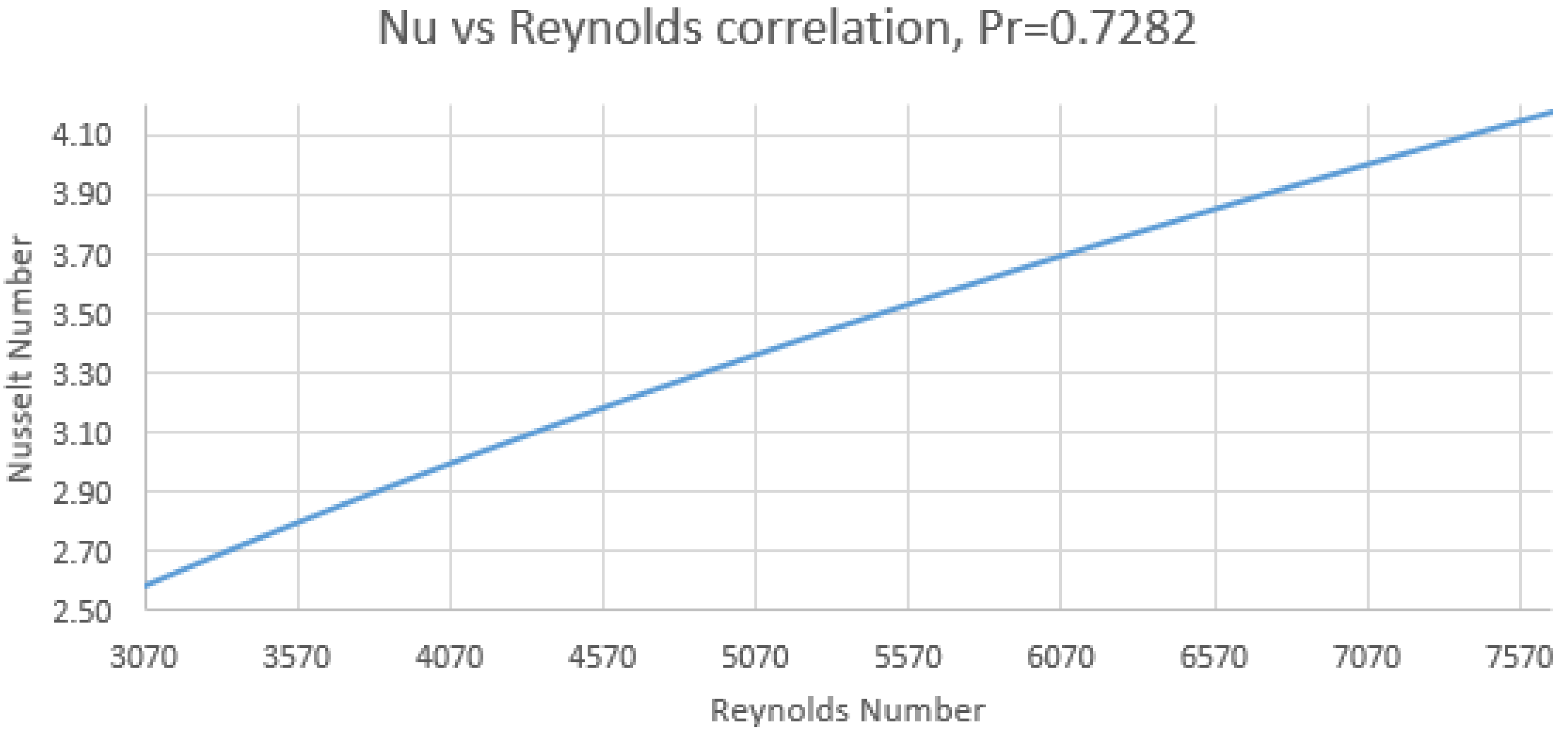
Convective heat transfer $Q_t$ is calculated according to Equation (21), where $h$ is the heat transfer coefficient, and $A_s$ is the particle surface area. The heat transfer coefficient was obtained from the particle Nusselt number presented in Equation (22), where $k$ is the thermal conductivity of the fluid. Nusselt number was obtained using the Ranz–Marshall correlation defined by Equation (23), where $Pr$ is the Prandtl number of the air.

$$Q_t=h{A}_s\left(T-T_p\right)$$

(21)

$$N{u}_p=h\frac{D_p}{k_f}$$

(22)

$$N{u}_p=2\left(1+0.3R{e}_p^{0.5}P{r}^{1/3}\right)$$

(23)

The solid-solid heat transfer process is taken into consideration. When particles make contact with each other or with the wall, heat is transferred through conduction. In this work, the drum wall was considered adiabatic. Thus, conductive heat transfer was only considered between particles. Particle–particle heat transfer is given by Equation (24), where $r_c$ is the contact radius and $k$ is the equivalent thermal conductivity of the two particles and $T_i, T_j$ the temperatures of particle i and j. The equivalent thermal conductivity is calculated according to Equation (25), where $k_i$ and $k_j$ are the thermal conductivities for particles i and j.

$$q_{ij}=4r_c{k}_m\left(T_j-T_i\right)$$

(24)

$$\frac{1}{k}=\frac{1}{k_i}+\frac{1}{k_j}$$

(25)

The impact heat model was employed for calculating the heat production that results from friction and damping in DEM particles. This model has a linear formulation given by Equation (26), where $c_t$ and $c_n$ are the fractions of frictional and damping work that are converted to heat, $f_t$ and $f_n$ are the frictional and damping forces on the particle, and $v_t$ and $v_n$ are the relative tangential and normal impact velocities.

$$q_r=c_t{f}_t{v}_t+c_n{f}_n{v}_n$$

(26)

2.1.2. Fluid Dynamics

Air was modeled as a constant density gas using a Eulerian scheme. The equations of conservation of mass, momentum, and energy were solved with mesh motion, which provides an additional flux in the convective terms. This set of equations is defined by Equation (27), where ${\mathit{\nu }}_g$ is the grid velocity in the reference frame and ${\mathit{\nu }}_r$ is the relative velocity with respect to the reference frame, $\mathit{\sigma }$ is the stress tensor, ${\mathit{f}}_b$ is the resultant body forces (gravity), $E$ is the total energy per unit mass, $\mathit{q}$ is the heat flux and $S_u$ and $S_e$ are mass and energy sources

$$\begin{gathered} \frac{\partial }{\partial t}\underset{V}{{\displaystyle \int }}\rho dV+{{\displaystyle \oint }}_A\rho \left({\mathit{\nu }}_r-{\mathit{\nu }}_g\right)·d\mathit{a}=\underset{V}{{\displaystyle \int }}{S}_{u}dV \\ \frac{\partial }{\partial t}\underset{V}{{\displaystyle \int }}\mathit{\rho }\mathit{\nu }\mathit{d}\mathit{V}+{{\displaystyle \oint }}_A\rho \mathit{\nu }\otimes \left({\mathit{\nu }}_r-{\mathit{\nu }}_g\right)·d\mathit{a}={{\displaystyle \oint }}_A\mathit{\sigma }·d\mathit{a}+\underset{V}{{\displaystyle \int }}{\mathit{f}}_{b}dV-\underset{V}{{\displaystyle \int }}\rho \mathit{\omega }\times \mathit{\nu }dV \\ \frac{\partial }{\partial t}\underset{V}{{\displaystyle \int }}\mathit{\rho }E\mathit{d}\mathit{V}+{{\displaystyle \oint }}_A\rho E\left({\mathit{\nu }}_r-{\mathit{\nu }}_g\right)·d\mathit{a}=-{{\displaystyle \oint }}_A\mathit{q}·d\mathit{a}+{{\displaystyle \oint }}_A\left(\mathit{\nu }·\mathit{\sigma }\right)·d\mathit{a}+\underset{V}{{\displaystyle \int }}{\mathit{f}}_b·\mathit{\nu }dV+\underset{V}{{\displaystyle \int }}{S}_{e}dV \end{gathered}$$

(27)

When the mesh is moving, cells shape and position change with time. Hence, an additional equation was solved to enforce space conservation, described by Equation (28).

$$\frac{d}{dt}\underset{V}{{\displaystyle \int }}d\mathit{V}=\underset{A}{{\displaystyle \int }}{\mathit{\nu }}_g·d\mathit{a}$$

(28)

2.1.3. Turbulence Model

Turbulence was modeled with the realizable k-ɛ model, which exhibits superior performance for flows involving rotation than the k-ɛ turbulence model. This model added two equations which solve the turbulent kinetic energy $k_e$ and turbulent energy dissipation rate $ϵ$ [21], which are given by Equation (29):

$$\begin{gathered} \frac{\partial }{\partial t}\left(\rho k_e\right)+\frac{\partial }{\partial x_j}\left(\rho k_e{u}_j\right)=\frac{\partial }{\partial x_j}\left[\left(\mu +\frac{{\mu }_t}{{\sigma }_k}\right)\frac{\partial k_e}{\partial x_j}\right]+P_k+P_b-\rho ϵ-Y_M+S_k \\ \frac{\partial }{\partial t}\left(\rho ϵ\right)+\frac{\partial }{\partial x_j}\left(\rho ϵu_j\right)=\frac{\partial }{\partial x_j}\left[\left(\mu +\frac{{\mu }_t}{{\sigma }_{ϵ}}\right)\frac{\partial ϵ}{\partial x_j}\right]+\rho C_1{S}_{ϵ}-\rho C_2\frac{{ϵ}^2}{k_e+\sqrt{\nu ϵ}}+C_{1ϵ}\frac{ϵ}{k_e}{C}_{3ϵ}{P}_b+S_{ϵ} \end{gathered}$$

(29)

In these equations, $S$ is the modulus of the mean rate-of-strain tensor, $P_k$ represents the generation of turbulence kinetic energy due to the mean velocity gradients, calculated in the same manner as standard k-ɛ model, and $P_b$ is the generation of turbulence kinetic energy due to buoyancy, calculated in the same way as standard k-ɛ model [21,22]. $C_1$, $\eta$ and $S$ and $\mu$ are given Equation (30), while the turbulent viscosity is defined by Equation (31) and the terms required are defined in Equation (32).

$$\begin{gathered} C_1=max\left[0.43,\frac{\eta }{\eta +5}\right] \\ \eta =max\left[S\frac{k_e}{ϵ}\right] \\ S=\sqrt{2S_{ij}{S}_{ij}} \end{gathered}$$

(30)

$${\mu }_t=\rho C_{\mu }\frac{k_e{}^2}{ϵ}$$

(31)

$$\begin{gathered} C_{\mu }=\frac{1}{A_0+A_s\frac{k_e{U}^{*}}{ϵ}} \\ {U}^{*}=\sqrt{S_{ij}{S}_{ij}+{\tilde{\mathsf{\Omega }}}_{ij}{\tilde{\mathsf{\Omega }}}_{ij}} \\ {\tilde{\mathsf{\Omega }}}_{ij}={\mathsf{\Omega }}_{ij}-2{ϵ}_{ijk}{\omega }_k \\ {\mathsf{\Omega }}_{ij}=\overline{{\mathsf{\Omega }}_{ij}}-{ϵ}_{ijk}{\omega }_k \end{gathered}$$

(32)

The final terms defining the turbulence model are presented in Equation (32), where $\overline{{\mathsf{\Omega }}_{ij}}$ is the mean rate-of-rotation tensor viewed in a rotating reference frame with the angular velocity ${\omega }_k$, and the model constants $A_0$ and $A_s$ are given by Equation (33).

$$\begin{gathered} A_0=4.04 \\ {A}_s=\sqrt{6}cos\left(\varphi \right) \\ \varphi =\frac{1}{3}co{s}^{-1}\left(\sqrt{6}W\right) \\ W=\frac{S_{ij}{S}_{jk}{S}_{ki}}{{\tilde{S}}^3} \\ \tilde{S}=\sqrt{S_{ij}{S}_{ij}} \\ {S}_{ij}=\frac{1}{2}\left(\frac{\delta u_j}{\delta x_i}+\frac{\delta u_i}{\delta x_j}\right) \\ {C}_{1ϵ}=1.44 \\ {C}_2=1.8 \\ {\sigma }_k=1.0 \\ {\sigma }_{ϵ}=1.2 \end{gathered}$$

(33)

2.2. Heat-Transfer Model

The average NPK temperature is used for each time step to obtain the heat-transfer coefficient between air and solid particles. NPK average temperature differential is given by Equation (34), where $dt$ is the simulation timestep, ${\overline{T}}_{t+dt}$ is the average NPK temperature in time $t+dt$ and ${\overline{T}}_t$ is the average NPK temperature in time $t$.

$$d{\overline{Tm}}_{t+dt}={\overline{T}}_{t+dt}-{\overline{T}}_t$$

(34)

Heat transfer between NPK and air is assumed to occur mostly during PK falling from the flights during drum rotation. Hence, NPK thermal energy is defined by Equation (35), where ${\overline{m}}_{mf}$ is the average NPK mass that falls during one time step. It is assumed that this energy is given to the flowing air, increasing its temperature accordingly. Thus, the air temperature differential is defined by Equation (36), where ${\overline{m}}_a$ is the air mass passing during one time step, and $C{p}_a$ is the air-specific heat. The final expression for air temperature after one time step is given by Equation (37), where $T_{ai}$ is the air temperature at the inlet.

$$Q{m}_{t+dt}={\overline{m}}_{mf}C{p}_{m}d{\overline{T}}_{t+dt}$$

(35)

$$dT{a}_{t+dt}=\frac{Q{m}_{t+dt}}{m_{a}C{p}_a}$$

(36)

$$T{a}_{t+dt}=T_{ai}+d{\overline{Ta}}_{t+dt}$$

(37)

In order to obtain the average heat-transfer coefficient $h$, the process was modeled as a counter-current heat exchanger. This method is suitable in cases where flow rates and heat transfer area are constant. Thus, a generic heat exchanger was employed with two ends: A, at which the hot material enters, and hot air leaves the system, and B, where cold material leaves and cold air enters the system. The logarithmic mean temperature difference $LMTD$ is defined as the difference between the hot and cold feeds at each end of the countercurrent heat exchanger and is given by Equation (38).

$$LMTD=\frac{\left({\overline{T}}_t-T{a}_{t+dt}\right)-\left({\overline{T}}_{t+dt}-T_{ai}\right)}{ln\left(\frac{{\overline{T}}_t-T{a}_{t+dt}}{{\overline{T}}_{t+dt}-T_{ai}}\right)}$$

(38)

The LMTD was used to determine the heat transfer coefficient $h$ for each timestep in the heat exchanger model, and it is calculated according to Equation (39), where $\frac{dQm}{dt}$ is the heat exchanged between NPK and the air during the defined timestep in the heat exchanger model, and $A_{fp}$ is the area of heat exchange corresponding to the total area of the particles falling during one timestep. This term, the rate of heat transfer $\frac{dQm}{dt}$ during the time step $dt$ is given by Equation (40).

$$h=\frac{\frac{dQm}{dt}}{A_{fp}LTMD}$$

(39)

$$\frac{dQm}{dt}=\frac{Q{m}_{t+dt}}{dt}$$

(40)

The area of heat exchange $A_{fp}$ is given by Equation (41).

$$A_{fp}=\frac{4\pi {\left(\frac{D_p}{2}\right)}^2}{m_p}{\overline{m}}_{mf}$$

(41)

The average heat transfer coefficient for each simulation was found by averaging the heat transfer coefficients of each timestep during the entire simulated time.

2.3. Thermodynamic Model

A global energy balance was used to obtain a generalized thermodynamic model of the cooler. First, the heat was assumed to transfer from the NPK material to the air without loses. Hence, the energy balance is presented by Equation (42), where ${\dot{m}}_a$ and ${\dot{m}}_m$ are the mass flows of air and material entering the rotating cooler, respectively, $T_{ai}$ and $T_{ao}$ the air temperatures at the inlet and outlet, and $T_{mi}$ and $T_{mo}$ the material temperatures at the inlet and outlet. Since NPK inlet and outlet temperatures were known, thermal power is given by Equation (43).

$${\dot{m}}_{a}C{p}_a\left(T_{ao}-T_{ai}\right)={\dot{m}}_{m}C{p}_m\left(T_{mo}-T_{mi}\right)$$

(42)

$$Q_m={\dot{m}}_{m}C{p}_m\left(T_{mo}-T_{mi}\right)$$

(43)

The air outlet temperature was then obtained from Equation (44).

$$T_{ao}=T_{ai}+\frac{Q_m}{{\dot{m}}_{a}C{p}_m}$$

(44)

The heat-transfer coefficient from Section 2.2 was used for both particle diameters in a counter-current heat exchanger model of the entire NPK industrial cooler. The inlet–outlet temperatures were used to in the thermodynamic model to find the exchanged heat in the cooling process, which is calculated from Equation (45).

$$Q_{he}=h{A}_{he}LTM{D}_{he}$$

(45)

$A_{he}$ is the total area for heat exchange, and $LTM{D}_{he}$ is the logarithmic mean temperature difference of the heat exchanger. The total area of heat exchange is defined by Equation (46), where $L$ is the rotating cooler length, and $l$ is the length of the simulated drum model.

$$A_{he}=\frac{4\pi {\left(\frac{D_p}{2}\right)}^2{\overline{m}}_{mf}}{dt m_p}\frac{L}{l}$$

(46)

The logarithmic mean temperature difference is given by Equation (47).

$$LMT{D}_{he}=\frac{\left(T_{mi}-T_{ao}\right)-\left(T_{mo}-T_{ai}\right)}{ln\left(\frac{T_{mi}-T_{ao}}{T_{mo}-T_{ai}}\right)}$$

(47)

Both $Q_m$ and $Q_{he}$ should be equal. Thus, Equation (48) is used as check point.

$$Q_{he}=h{A}_{he}LMT{D}_{he}=Q_m={\dot{m}}_{m}C{p}_m\left(T_{mo}-T_{mi}\right)$$

(48)

Through trial and error, NPK outlet temperature that makes $Q_{he}=Q_m$ was calculated. NPK and air inlet and outlet temperatures obtained from this model were validated with the ones given as boundary conditions in the real industrial rotary cooler.

2.4. Dimensionless Numbers

The Nusselt number and Reynolds number for the NPK material, as well as the Prandtl number for the air for each particle diameter during each time step, were obtained. Particle Nusselt is given by Equation (49).

$$N{u}_m=\frac{h{D}_p}{k}$$

(49)

The Prandtl number of the air was found by linear interpolation of published Prandtl numbers for given air temperatures. The average air temperature was defined according to Equation (50).

$$T_{ma}=\frac{T_{ai}+T{a}_{t+dt}}{2}$$

(50)

NPK Reynolds number was obtained from Equation (51), where $v_{max}$ is the maximum air velocity throughout the drum, and $\nu$ is the air kinematic viscosity at the average air temperature. Air kinematic viscosity was obtained by linear interpolation of published kinematic viscosities for given air temperatures. The maximum air velocity is given by Equation (52), where $V_{ai}$ is the average air inlet velocity and $Vf$ is the void factor, which is defined by Equation (53). $V_d$ is the drum volume, and $V_m$ is the volume occupied by the NPK. The drum volume is calculated according to Equation (54), where D is the drum diameter, and $l$ is the drum length in the simulation.

$$R{e}_m=\frac{v_{max}{D}_p}{\nu \left\{T=T_{ma}\right\}}$$

(51)

$$v_{max}=\frac{V_{ai}}{Vf}$$

(52)

$$Vf=\frac{V_d-V_m}{V_d}$$

(53)

$$V_d=\pi {\left(\frac{D}{2}\right)}^{2}l$$

(54)

The volume occupied by the NPK material is given by Equation (55), where $N$ is the number of NPK particles in the model.

$$V_m=\frac{4}{3}\pi {\left(\frac{D_p}{2}\right)}^{3}N$$

(55)

2.5. Non-Linear Regression for Dimensionless Numbers Correlation

The values of the dimensionless numbers obtained for each particle diameter at each time step were used to find a correlation of the form given by Equation (56), where $a$, $b$, and $c$ are constants that relate the dimensionless numbers. The Marquardt non-linear regression method was used in the software Statgraphics Centurion V16.1 to obtain the values of these constants.

$$Nu=aR{e}^{b}P{r}^c$$

(56)

3. Computational Implementation

3.1. Rotary Cooler Characteristics

A fully operating Colombian industrial NPK rotary cooler was used as a case study for the proposed methodology. The cooler has a diameter of three meters, is 19 meters long, rotates at 5 rpm, and is tilted down 1.5° to the horizontal. Four different flight designs are employed in the industrial drum. The flights are arranged in a defined order along the drum length to complete a total of 13 sections. Atmospheric air is used as cooling fluid and enters the drum using a blower which generates a mass flow of $25\frac{Kg}{s}$ at 30 °C and leaves it at approximately 59 °C. NPK particles enter the drum with a mass flow of $13.88889\frac{Kg}{s}$ at a temperature of 90 °C and leave it at 46.5 °C. Outlet mass flows were measured to be equal to inlet ones. Solid NPK particles have an average diameter of 2.7 mm in the industrial cooler and have a residence time of 30 min. With these values, a total mass of 25,000 kg is found inside the drum at any given time. That amounts to approximately $2.3\times {10}^9$ solid NPK particles. Process parameters are shown in

Table 1. Process parameters. N.r. means not reported, d.a. means do not apply.

	Industry Rotating Cooler	Model One	Model Two
Drum properties
Drum diameter $D\left(m\right)$	3	3	3
Drum length $L\left(m\right), l\left(m\right)$	19	0.1	1
Flight design	four different designs (not shown)	Figure 2
Flight material	Stainless steel	Carbon steel
Wall material	Carbon steel	Carbon steel
Angular velocity $\omega \left(rpm\right)$	5
Fluid properties and flow conditions
Fluid	Air
Inlet pressure $P_i\left(kPa\right)$	101.3
Outlet pressure $P_o\left(kPa\right)$	101.3
Inlet temperature ${\mathrm{T}}_{\mathrm{ai}} \left({}^{°}\mathrm{C}\right)$	30
Outlet temperature ${\mathrm{T}}_{\mathrm{ao}}\left({}^{°}\mathrm{C}\right)$	59	d.a.
Inlet mass flow ${\dot{m}}_{ai}(\frac{kg}{s})$	25	25
Outlet mass flow ${\dot{m}}_{ao}(\frac{kg}{s})$	25	25
Particle properties
Material	NPK granulated solid
Diameter $D_p\left(mm\right)$	2.7	8	20
Young’s Modulus $E\_eq \left(kPa\right)$	n.r.	517
Poisson’s ratio $v$	n.r.	0.45
Specific heat $C_p(\frac{J}{kg k})$	1465.38
Thermal conductivity $k_m (\frac{W}{m K})$	0.18596
Density $\rho \left(\frac{kg}{m^3}\right)$	1050
Residence time $rs\left(min\right)$	30
Total mass $MT\left(kg\right)$	25,000	131.57	1315.78
Number of particles $N$	2.31 × 109	4.67 × 105	2.99 × 105
Inlet mass flow ${\dot{m}}_{mi}(\frac{kg}{s})$	13.88	d.a.
Outlet mass flow ${\dot{m}}_{mo}(\frac{kg}{s})$	13.88	d.a.
Inlet temperature ${\mathrm{T}}_{\mathrm{mi}}\left({}^{°}\mathrm{C}\right)$	90
Outlet temperature ${\mathrm{T}}_{\mathrm{mo}}\left({}^{°}\mathrm{C}\right)$	46.5	d.a.
Phase Interactions
Particle-particle
Static friction coefficient $C_{fsp}$	n.r.	0.4
Normal restitution coefficient $C_{nrestp}$	n.r.	0.1
Tangential restitution coefficient $C_{trestp}$	n.r.	0.1
Frictional work fraction $c_{tp}$	n.r.	0.1
Damping work fraction $c_{np}$	n.r.	0.1
Particle-wall
Static friction coefficient $C_{fsw}$	n.r.	0.2
Normal restitution coefficient $C_{nrestw}$	n.r.	0.3
Tangential restitution coefficient $C_{trestw}$	n.r.	0.3
Frictional work fraction $c_{tw}$	n.r.	0.4
Damping work fraction $c_{nw}$.	n.r.	0.1

.

3.2. Model Description

Considering that computational resources for simulating NPK cooling of such a large number of solid particles were unfeasible to acquire, the drum length was reduced, and particle diameter was increased to obtain a total mass that achieved less than a million particles but still was representative of the cooling process. Hence, two models were developed, one of a one-meter drum section length with 20 mm diameter NPK spherical particles, and one of a 0.1 m section length with 8 mm diameter NPK spherical particles, both tilted down 1.5° to the horizontal.

For 20 mm particles, drum length was reduced considering fluid dynamic conditions, particularly Reynolds number and Pressure coefficient. Reynolds number remained constant and was independent from the length of the drum. Since Reynolds was turbulent, the hydrodynamic entry region was 10 times the drum diameter, resulting in 30 m. With this condition, fully developed turbulent flow could not be achieved. For pressure coefficient, the pressure drop is proportional to the length of the drum presenting a linear behavior. Since a developing region will dominate the phenomenon inside, the length of the drum to be analyzed was dropped to 1 m, which represented 5.2% of the total length, which is well inside the developing region of the process. For 8 mm particles, Fourier number was considered because of the transient situation to be analyzed during the cooling process. For both particle sizes, 20 and 8 mm, Fourier number was held at $4\times {10}^{-3}$. This allowed the calculation of drum length for 8 mm particles’ size.

For these lengths, masses of 1315.789 kg and 131.578 kg of NPK were obtained, formed by 299,164 and 467,443 spheres. Both models used one of the four given types of lifters, which were chosen since they allowed the highest particle dispersion angle (angle between the first and last particle showering from the top of the drum). The geometry of the 0.1 m long rotating cooler and its lifters is shown in Figure 2.

Air inlet and outlet conditions were defined as mass flow inlet and pressure outlet in the software. Values for mass flows, pressures, and temperatures were defined as equal to those currently employed in the industrial cooler. Nevertheless, solid NPK particles did not flow from defined inlet and outlet boundaries. Instead, a random particle injector, a tool inside STAR-CCM+, was used to place particles inside the drum’s fluid region in a randomized fashion with a defined initial temperature equal to the NPK inlet temperature of the industrial cooler. Hence, even though no NPK inlet flow was used, NPK particles were initially set with the industrial cooler NPK inlet temperature.

Wall boundary conditions were chosen for the drum carcass and phase-impermeable conditions for the air inlet and outlet boundaries, so particles could not escape the drum during cooling once they have been randomly injected (Figure 3). Thus, a constant number of particles were randomly positioned inside the drum at the start of the simulation and could not leave the drum. Particle dynamics were obtained by solving the equations found in Section 2.1.1 for the constant number of particles defined in Table 1.

3.3. Simulation

The simulation was run for 17.5 s for each model, which corresponded to 1.45 rotations of NPK particles inside the drum. Longer simulation times did not provide additional information regarding NPK temperature drop dynamics since no considerable differences in average heat transfer coefficients were found. Furthermore, the logarithmic mean temperature difference behavior is well defined at this point, allowing the calculations of the heat to be removed inside the drum during the cooling process. The average air inlet velocity $V_{ai}$ was used for calculating the maximum air velocity $v_{max}$. Average NPK falling mass flow was calculated using the track model in STAR-CCM+, which allowed the tracking of each moving particle throughout time. A plane cutting the drum in half in the y-axis was defined, and the tracked particles which cross it throughout a specified time frame were plotted (Figure 4). The data was then exported to a CSV file, where each row corresponded to each crossing particle and each column to the crossing time and z- position. Particle falling mass flow for each model is given by Equation (57), where $\Delta t$ is the time frame between the first and last particle that passes through the defined plane section. Measurements for ${\overline{\dot{m}}}_{mf}$ were performed in time frames positioned after one second of real simulated time since this time was enough for the initially randomly localized particles to position inside the flights of the rotating drum and produce a quasi-steady falling mass flow.

$${\overline{\dot{m}}}_{mf}=\frac{\#ofparticles}{\Delta t}{m}_p$$

(57)

3.4. Domain Discretization

3.4.1. Mesh Generation

The fluid domain was discretized using three models: surface remesher, trimmer, and prism layer mesher. The first one resulted in a good quality surface mesh by adequately maintaining the drum and flights geometry. Trimmer mesh was employed for generating a predominantly hexahedral mesh with minimal cell skewness and a low number of trimmed cells. This method was sufficient for producing a mesh with appropriate curvature and alignment with the z-direction corresponding to the drum length (Figure 5). Prism layer mesher was used to model the inclusion of a prism layer along the borders of the fluid domain to capture boundary layer flow. Mesh properties are shown in

Table 2. Mesh characteristics for each model.

Model	One			Two
Particle diameter (mm)	8			20
Mesh number	1	2	3	1	2	3
base size (m)	0.0368	0.0300	0.0245	0.0480	0.0400	0.0338
Cells	91,952	146,144	226,565	216,008	336,351	504,635
Faces	264,569	422,248	654,658	632,931	988,663	1,485,106
Vertices	102,434	160,771	244,976	228,135	353,909	526,248
Prism layers	5
Prism layer thickness (m)	0.009
Prism layer stretching	1.5

.

3.4.2. Time and Mesh Independence Analysis

Three different mesh sizes were generated for each model. Each finer mesh had 1.5 times the number of cells of the coarser ones. Convergence criteria were set to ${10}^{-4}$ for momentum, energy, turbulent kinetic energy and turbulent energy rate of dissipation. Initially, a time independence analysis was performed. For it, Mesh number 1 was chosen for each model (

Table 3. Time independence analysis.

Model	One			Two
Particle diameter (mm)	8			20
Timestep (s)	0.010	0.005	0.001	0.050	0.010	0.005
Average solid temperature ${\overline{T}}_{3.5s}$ (°C)	80.86	82.42	82.43	85.30	86.85	86.86
Relative error (%)	1.93	0.02		1.83	0.02
Mesh number	1			1

). The time step was decreased to half for each simulation, beginning with 0.01 and 0.05 for models one and two, respectively. Average NPK temperature was recorded at time t = 3.5 s for each simulation. Timesteps of 0.005 and 0.01 were chosen for model one and two since they showed relative errors lower than 1%. A mesh independence analysis was then performed using the chosen timesteps (

Table 4. Mesh independence analysis.

Model	One			Two
Particle diameter (mm)	8			20
Mesh number	1	2	3	1	2	3
Average solid temperature ${\overline{T}}_{3.5\mathrm{s}}$ (°C)	82.42	83.98	84.66	86.85	88.41	89.04
Relative error (%)	1.89	0.81		1.80	0.72
Timestep (s)	0.005			0.010

). Average NPK temperature was again captured at time t = 3.5 s for each simulation with each finer mesh, and the relative error was calculated. Mesh number 2 was chosen for each model since it had a relative error lower than 1%.

Table 5. Mesh and timestep for each model.

Model	One	Two
Particle diameter (mm)	8	20
Mesh number	2	2
Number of cells	146144	336351
Timestep (s)	0.005	0.010

shows the chosen meshes and timesteps for each model.

4. Results and Discussion

4.1. Average Particle Temperature

Figure 6 shows NPK 8 mm particles cooling inside a 0.1 m drum section during 4.5 s. Particles are lifted by the drum flights which move due to the angular rotation of the drum and fall at a given mass flow rate which is constant in the central plane defined in Section 3.3 of this work. From the figure, it can be seen that particles located in the middle of the lower bulk of NPK material show the lowest temperature (around 71 °C in blue), while particles near the flights and drum surface exhibit the highest temperature. This circumstance can be explained by the fact that air–particle interactions taking place near the center of the rotating drum achieve higher heat transfer rates due to airflow being fastest in this area as in near the rotating drum edges. Besides, these particles seemed to experience little movement compared to those in other drum regions. Even though some of them appear to add filling mass to the lower moving flights, most of them are not capable of entering the flights and move as a bulk material to the left by the action of contact forces by particles already inside the flights. Therefore, once they start going upwards, they end up falling again to lower flights already being filled by falling particles from the top flights of the drum. This phenomenon is not desirable since it could cause high temperature drops in some particles, while others could not achieve the desired outlet temperature, hence altering the overall quality of the product at the outlet.

Figure 7 and Figure 8 provide the average NPK temperature variation in 17 s of simulated time for 8 mm and 20 mm diameter NPK particles. The differences in the cooling behavior could be explained by differences in total NPK mass, considering that model one has 1/10th of the section length of model two. Nevertheless, both figures show a decaying exponential behavior, which is expected in heat-transfer processes.

4.2. Average Heat-Transfer Coefficient

Table 6. Heat transfer variables for each model during the given time step.

Model	One	Two
Particle diameter $D_p\left(mm\right)$	8	20
Timestep $dt\left(s\right)$	0.005	0.010
Air mass ${\overline{m}}_a\left(kg\right)$	0.125	0.250
Material falling mass ${\overline{m}}_{mf}\left(kg\right)$	0.04	0.82
Area of heat exchange $A_{fp}(m^2)$	0.029	0.233
Average heat transfer coefficient $h(\frac{W}{m^2{}^{°}\mathrm{C}})$	60.15	38.93

shows the heat transfer variables calculated for obtaining the model’s heat transfer coefficient. Air masses are different due to different time steps, which is also expected for falling material mass. However, if timestep $dt$ and length $l$ are made equal to model one in model two, material falling mass remains almost identical in both: ($dt=0.01;{\overline{m}}_{aM1}=0.04\left(2\right)\left(10\right)=0.8 Kg\widetilde{=}0.82={\overline{m}}_{aM2}$). Hence, the falling behavior is essentially the same for both particle diameters. The heat transfer coefficient is significantly increased for lower diameter particles, due to a greater area of heat exchange when the particle diameter is made smaller.

4.3. Thermodynamic Model

Table 7. Comparison of Thermodynamic and Counter-current Heat exchanger models results with industry cooler analysis.

Properties	Model One	Model Two	Industry Cooler
Particle diameter ${\mathrm{D}}_{\mathrm{p}}\left(\mathrm{mm}\right)$	8	20	2.7
Thermodynamic model
Material outlet temperature ${\mathrm{T}}_{\mathrm{mo}}\left({}^{°}\mathrm{C}\right)$	40.90	61.23	45.00
Thermal power ${\mathrm{Q}}_{\mathrm{m}}\left(\mathrm{kW}\right)$	998.40	584.87	915.04
Air outlet temperature ${\mathrm{T}}_{\mathrm{ao}}\left({}^{°}\mathrm{C}\right)$	69.73	53.27	66.42
Counter-current Heat exchanger model
Material inlet temperature ${\mathrm{T}}_{\mathrm{mi}}\left({}^{°}\mathrm{C}\right)$	90.00	90.00	90.00
Air inlet temperature ${\mathrm{T}}_{\mathrm{ai}}\left({}^{°}\mathrm{C}\right)$	69.73	53.27	66.42
Material outlet temperature ${\mathrm{T}}_{\mathrm{mo}}\left({}^{°}\mathrm{C}\right)$	40.90	61.23	45.00
Air outlet temperature ${\mathrm{T}}_{\mathrm{ao}}\left({}^{°}\mathrm{C}\right)$	30.00	30.00	30.00
Logarithmic mean temperature difference ${\mathrm{LMTD}}_{\mathrm{he}}\left({}^{°}\mathrm{C}\right)$	15.10	33.90	18.97
Heat transfer coefficient $\mathrm{h}(\frac{\mathrm{W}}{{\mathrm{m}}^2{}^{°}\mathrm{C}})$	60.15	38.92	60.15
Exchanged heat ${\mathrm{Q}}_{\mathrm{he}}\left(\mathrm{kW}\right)$	998.48	584.88	915.04
The total area of heat exchange ${\mathrm{A}}_{\mathrm{he}}({\mathrm{m}}^2)$	1099.28	443.13	802.01

shows the comparison between the thermodynamic models obtained for each simulated model and that found for the industry cooler. The thermodynamic behavior of model one provides a close approximation to air and NPK temperature boundary conditions when model one is used in the calculations. The calculated area of heat exchange for model one shows that its cooling capabilities are higher than the one found on the industry cooler. Thus, heat losses should be taken into account, as the simulation is set with adiabatic wall boundary conditions.

4.4. Correlation

Equation (58) shows the correlation found using the Marquardt method.

Table 8. Analysis of variance of non-linear correlation.

Source of Variance	Sum of Squares	Degrees of Freedom	Mean Square	F Observed	P-Value
Model	58466.6	3	19488.87	23,086,378	0.0000
Error	4.05118	4799	0.000844
Total	58470.6	4802
Adjusted R-squared (%)	99.8634

shows the analysis of variance performed on the model. The p-value states that the model parameters can explain the variation seen in the data. Therefore, the model is suitable for reproducing the data obtained from the thermodynamic balance and the DEM-CFD simulation.

$$N{u}_m=0.0531283 R{e}_m{}^{0.523707}P{r}_a{}^{1.00824}$$

(58)

Figure 9 shows the Nusselt vs. Reynolds for a fixed value of Prandtl. Note that Nusselt and Reynolds grow as particle diameter is increased.

5. Conclusions

This work describes and employs a new methodology that blends CFD-DEM modeling and global energy and mass balances to obtain an initial approximation of the heat-transfer phenomena taking place inside an industry-scale 50 $\frac{T}{h}$ counter-current rotary drum during the cooling process of NPK 15–15–15 biofertilizer. The low computational effort needed for simulating the proposed CFD-DEM model and the ease of the methodology offers a fast, concise method to elucidate process heat transfer dynamics in the current operating point. Besides, by the calculation of process dimensionless numbers and correlations, heat-transfer coefficients and overall process operating characteristics can be predicted when process variables such as drum angular velocity, air velocity, material inlet-outlet temperatures, and the average particle diameter are changed inside the range of valid Reynolds numbers for the defined correlation. Hence, process optimization and design modifications can be achieved without long plant downtimes given by the execution of new experimental designs. In this way, overall company profits are not severely affected.

Consequently, results from our simulation could be useful in many different cases. One scenario could be the following: There is a current rotating cooler operating at set parameters and the company wants to change variables such as cooler rotation, tilt angle, feeding rate, and particle diameter. After applying the methodology, the user can predict how these variables should be reprogrammed for achieving any given set of outlet boundary conditions, such as outlet temperature and outlet mass flow of granulated solid after cooling.

References

1. Lisboa, M.H.; Vitorino, D.S.; Delaiba, W.B.; Finzer, J.R.D.; Barrozo, M.A.S. A study of particle motion in rotary dryer. Braz. J. Chem. Eng. 2007, 24, 365–374. [Google Scholar] [CrossRef] [Green Version]
2. Silvério, B.C.; Arruda, E.B.; Duarte, C.R.; Barrozo, M.A.S. A novel rotary dryer for drying fertilizer: Comparison of performance with conventional configurations. Powder Technol. 2015, 270, 135–140. [Google Scholar] [CrossRef]
3. Fernandes, N.J.; Ataide, C.H.; Barrozo, M.A.S. Modeling and experimental study of hydrodynamic and drying characteristics of an industrial rotary dryer. Braz. J. Chem. Eng. 2009, 26, 331–341. [Google Scholar] [CrossRef]
4. Kemp, I.C. Comparison of Particles Motion Correlations for Cascading Rotary Dryers. In Proceedings of the 14th International Drying Symposium (IDS), São Paulo, Brazil, 22–25 August 2004; pp. 790–797. [Google Scholar]
5. Zhu, H.P.; Zhou, Z.Y.; Yang, R.Y.; Yu, A.B. Discrete particle simulation of particulate systems: Theoretical developments. Chem. Eng. Sci. 2007, 62, 3378–3396. [Google Scholar] [CrossRef]
6. Fries, L.; Antonyuk, S.; Heinrich, S.; Palzer, S. DEM–CFD modeling of a fluidized bed spray granulator. Chem. Eng. Sci. 2011, 66, 2340–2355. [Google Scholar] [CrossRef]
7. Tsuji, T.; Yabumoto, K.; Tanaka, T. Spontaneous structures in three-dimensional bubbling gas-fluidized bed by parallel DEM–CFD coupling simulation. Powder Technol. 2008, 184, 132–140. [Google Scholar] [CrossRef]
8. di Renzo, A.; di Maio, F.P. Homogeneous and bubbling fluidization regimes in DEM–CFD simulations: Hydrodynamic stability of gas and liquid fluidized beds. Chem. Eng. Sci. 2007, 62, 116–130. [Google Scholar] [CrossRef]
9. Fries, L.; Antonyuk, S.; Heinrich, S.; Dopfer, D.; Palzer, S. Collision dynamics in fluidised bed granulators: A DEM-CFD study. Chem. Eng. Sci. 2013, 86, 108–123. [Google Scholar] [CrossRef]
10. Mayank, K.; Malahe, M.; Govender, I.; Mangadoddy, N. Coupled DEM-CFD Model to Predict the Tumbling Mill Dynamics. Procedia IUTAM 2015, 15, 139–149. [Google Scholar] [CrossRef] [Green Version]
11. Shan, T.; Zhao, J. A coupled CFD-DEM analysis of granular flow impacting on a water reservoir. Acta Mech. 2014, 225, 2449–2470. [Google Scholar] [CrossRef]
12. Feng, Y.T.; Owen, D.R.J. Discrete element modelling of large scale particle systems—I: Exact scaling laws. Comput. Part. Mech. 2014, 1, 159–168. [Google Scholar] [CrossRef]
13. Tomac, I.; Gutierrez, M. Discrete element modeling of non-linear submerged particle collisions. Granul. Matter 2013, 15, 759–769. [Google Scholar] [CrossRef]
14. Chu, K.W.; Yu, A.B. Numerical simulation of the gas− solid flow in three-dimensional pneumatic conveying bends. Ind. Eng. Chem. Res. 2008, 47, 7058–7071. [Google Scholar] [CrossRef]
15. Ibsen, C.H.; Helland, E.; Hjertager, B.H.; Solberg, T.; Tadrist, L.; Occelli, R. Comparison of multifluid and discrete particle modelling in numerical predictions of gas particle flow in circulating fluidised beds. Powder Technol. 2004, 149, 29–41. [Google Scholar] [CrossRef]
16. Tsuji, Y.; Tanaka, T.; Ishida, T. Lagrangian numerical simulation of plug flow of cohesionless particles in a horizontal pipe. Powder Technol. 1992, 71, 239–250. [Google Scholar] [CrossRef]
17. Sen, M.; Barrasso, D.; Singh, R.; Ramachandran, R. A multi-scale hybrid CFD-DEM-PBM description of a fluid-bed granulation process. Processes 2014, 2, 89–111. [Google Scholar] [CrossRef]
18. Grimard, J.; Dewasme, L.; Wouwer, A.V. A review of dynamic models of hot-melt extrusion. Processes 2016, 4, 19. [Google Scholar] [CrossRef]
19. Muddu, S.; Tamrakar, A.; Pandey, P.; Ramachandran, R. Model development and validation of fluid bed wet granulation with dry binder addition using a population balance model methodology. Processes 2018, 6, 154. [Google Scholar] [CrossRef]
20. Cundall, O.D.L.; Strack, A.P. A discrete numerical model for granular assemblies. Geotechnique 1979, 29, 47–65. [Google Scholar] [CrossRef]
21. Jones, W.P.; Launder, B.E. The prediction of laminarization with a two-equation model of turbulence. Int. J. Heat Mass Transf. 1972, 15, 301–314. [Google Scholar] [CrossRef]
22. Wilcox, D.C. Turbulence Modeling for CFD; DCW Industries: Anaheim, CA, USA, 1998. [Google Scholar]
Figure 1. (a) Internal view of an industrial rotary drier (Schematic). (b) Particle motion inside a rotary drum.
Processes 07 00673 g001
Figure 2. Rotating drum and flights geometry. Dimensions are in millimeters (mm).
Processes 07 00673 g002
Figure 3. Rotating drum models. (a) 0.1 m section length with 8 mm-diameter particles falling. (b) 1 m section length with 20 mm-diameter particles falling.
Processes 07 00673 g003
Figure 4. Particle tracking in the transverse plane section of model one. Each circle corresponds to one particle passing through the defined plane in a given time point.
Processes 07 00673 g004
Figure 5. Rotating drum model and mesh. (a) Isometric view of 0.1 m section length drum, the air outlet is shown in orange. (b) X–Y plane of 0.1 m section length drum showing mesh with 0.03 m base size.
Processes 07 00673 g005
Figure 6. NPK particles of 8 mm diameter cooling at different times. (a) 6 s, (b) 7.5 s, (c) 9 s and (d) 10.5 s. Temperature bar is in °C.
Processes 07 00673 g006
Figure 7. NPK particles of 8 mm diameter, average temperature during the simulated time.
Processes 07 00673 g007
Figure 8. NPK particles of 20 mm diameter, average temperature during the simulated time.
Processes 07 00673 g008
Figure 9. Nusselt vs. Reynolds correlation for industry cooler at Pr = 0.7282. Valid if 3073 < Re < 7686.
Processes 07 00673 g009