Time-Based Trend of Carbon Emissions in the Composting Process of Swine Manure in the Context of Agriculture 4.0

Abstract

The widespread raising of swine in farms becomes a serious problem in terms of the emission of carbon dioxide (CO₂) and methane (CH₄). This study aims to measure concentrations of carbon dioxide and methane, which account for the largest percentage of carbon emissions, to temporally estimate the carbon emitted during the pig-manure composting process. The research subject was a farmhouse raising 3000 growing pigs and 100 mother pigs. The capacity of the composting facility for pig manure treatment was 330 m², and the daily treatment was about 6 tons. After the pig manure discharged from the pig farm was delivered to the composting facility, for the 8 days including 6 before mixing and 2 after mixing, the concentrations of CO₂ and CH₄ were measured. The result shows that the CO₂ and CH₄ concentrations in the composting facility were 1208 ± 385 ppm and 95 ± 10 ppm, respectively. In the comparison of concentrations before and after mixing at the composting facility, the values of both CO₂ and CH₄ increased, and the temperature increased as well. The concentration of CO₂ and CH₄ increased to 499 ± 103 ppm and 3 ± 11 ppm, respectively, and the temperature rose by 3.7 ± 1.0 °C and 1.6 ± 2.4 °C, respectively. In the correlation analysis (r = 0, p < 0.05), the carbon dioxide emission in the composting process was 15.564 ± 3.671 tons C/year, whereas carbon emission was 1.379 ± 0.147 tons C/year. The concentrations of CO₂ and methane, which are the current major atmospheric pollution sources, were respectively analyzed during the pig-manure composting process in this study to understand their effects. Thus, this paper attempts to elucidate the carbon cycle by measuring and analyzing the carbon data obtained from livestock excretions to secure a supply chain based on the intelligent use of the data.

1. Introduction

According to a report from the Food and Agriculture Organization [1], the production of pigs around the world stands at 112.2 M tons/year, and the amount of pork consumption reaches 16.3 kg/person. As for the consumption rate, consumption of pork (38%) is far higher than that of beef (23%), chicken (35%), and mutton (4%); this means that pork, among livestock meat, is the most popular in the world. Moreover, the production ratio of pork has reportedly been increasing by as much as 2.1% annually around the world. Compared with beef (3656 USD/t dw), chicken (1153 USD/t dw), and mutton (3659 USD/t dw), pork (1743 USD/t dw) is the cheapest next to chicken; this suggests that pork has drawn attention as a resource that can solve the problem of food shortage [2].

The pig production industry has also increased gradually in Korea. Note, however, that it involves many adverse effects that give rise to environmental and public health problems; recently, especially the increase of greenhouse gas emissions causing climate change has been considered one of the biggest issues [3].

The topic of carbon emission has been considered in the environmental requirements established by the five main climate change agreements (the United Nations Framework Convention on Climate Change, 1992; the Kyoto Protocol, 1998; the Copenhagen Accord, 2009; the Doha Amendment, 2012; the Paris Agreement, 2015) that have an impact on low-carbon supply chains [4,5,6].

There are many previously published studies regarding greenhouse gases emitted from compost plants treating livestock manure [7,8,9,10,11,12,13,14,15,16,17,18]. Nonetheless, the fact remains that there is little Korean domestic information for quantifying greenhouse gas emissions during the composting process of swine manure compared to foreign study cases.

According to Imbeah [19], the average daily production of pig manure is 1895 g/d; by type of pigs, that of suckling pigs is 604 g/d, that of weaned pigs is 951 g/d, that of growing pigs is 1611 g/d, and that of growing–finishing pigs is 2846 g/d. This indicates that the production of pig manure increases as pigs grow.

As a result of measuring the emissions of major gases from pig manure according to the daily temperature range (carbon dioxide, ammonia, methane, and nitrous oxide), the emission coefficient between 13:00 and 14:00 h, in which the concentration reached the highest, was 5540 g/pig (CO₂), 181 g/pig (CH₃), 9.1 g/pig (CH₄), and 302 g/pig (N₂O) [20]. Based on the preliminary study, as for the gas emissions from swine farms, those of CO₂ and CH₄ were about 10 times higher than those from other origins, and those from CH₃ and N₂O were about 1000 times more. Therefore, controlling and reducing major greenhouse gases from swine farms, particularly reducing carbon emissions, are a matter of great urgency to prevent the ozone layer from being destroyed by the emissions to the atmosphere, which may lead to greenhouse effects [21].

In a domestic survey on the types of swine farms depending on the ventilation and night soil treatment methods, 77.2% of them were found to have adopted natural ventilation as the ventilation method; 72.3% used slurry treatment as the night soil treatment method [22]. For the night soil treatment method, however, a customary practice is to bury or spread the sewage on the ground without prior permission when it is uncertain how to treat it; among a variety of methods, this has been an issue in this country (Republic of Korea) whose territory is relatively small. Recent technologies transform soil into biogas to utilize it as a resource. In addition, the combination of simple compositing and liquid fertilization; combination of sanitation treatment, composting, and liquid fertilization; and combination of composting and sanitation treatment are utilized in order, which are advantageous in terms of cost-saving. While existing studies have come up with efficient treatment methods considering the prices, however, the concentration and emission of carbon in the air were hardly considered. Furthermore, there are neither sufficient scientific data nor supporting documentation on the carbon emission reduction effects with actual measurements.

Therefore, this study sought to measure the amounts of carbon dioxide and methane gas, which account for the largest percentage of carbon emissions, to calculate the carbon emitted during the pig-manure composting process and the carbon emission coefficient thereof. It compares the concentration before and after mixing in its composting to grasp the contribution to the reduction of carbon emissions and analyzes the correlation between temperature and relative humidity of composting facilities that affects the amount of greenhouse emissions.

The Industry 4.0 in the field of agriculture is being referred to as Agriculture 4.0, wherein technologies are being promoted and precision agriculture is emerging rapidly, perfecting many conceivable future technologies to create new value [23,24,25]. This paper attempts to elucidate the carbon cycle by measuring and analyzing the carbon data obtained from livestock excretions to secure a supply chain based on the intelligent use of the data.

2. Related Research

The definition of “green economy” by the United Nations Environment Program is stated as, “one that results in improved human well-being and social equity, while significantly reducing environmental risks and ecological scarcities” [26]. It is clearly evident by now that global climate change is the most imminent and present danger for humankind, but what makes it more concerning is that such a drastic change is being caused not by natural forces, but ourselves, as the Intergovernmental Panel on Climate Change reported. The panel has confirmed this as a fact by reporting that the global warming for the past six decades was mainly due to the extreme weather changes [27], specifically due to the generation of greenhouse gases such as CO₂ emitted while using fossil fuels and energy [28]. As such, many scientists are now urging every country to cut down their volume of CO₂ emissions, starting from the advanced countries [29,30,31].

From history and a series of environmental studies [32,33,34], we all know that there has undoubtedly been a strong correlation between CO₂ emissions and economic development all around the world, and Granados and Carpintero [35] have reconfirmed such an assumption by finding that the global economic growth rate increases by 1%p when the rate of global CO₂ emissions increases by 1.2%p.

It is true that some scientists believe in the environmental Kuznets curve, which assumes that the level of environmental contamination rises following the economic development, but they also maintain that the contamination will be reduced or controlled when the economy develops further [36]. However, it has now become clear that the carbon emissions increase together with the economic growth, forming a proportional (linear) line [28]. Meanwhile, Jorgenson and Clark [33] reported that, by their own studies, the positive correlation between economic development (GDP per capita) and total CO₂ emissions had relatively languished between 1960 and 2005 in the major developed countries, and this may suggest some evidence of relative decoupling between the global economy and the global CO₂ emissions. However, this finding does not fully refute the currently dominant theories, which support the findings of the researchers such as Granados and Carpintero [35]. The evidence of a small-scale decoupling was identified for carbon intensity (emissions per GDP), whereas for per capita emissions, its connectivity to the economic development had risen briefly but declined later, finally staying steady between 1985, when CO₂ emissions started to increase rapidly, and 2005, the year when people actually started to worry about the impact of CO₂ emissions [31].

2.1. Carbon Dioxide Emissions and Global Reduction Efforts

Currently, many countries are making concerted efforts to develop new and renewable energy sources in order to deal with climate change more quickly, as the power plants and systems that use fossil fuels are no longer able to prevent the rapid increase of CO₂ emissions. However, despite such efforts, in 2017, the global volume of CO₂ emissions reached a record high of 32.5 billion metric tons, representing an increase of 0.45 billion tons (1.4%p) over the previous year. This has become a major issue, as the volumes of global CO₂ emissions over the preceding three years (2014–2016) were relatively stable compared to this sudden increase [37,38,39,40].

The United Nations Framework Convention on Climate Change (abbr. UNFCCC or FCCC) is an international agreement made at the meeting held in Rio de Janeiro, Brazil, in 1992 on the necessity of reducing global warming caused by greenhouse gas emissions. The UNFCCC’s main objective is to prevent global warming by restricting the emission of greenhouse gases by the advanced countries [4,5,6].

The agreement itself does not carry any legal binding force, as it is of a nonbinding or an imposing nature that allows any type of restriction on the emission of greenhouse gases. Instead, it stipulates obligatory restrictions on the volume of emissions through the protocol prepared at the Kyoto meeting, where the specific contents of the Kyoto Protocol were defined. The Kyoto Protocol is more widely known than the UNFCCC itself now, and is in fact an amendment of the UNFCCC. The countries which have approved it are now legally required to reduce their emissions of six kinds of greenhouse gases including CO₂, and those who do not abide by the regulation will be subject to nontariff (trade) barriers [4,5,6].

The Kyoto Protocol was adopted on 11 December 1997, at the third general meeting of the countries directly involved (COP3, Kyoto Convention on Global Warming) and took effect on 16 February 2005 under the official name of the Kyoto Protocol to the United Nations Framework Convention on Climate Change.

Although the National Assembly of the Republic of Korea (ROK) approved this convention in November 2002, ROK is not under the obligation to reduce its greenhouse gas emissions as it was classified as a developing country at the time, but it still carries the obligation to prepare national statistics on greenhouse gases and to report them regularly, a common obligation of every signatory country. Among the OECD (Organization for Economic Cooperation and Development) nations, only the ROK and Mexico are included in the Non-Annex I category of the UNFCCC, which means that neither country is under any obligation to reduce its greenhouse gas emissions as mentioned in Annex B of the Kyoto Protocol. However, the ROK is now ranked as the eleventh largest economy in the world (as of 2007), and is the ninth largest emitter of greenhouse gases among the OECD countries. Furthermore, according to a recent estimation, the country’s total greenhouse gas emissions over the last 150 years place ROK in the 22nd position in the world (as of 2011), meaning that it can no longer escape from the global obligation. Unlike other advanced countries, since the volume of its greenhouse gas emissions increased twofold from 1990 to 2005, the ROK proposed the year 2005 as the base year for its reduction target [39,40].

However, before the Kyoto Protocol even took effect in 2005, the U.S. withdrew from it in 2001. Also, China and India are not included in the Protocol, as they remain for now under the shade of the title “developing country”, despite the fact that both countries produce a huge volume of greenhouse gas emissions. This led Canada, which was dissatisfied with the protocol not being applied to the U.S., China, and India, the world’s greatest emitters of greenhouses gases, to declare that it would withdraw from the convention on 12 December 2011, followed by Japan and Russia in 2012. Now, only those countries responsible for generating about 15% of all global greenhouse gas emissions are participating in the convention.

Global warming due to the increased concentration of greenhouse gases in the atmosphere is leading to severe climate change across the globe, including a gradual increase of the earth’s surface temperature, rising sea levels, soil erosion, and a decline of crop production. The CO₂ generated by fossil fuels accounts for about 77% of all greenhouse gas emissions.

The term “global warming potential” (GWP) refers to the impact that 1 kg of a greenhouse gas has on the earth, based on the volume of CO₂. It is calculated corresponding to the CO₂ emission (kg-CO₂ eq.), so that when the GWP is 1, the GWP of methane will be approx. 23, whereas for NOs, it would be in the region of 296.

A large volume of methane is generated by the agriculture and stockbreeding industries, where huge numbers of livestock (including cows and/or their excretions) are emitting it. Meanwhile, the volume of NO₂ in our atmosphere has increased greatly as the production of fertilizers has doubled since the preindustrial revolution period.

The ROK’s Rural Development Administration recently reported that the ammonia emission coefficients by pig-rearing phase (kg·hd⁻¹·year⁻¹) were as follows: 0.94 kg·hd⁻¹·year⁻¹ for pregnant pigs, 5.51 kg·hd⁻¹·year⁻¹ for sows and suckling pigs, 0.71 kg·hd⁻¹·year⁻¹ for weanling pigs, and 6.63 kg·hd⁻¹·year⁻¹ for growing-finishing pigs; whereas the same coefficients were 7.6 kg·hd⁻¹·year⁻¹ per cow in a Korean native cattle loose barn and 0.191 kg·hd⁻¹·year⁻¹ per bird (poultry) in an open broiler house, indicating an average of 0.282 kg·hd⁻¹·year⁻¹ per head of livestock.

Meanwhile, the greenhouse gas emission coefficients per head of livestock per year and from the decomposition of their excreta, wind, and burps were 1435 kg-CO₂ eq., 3398 kg-CO₂ eq., 128 kg-CO₂ eq., and 2.6 kg-CO₂ eq. for Korean native cattle, milk cows, pigs, and chickens, respectively. Thus, to reduce greenhouse gases generated by organic wastes, it is urgent to stall the speed of global warming by producing bioenergy through methane fermentation recycling facilities.

2.2. Agriculture 4.0

The use of excessive amounts of water, fertilizers, and pesticides is not an essential feature of crop cultivation in Agriculture 4.0. Farmers in this new agricultural era are already attempting to minimize the use of these basic requisites by introducing advanced IT (Information Technology) and IoT (Internet of Things) technologies, including automation and clean energy, to manage their farmland more selectively. The rapid development of IT/IoT technologies and systems, and components such as sensors, equipment, and machines, etc., has provided farmers with a wide choice of crops and cultivation methods, as well as new farming methods such as 3D-printing-based food supply, meat culturing, safer genetic modifications, and the desalination of seawater. Similar to other industries, an automated production system involving robots, environmental sensors, the aerial surveillance system, and the GPS (Global Positioning System) system is critical to achieving increases in production efficiency and safety, as well as making their farms ecofriendly [41,42].

Supported by future technologies and environmental concerns, Agriculture 4.0 pursues ecofriendly but more efficient farming methods which satisfy the requirements of the value chain as well as the demands of society, and especially those of consumers. The aim of Agriculture 4.0 is not just to apply cutting-edge technologies to the operation and management of farmlands, but to overcome expected future food shortages by encouraging farmers to fully utilize them and reengineer their production methods so as to maximize profits and thereby reorient their strategies toward an optimized value chain [40,41].

It is not difficult to imagine that the farms of the future will be operated and managed by novel kinds of sophisticated technologies and systems consisting of accurate sensors, advanced equipment and devices, and automated machines. Robots, temperature/moisture sensors/controllers, and aerial surveillance/monitoring systems based on GPS systems will be used continuously, but their operation methods will not be the same. An operation and management system with optimized efficiency will guarantee farmers more profits while allowing them to run their farms in an efficient, ecofriendly mode [41].

Traditional methods of farming that use excessive amounts of water, fertilizers, and pesticides will either be abandoned completely in Agriculture 4.0, used to the minimum possible extent, or substituted by other safer means. Also, the farming technologies of the future will be able to assist farmers in cultivating wastelands by using ecofriendly energy sources and abundant natural resources, including seawater and other currently unavailable materials.

The objective of the study is to measure emissions of carbon dioxide and methane, which are the major chemicals in current carbon emissions and pig-manure composting, respectively.

3. Materials and Methods

The pig-manure composting facility used in this experiment was mounted with a 330 m² agitator, and the top and bottom openings of its steel frame sunlight ceiling and wall structure were designed to allow external air to flow in. The facility covered an area of approx. 1100 m³, and to allow in fresh air, an air inlet fan with a capacity of 150 m³/min was manufactured and installed to ventilate the air once every 10 min.

Since changes in temperatures occur during the composting process using pig manure and sawdust, a real-time temperature monitoring system was installed to measure temperature changes and to check the generation of gaseous materials based on those temperature changes. The points of measurements included the gas inlet (T1) and gas outlet (T4), and points at 60 cm below ground at the rear (T2) and front (T3) sides of the facility.

A GC-TCD (GC with Thermal Conductivity Detector) device was used to analyze the concentration of CO₂ contained in the fresh air flowing into the compost heap and the concentration of CO₂ emitted by the composting process. The same method was applied to measure other gaseous substances. The GC-TCD was then used to analyze these gaseous substances, and the results were stored in a computer. Also, during the composting process, the volume of gaseous substances generated from the point of completing the compost agitating process to the point of completing another agitating process was analyzed. A statistical analysis was performed on the measurement data of the collected gaseous substances, including concentration, temperature, and relative humidity.

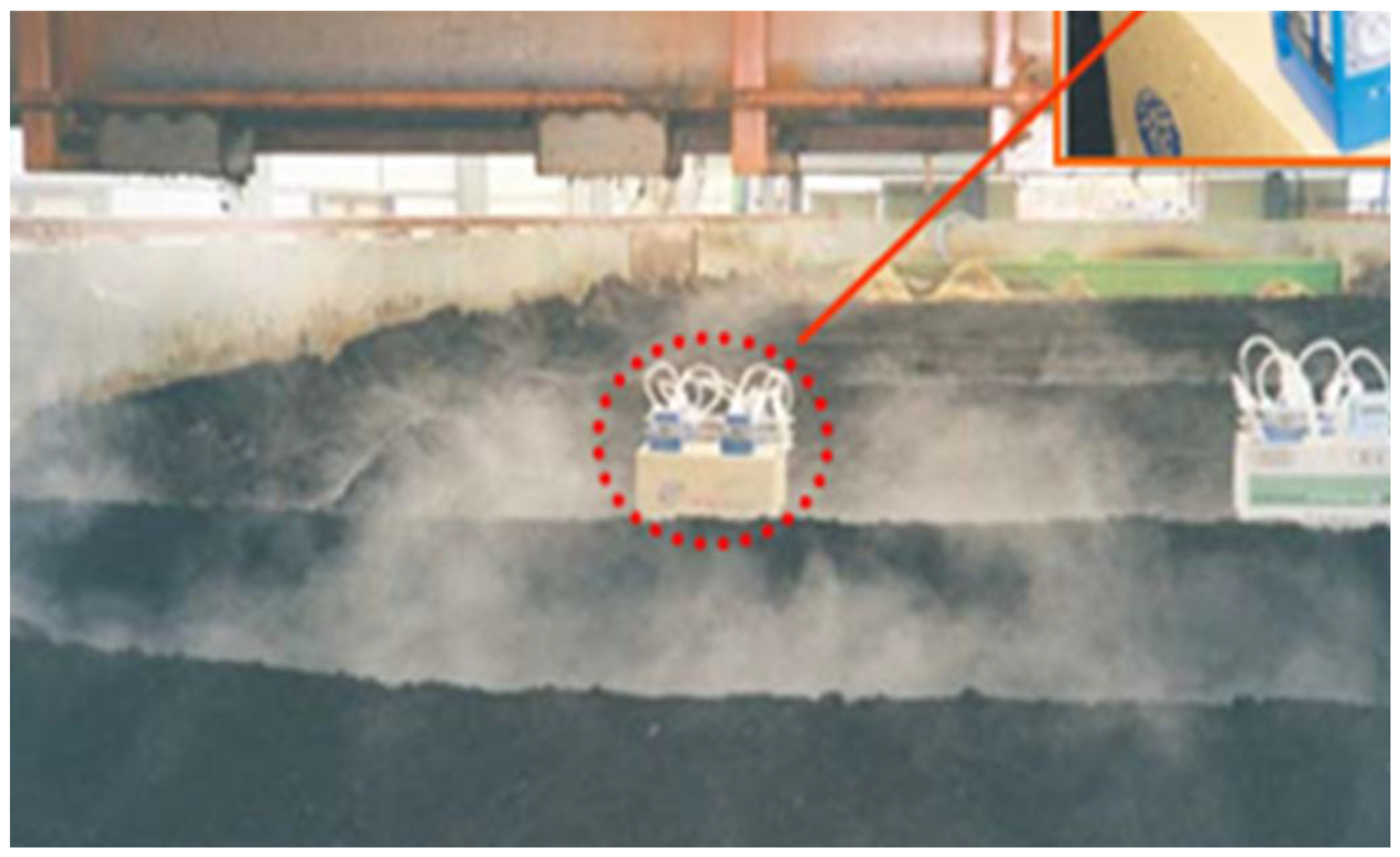
Figure 1 shows the method of measuring (direct measurement) the greenhouse gases CO₂ and methane through the gas detector tube at the composting (resource recovery) facility, where an escalator-type agitator mixes livestock excretions with sawdust and bulking agent.

Figure 2 presents the CO₂/methane gas collection operation for instrumental analysis at the composting facility using the escalator-type agitator, which mixes livestock excretions, sawdust, and bulking agent altogether.

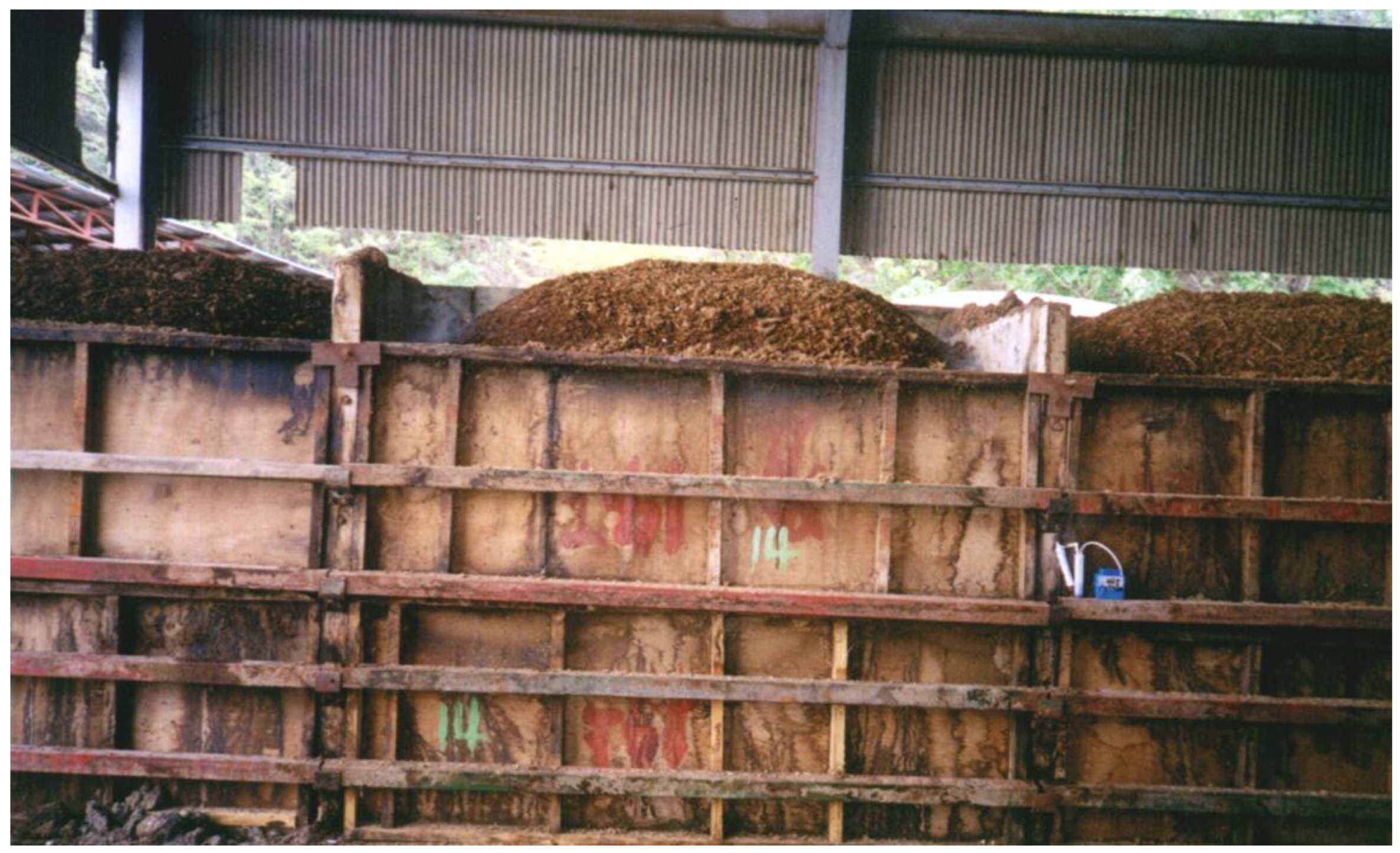
Figure 3 shows the CO₂/methane gas collection operation for instrumental analysis at the composting facility where livestock excretions, sawdust, and bulking agent are mixed together without any agitating operation (stacking method).

The GC-TCD analysis equipment used in this study to calculate the volume of carbon emissions generated during the pig-manure composting process is a thermal conductivity detector based on the principle of gas chromatography. It is very convenient and quite durable and sensitive, but has a low selectivity when analyzing samples, so is mostly used for analyzing gases.

As a method of analyzing the inorganic gases such as argon, nitrogen, hydrogen, and carbon dioxide or small CO₂ molecules, the TCD compares the thermal conductivities between the net transport gas and the sample gas. The temperature changes in the detector’s electric heating wire are affected by the conductivity of a gas flowing nearby and the change in conductivity is detected based on the changes in electric resistance, which is then used for measurement.

Meanwhile, water and oxygen cause some interactions at a stationary stage and create a high baseline noise in the emission gas chromatogram or generate a serious problem similar to a column elution, reducing the sensitivity of the detector and shortening the life of the column. In this regard, as with the other GC techniques, a transport gas with low concentration of water or oxygen impurities is required. Also, since the impurity of water or oxygen in a detection gas can cause oxidation of the detector wire, the TCD can be affected as well. Thus, using a compensating mixed-gas for calibrating the analyzer is a common practice.

3.1. Object

The selected farmhouse is raising 3000 growing pigs and 100 mother pigs in Mado-myeon, Hwaseong-si, Gyeonggi-do, Republic of Korea. The swine farm is of the sawdust-made, natural ventilation type. The farmhouse contains a screw-type agitating composting treatment facility with capacity of 330 m². About 6 tons/day of pig soil is discharged. The composting treatment period was for 8 days from 15:00 h, 28 October, to 11:00 h, 4 November. To compare the condition before and after mixing, the mixing was implemented after six days; two days later, the condition was measured as the after-the-mixing point. The soil was delivered to the composting treatment facility 10 days earlier, with about 60 tons put in storage. The mixing was implemented at 15:00 h on 2 November.

As for the research process, the inflow and discharge of gas (CO₂ and CH₄) in the swine farm composting treatment facility as well as the temperature and humidity were measured in time series, and the variations of the gas and temperature and humidity were investigated; peculiar aspects and results were recorded as well. To compare the condition before and after mixing, the gas and temperature and humidity were measured. A statistical technique—correlation analysis—was utilized to analyze the measurements, which were reflected in the results. The carbon emissions from the pig-manure composting treatment facility were calculated as the raw data.

3.2. Measurement

The composting treatment facility included the 330 m² mixing equipment with a steel roof and structure that is open to sunlight and air outside on part of the upper and lower sides and with an open inlet to discharge the treated soil. The polypropylene (PP) film used in tent-making was utilized to prevent the air outside from coming in, and two big sirocco fans were used to induce fresh air. The unit was designed to discharge the generated gases. The generated gas and temperature were measured and recorded in real time. For sealing the structure for gas sampling at the pig-manure composting treatment facility, the four sides except the roof were sealed with an opaque PP film. The total volume of the soil treatment facility was about 1100 m³, and a large-scale sirocco fan with capacity of 150 m³/min was installed to air it out once every 10 min. To discharge the generated gas, a sirocco fan of the same size was also installed. The flow of the two sirocco fans was adjusted by means of an inverter that would control the velocity.

Since the composting process that utilizes night soil and sawdust involves fluctuations in temperature during the maturing process, a four-channel temperature measuring system was adopted to check the gas emissions as temperature changed in the composting process. As for the temperature measuring probe, 4 sets of Pt 100 Ω were used, and the measuring unit was equipped with a transmitter (Tm4S, Autonic, Yangsan Korea) for online monitoring. With regard to the measuring points of the composting treatment facility, the spots for the temperature measurement of the fresh gas and supplied gas (T1) and temperature measurement of the outlet gas (T4) were selected. In addition, since the side is 35 m long, two temperature sensors were installed as deep as 60 cm at certain points of the rear part (T2) and front part (T3) with respect to the location of the fresh gas supply.

The fans of the monitoring system installed at the composting treatment facility were operated; 2 h later, the flow of fresh gas supply started to be adjusted by means of an inverter operating in the range of 100~150 m³/min. The flow of discharged air was adjusted in the range of 80~110 m³/min with the monitoring system in steady-state, and GC-TCD (iGC 7200, DS Science Korea, Gyeonggi-do, Korea) analysis was performed. To analyze the carbon dioxide concentration in the fresh gas and gas from the composting process through GC-TCD, the system was corrected and stabilized for two months.

At the fans where fresh gas was supplied after the gas sampling system was stabilized and at the connecting pipe of the sampling system, a 1/4” tube was used for collection at the rate of 5 L/min through the oil-less compressor, and the process was then analyzed with supply at the rate of 30 mL/min through GC-TCD. In the same manner, to collect fresh gas at the back of the discharge fan, GC-TCD analysis was performed. As for GC-TCD, the concentration of gases in the fresh air and the concentration of discharged gases were analyzed and recorded by computers using the automatic input device operating at intervals of 30 min. In the composting process, the gas emissions from immediately after soil mixing until remixing through the mixing unit were analyzed. Based on the concentration values of the analyzed gases, the flux (carbon emissions), which is the gas emissions per unit area (flux, mg/m²s), was calculated as in the following expression:

$$\mathrm{Flux}=\mathrm{Fowrate}\ast \frac{C \mathrm{output}-C \mathrm{input}}{\mathrm{Area}}\ast \frac{\mathrm{P}\ast \mathrm{M}}{\mathrm{R}\ast \mathrm{T}}$$

(1)

• Flow rate: m³/s
• C_output: concentration of chamber (ppm)
• C_input: concentration of fresh air (ppm)
• Area: area of chamber (m²)
• P: pressure (Pa = kg/(m·s²))
• M: molecular weight (kg/kmol)
• R: gas constant (J/kmol)
• T: absolute temperature (K)

The temperature of fresh gas and discharged gas was measured directly in front and at the back of the fan and recorded at intervals of 30 min. As for the temperature measurement during the composting process, two different measuring points including the 280 m² rectangle-shaped area were selected, since the steps taken in the composting process differed depending on the location. Of the two areas, the side of fresh air inflow was on the rear side where the composting process had been implemented since long ago, whereas the composting process started relatively later on the front side. To select the appropriate sampling points, the temperature was measured at the two zones, and the points of average temperature were selected. Since the temperature sensor was to be removed while the mixing unit was operated, the locations in the sampling system were marked so that the temperature could be measured at the same spots.

3.3. Data Analysis

As for the data of gases including concentration, temperature, and relative humidity, statistical analysis was performed using the data collected by means of IBM_SPSS_V20. To verify the correlation among the concentration, temperature, and relative humidity of the gases, the bivariate correlation analysis method was adopted.

4. Results and Discussion

4.1. Gas Measurements in the Composting Facility

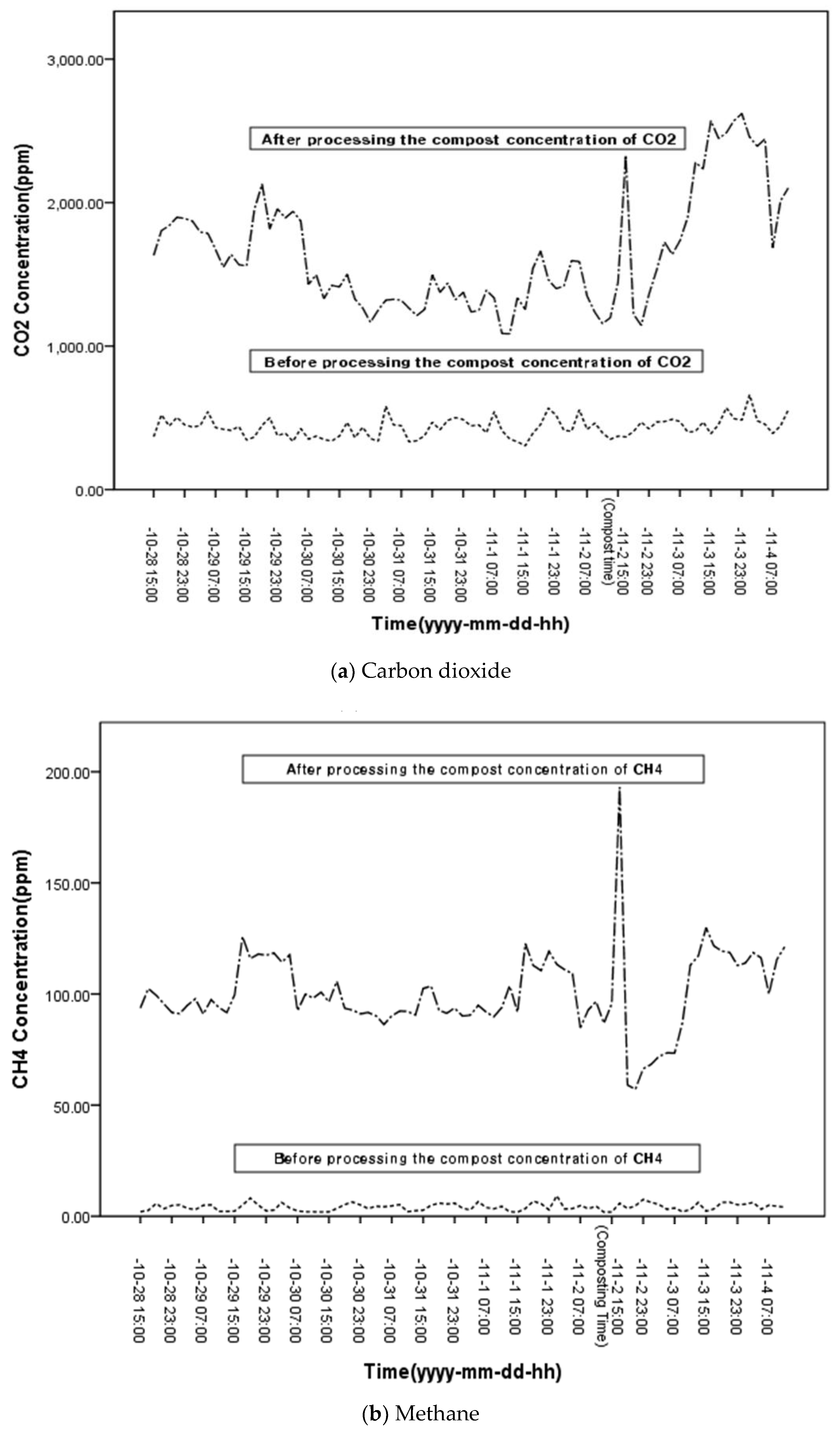
Figure 4 shows the distribution of carbon dioxide and methane in the air in a time series, measured in real time by the monitoring system during the composting process. In the air going through the composting process, the range of concentration of the generated carbon dioxide was 1086~2621 ppm, whereas that of the concentration of the generated carbon dioxide in the air outside the swine farm was 305~661 ppm, suggesting a major difference in distribution. This indicates that the condition of the night soil significantly affected the change in carbon dioxide emissions compared to the change in the air outside. The range of the generated methane concentration was 52~193 ppm, whereas that of the methane concentration in the air outside the swine farm was 2~9 ppm. This suggests a great difference in distribution compared to that of the air outside. Thus, the condition of night soil affected the changes in the amount of methane compared with that in the air outside.

Table 1. Carbon dioxide concentration and temperature according to process of the night soil treatment.

	CO2 after Soil Treatment (ppm)	CO2 before Soil Treatment (ppm)	CO2 during Soil Treatment (ppm)	Temperature of Intake Air (°C)	Temperature of Exhaust Air (°C)	Temperature in Front of the Farm (°C)	Temperature at the Back of the Farm (°C)
Mean	1642	434	1208	14.4	19.1	69.5	57.2
SD	402	69	385	4.2	5.3	3.4	5.5

presents the carbon dioxide concentration and temperature following soil treatment. After the process, CO₂ concentration was 1642 ± 402 ppm, whereas that in the air outside prior to the treatment was 434 ± 69 ppm. The CO₂ emission upon soil treatment was 1208 ± 385 ppm, and the intake and exhaust air temperatures were 14.4 ± 4.2 °C and 19.1 ± 5.3 °C, respectively. The temperature in front and at the back of the swine farm was 69.5 ± 3.4 °C and 57.2 ± 5.5 °C, respectively. The range of concentration was 673~2181 ppm, indicating that it exceeds the range of carbon dioxide concentration in the air outside, and that the composting condition consequently affects the range significantly.

Table 2. Methane concentration and temperature according to process of the night soil treatment.

	CH4 after Soil Treatment (ppm)	CH4 in Air before Soil Treatment (ppm)	CH4 during Soil Treatment (ppm)	Temperature of Intake Air (°C)	Temperature of Exhaust Air (°C)	Temperature in Front of the Farm (°C)	Temperature at the Back of the Farm (°C)
Mean	100	4	96	14.4	19.1	69.5	57.2
SD	18	2	18	4.2	5.3	3.4	5.5

shows the concentration and temperature of methane during the soil treatment. CH₄ concentration was 100 ± 18 ppm after the treatment, whereas that in the air outside was 4 ± 2 ppm prior to the treatment. The CH₄ emissions during the soil treatment were 96 ± 18 ppm. The intake air temperature and exhaust temperature were 14.4 ± 4.2 °C and 19.1 ± 5.3 °C, respectively, whereas the temperature in front and at the back of the swine farm was 69.5 ± 3.4 °C and 57.2 ± 5.5 °C, respectively.

4.2. Calculation of Carbon Dioxide and Methane Concentrations before and after Mixing

As for the composting process involved in the use of the mixing unit, the concentrations of carbon dioxide and methane differ before and after mixing. Thus, the carbon dioxide and methane emissions directly after mixing were measured, and the changes in their concentrations during and after the mixing process were observed.

Table 3. Carbon dioxide concentration and temperature according to process of soil treatment.

	CO2 after Soil Treatment (ppm)	CO2 before Soil Treatment (ppm)	CO2 during Soil Treatment (ppm)	Temperature of Intake Air (°C)	Temperature of Exhaust Air (°C)	Temperature in Front of the Farm (°C)	Temperature at the Back of the Farm (°C)
Before mixing
Mean	1498	423	1076	13.9	18.2	68.2	56.7
SD	256	67	251	4.2	5.3	2.4	6.0
After mixing
Mean	2040	465	1575	16.0	21.6	72.9	58.3
SD	468	67	456	3.9	4.3	3.4	3.6

presents the carbon dioxide concentration and temperature in soil treatment before and after the mixing process. Before the mixing process, CO₂ concentration after the treatment was 1498 ± 256 ppm, whereas that in the air outside prior to the soil treatment was 423 ± 67 ppm. The CO₂ emissions during the soil treatment were 1208 ± 385 ppm, and the intake and exhaust air temperatures were 13.9 ± 4.2 °C and 18.2 ± 5.3 °C, respectively. The temperature in front and at the back of the swine farm was 68.2 ± 2.4 °C and 56.7 ± 6.0 °C, respectively.

After the mixing process, the CO₂ concentration after treatment was 2040 ± 468 ppm, whereas that in the air prior to the treatment was 465 ± 67 ppm. The CO₂ emission during the soil treatment was 1575 ± 465 ppm, and the intake and exhaust air temperatures were 16.0 ± 3.9 °C and 21.6 ± 4.3 °C, respectively. The temperature in front and at the back of the farm was 72.9 ± 3.4 °C and 58.3 ± 3.6 °C, respectively, increasing by as much as 3.7 ± 1.0 °C and 1.6 ± 2.4 °C, respectively, after mixing. This suggests that the heat generated during the mixing process increased the temperature even outside the swine farm.

Table 4. Methane concentration and temperature according to process of soil treatment.

	CH4 after Soil Treatment (ppm)	CH4 in air before Soil Treatment (ppm)	CH4 during Soil Treatment (ppm)	Temperature of Intake Air (°C)	Temperature of Exhaust Air (°C)	Temperature. In Front of the Farm (°C)	Temperature in the Back of the Farm (°C)
Before mixing
Mean	99	4	95	13.9	18.2	68.2	56.7
SD	10	2	10	4.2	5.3	2.4	6.0
After mixing
Mean	103	5	98	16.0	21.6	72.9	58.3
SD	31	2	31	3.9	4.3	3.4	3.6

shows the methane concentration and temperature in the soil treatment before and after the mixing process. Before the mixing process, the CH₄ concentration after the treatment was 99 ± 10 ppm, whereas that in the air outside prior to the soil treatment was 4 ± 2 ppm. The CH₄ emissions during the treatment were 95 ± 10 ppm, and the intake and exhaust air temperatures were 13.9 ± 4.2 °C and 18.2 ± 5.3 °C, respectively. The temperature in front and at the back of the swine farm was 68.2 ± 2.4 °C and 56.7 ± 6.0 °C, respectively.

After the mixing process, the CH₄ concentration after treatment was 103 ± 31 ppm, and that in the air outside before treatment was 5 ± 2 ppm. The CH₄ emissions during the soil treatment were 98 ± 31 ppm, and the intake and exhaust air temperatures were 16.0 ± 3.9 °C and 21.6 ± 4.3 °C, respectively. The temperature in front and at the back of the swine farm was 72.9 ± 3.4 °C and 58.3 ± 3.6 °C, respectively, increasing by as much as 3.7 ± 1.0 °C and 1.6 ± 2.4 °C, respectively, after mixing. This indicates that the heat generated upon mixing increased the temperature even outside the farm.

Table 5. Concentration distribution of carbon dioxide and methane according to the composting process of swine manure.

		Minimum	Maximum	Mean	SD
CO2	During compost treatment	673	2181	1208	385
	Before compost turning	677	1682	1076	251
	After compost turning	673	2181	1575	456
CH4	During compost treatment	52	187	96	18
	Before compost turning	80	121	95	10
	After compost turning	52	187	98	31

presents the carbon dioxide and methane concentrations in treatment soil before and after mixing. The CO₂ concentration in the treatment was 1208 ± 385 ppm, 1076 ± 251 ppm before mixing, and 1575 ± 465 ppm after mixing, thus suggesting that CO₂ concentration increased after mixing. The CH₄ concentration in the soil treatment was 96 ± 18 ppm, 95 ± 10 ppm before mixing, and 98 ± 31 ppm after mixing. This indicates that CO₂ concentration increased after mixing. In conclusion, mixing affects the changes in CO₂ and CH₄ concentration to some extent.

4.3. Correlation between Carbon-Related Gases (Carbon Dioxide and Methane) and Environmental Factors

Table 6. Correlation relationship among comparative factors in the soil treatment during the swine manure mixing process.

	CO2 after Treatment	CO2 in the Outside Air before Treatment	CO2 in Treatment	CH4after Treatment	CH4 in the Outside Air before Treatment	CH4 in Treatment	Intake Air Temp.	Exhaust Air Temp.	Temp. in Front of the Farm	Temp. at the Back of the Farm
CO2 after treatment	1	0.327 **	0.986 **	0.611 **	0.176	0.599 **	0.132	−0.162	0.297 **	0.172
CO2 in the outside air before treatment		1	0.162	0.033	0.303 **	0.006	−0.297 **	−0.009	0.216 *	−0.311 **
CO2 in treatment			1	0.632 **	0.130	0.624 **	0.191	−0.168	0.272 *	0.235 *
CH4 after treatment				1	0.113	0.996 **	0.257 *	0.213	0.242 *	0.218 *
CH4 in the outside air before treatment					1	0.022	−0.386 **	0.083	0.178	−0.402 **
CH4 in treatment						1	0.294 **	0.207	0.227 *	0.256 *
Intake air temp.							1	0.210	0.251 *	0.978 **
Exhaust air temp.								1	0.785 **	0.158
Temp. in front of the farm									1	0.238 *
Temp. at the back of the farm										1

* <0.05, ** p < 0.01.

shows the result of analyzing the correlation among comparative factors in the soil treatment. The soil treatment and CO₂ emissions in the air outside the farm had a positive correlation, indicating that CO₂ concentration after the soil treatment affected the emission to a large extent. The temperature at various points around the swine farm showed a positive correlation, and the values were statistically significant. This suggests that since the temperature inside and outside the farm would affect the emissions, the temperature in the farm should be adjusted during extremely hot or cold seasons. In addition, the heat coming from the soil in the farm and the temperature outside the farm had a positive correlation, with values that were statistically significant, thus indicating that the heat generated from the soil was discharged to outside the swine farm. The amount of CO₂ in the air outside the farm, intake air temperature, and exhaust air temperature had a negative correlation with statistically significant values, and this has not been reported in existing documentation. Future studies are expected to conduct further research on this topic based on the findings above.

Table 7. Correlation Relationship among Comparative Factors in the Soil Treatment before and after the Swine Manure Mixing Process.

	CO2 after Treatment	CO2 in the Outside Air before Treatment	CO2 in Treatment	CH4 after Treatment	CH4 in the Outside Air before Treatment	CH4 in Treatment	Intake Air Temp.	Exhaust Air Temp.	Temp. in Front of the Farm	Temp. at the Back of the Farm
CO2 after treatment	1	0.252	0.990 **	0.791 **	−0.023	0.794 **	0.376	0.635 **	0.530 *	0.358
CO2 in the outside air before treatment		1	0.112	−0.045	0.290	−0.059	−0.156	0.199	0.367	−0.150
CO2 in treatment			1	0.819 **	−0.066	0.824 **	0.409	0.623 **	0.490 *	0.390
CH4 after treatment				1	0.062	0.999 **	0.521 *	0.748 **	0.428 *	0.458 *
CH4 in the outside air before treatment					1	0.014	−0.277	0.101	0.094	−0.307
CH4 in treatment						1	0.535*	0.745 **	0.424 *	0.474 *
Intake air temp.							1	0.296	0.184	0.975 **
Exhaust air temp.								1	0.880 **	0.185
Temp. in front of the farm									1	0.085
Temp. at the back of the farm										1

* <0.05, ** p < 0.01.

presents the correlation among comparative factors before and after mixing in the soil treatment. CO₂ emissions in the air outside the farm and soil treatment had a positive correlation, with values that were statistically significant both before and after mixing, thus suggesting that the mixing had an insignificant effect on the variations of CO₂ concentration. The amount of CO₂ in the air outside the farm before mixing had a negative correlation with the intake and exhaust air temperatures, whose values were statistically significant, although they were statistically insignificant after mixing. With regard to the air outside the farm, however, the CO₂ contents were believed to have changed temporarily due to environmental factors such as weather, not mixing. In addition, the correlation in terms of the change in temperature in front of the swine farm changed from a negative correlation to a positive one after mixing; such temperature change may be attributable to the changes in CO₂ content, but this needs to be verified through repeated experiments since there is no sufficient data on this.

4.4. Estimation of Carbon Emissions in the Discharged Gases

Among the pigs (6200/year) raised in the farm under the condition of 1 ha, 1 atm, and 291 ± 5.03 K during the year (365 days), the carbon emission from the night soil is calculated as follows:

The generated carbon dioxide was 2.023 ± 0.636 μg/h head, whereas the generation of carbon was 17.398 ± 5.467 g C/year head. The emissions of carbon dioxide and carbon before and after mixing are as follows: carbon dioxide before mixing was 1.810 ± 0.427 μg/h head, and carbon, 15.564 ± 3.671 g C/year head; carbon dioxide after mixing was 9.411 ± 2.692 g/h head, and carbon, 22.484 ± 6.431 ton C/year head.

Methane and carbon emissions were 0.059 ± 0.011 μg/h head and 1.385 ± 0.255 g C/year head, respectively. Methane and carbon emissions before and after mixing were as follows: methane before mixing was 0.058 ± 0.006 μg/h head, and carbon, 1.379 ± 0.147 g C/year head; methane after mixing was 0.059 ± 0.019 μg/h head, and carbon, 1.404 ± 0.439 g C/year head.

5. Conclusions

With the increased global interest in global warming, a multilateral effort to analyze the worldwide carbon balance to reduce carbon emissions is being made. The atmospheric CO₂ concentration is expected to rise from an average of 354 ppm in the 1990s to between 478 to 1099 in 2100 [21], and as a result, the earth-surface temperature is also expected to increase by 0.2 °C (2000) and 1.4 °C–5.8 °C by 2000 and 2100, respectively, largely affecting our lives. During the first stage of obligatory CO₂ reduction, the Republic of Korea was excluded from the nations who were obligated to reduce their CO₂ volume as it was classified as a developing country, but nevertheless, much effort is being made by the ROK to reduce its greenhouse gases.

The concentrations of CO₂ and methane, currently the main sources of atmospheric pollution, were analyzed during the pig-manure composting process in this study to understand and evaluate their effects.

For the amount of carbon dioxide in the composting process, the CO₂ concentration after the soil treatment was 1642 ± 402 ppm, whereas the content in the air outside was 434 ± 69 ppm. The CO₂ generated during the soil treatment was 1208 ± 385 ppm. The CO₂ concentration after the soil treatment was 2040 ± 468 ppm, whereas the content in the air before the treatment was 465 ± 67 ppm. The CO₂ generated from the soil treatment was 1575 ± 465 ppm. The temperature in front and at the back of the swine farm increased by as much as 3.7 ± 1.0 °C and 1.6 ± 2.4 °C, respectively, after mixing. In general, depending on the state of the night soil, changes in the amount of carbon dioxide were greater than those in the air outside, but the correlation analysis shows that the variations of CO₂ concentration did not result from the mixing process. Based on the results obtained from this study, the carbon emissions derived from carbon dioxide and methane emitted during the composting process of swine manure were estimated to be 15.564 ± 3.671 g C/year head and −1.379 ± 0.147 g C/year head, respectively.

Considering the results obtained from this study, the carbon emissions generated by pig production in Korea cannot be ignored in terms of the effort to prevent global warming. Therefore, in order to prevent global warming, it is urgent to establish effective measures to reduce the carbon emissions of the pig farming industry in Korea. In addition, from the perspective of Agriculture 4.0, it is necessary to establish smart farms that can monitor and manage carbon emissions in real time as soon as possible.

The studies associated with issues of carbon circulation and carbon balance in the ROK’s agriculture industry have been mainly conducted for the forests, so the equivalent studies for the livestock industry are very scarce. Thus, it is expected that the results obtained from this study will be quite useful as basic data when calculating the percentage of the livestock industry in establishing a domestic greenhouse gas emission inventory by each industrial sector.