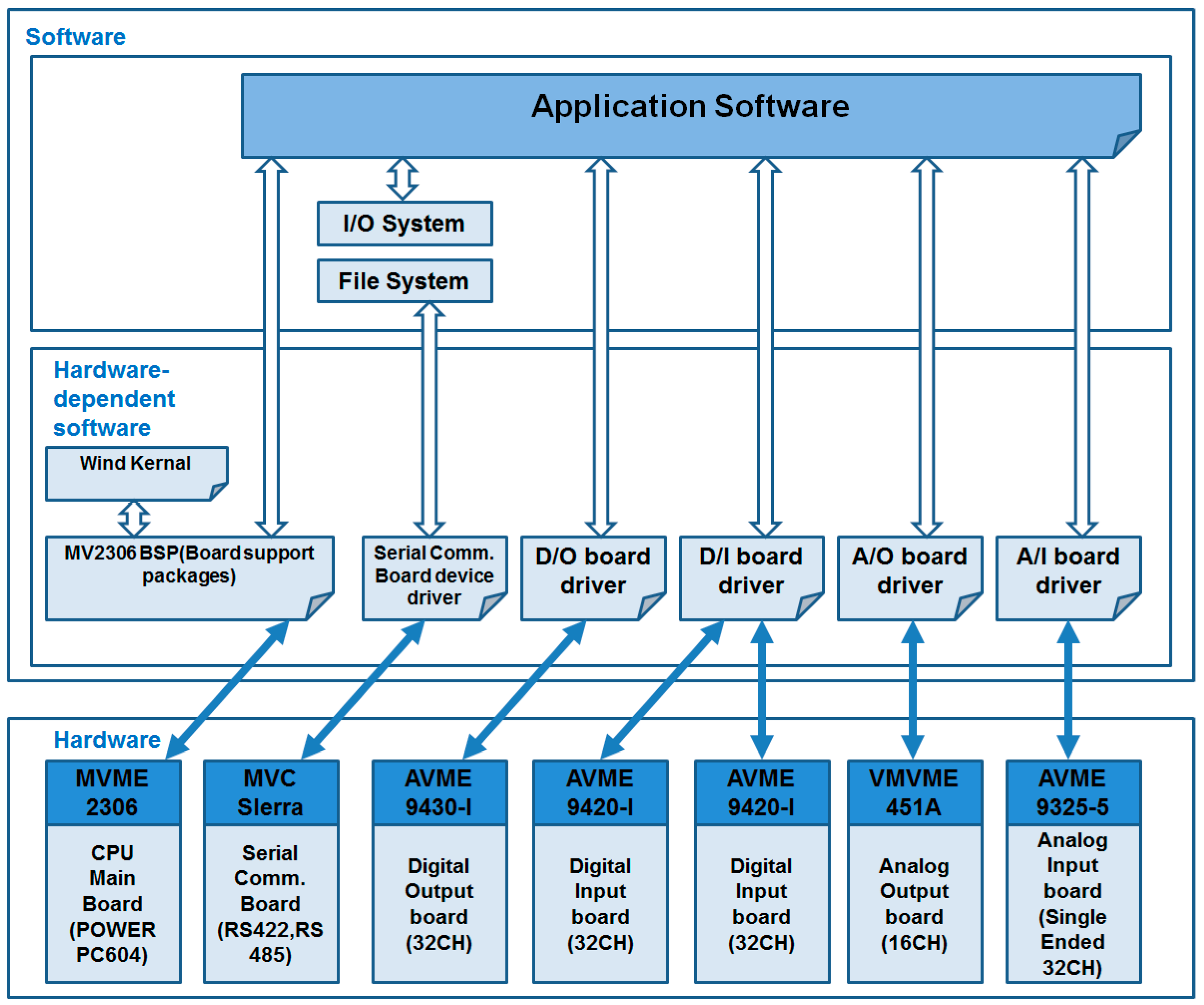
Figure 1.
Architecture of the Digital Excitation System.
Figure 1.
Architecture of the Digital Excitation System.
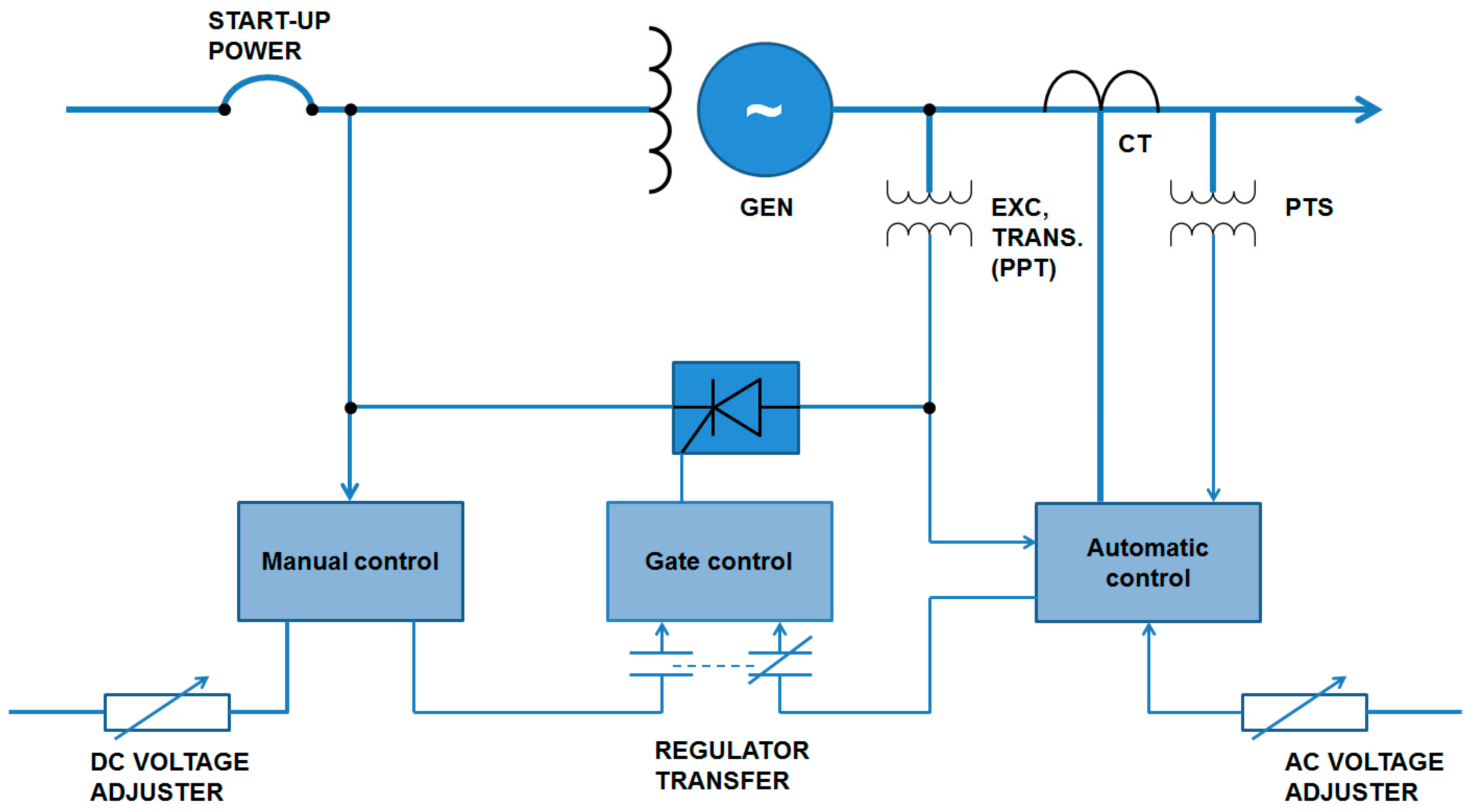
Figure 2.
Static Digital Excitation System Model.
Figure 2.
Static Digital Excitation System Model.
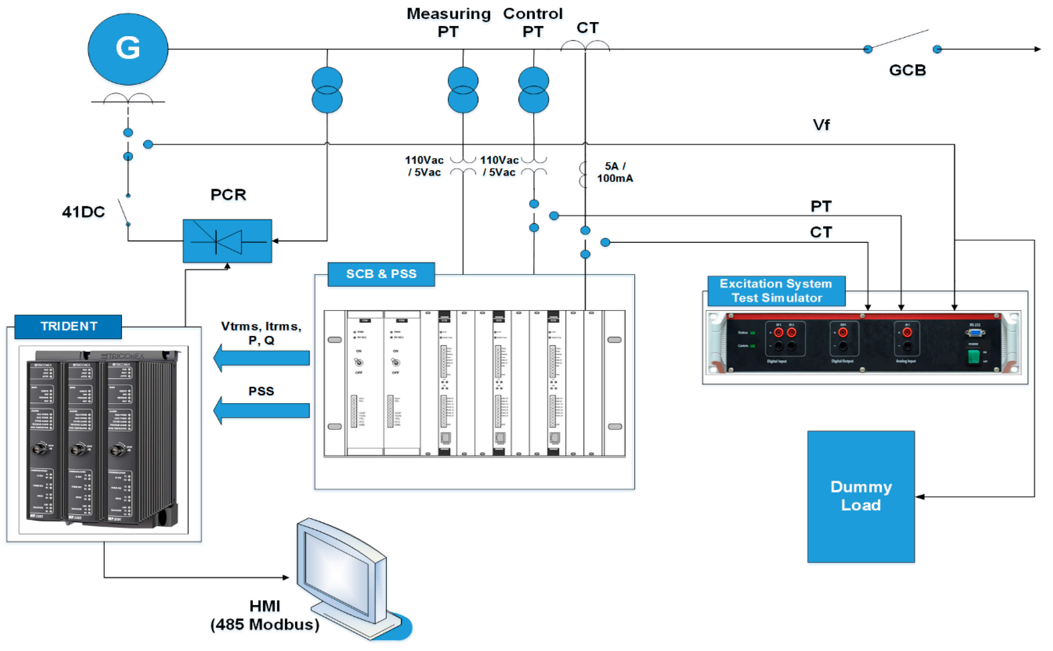
Figure 3.
Simulator-Mounted Redundant Digital Excitation System.
Figure 3.
Simulator-Mounted Redundant Digital Excitation System.
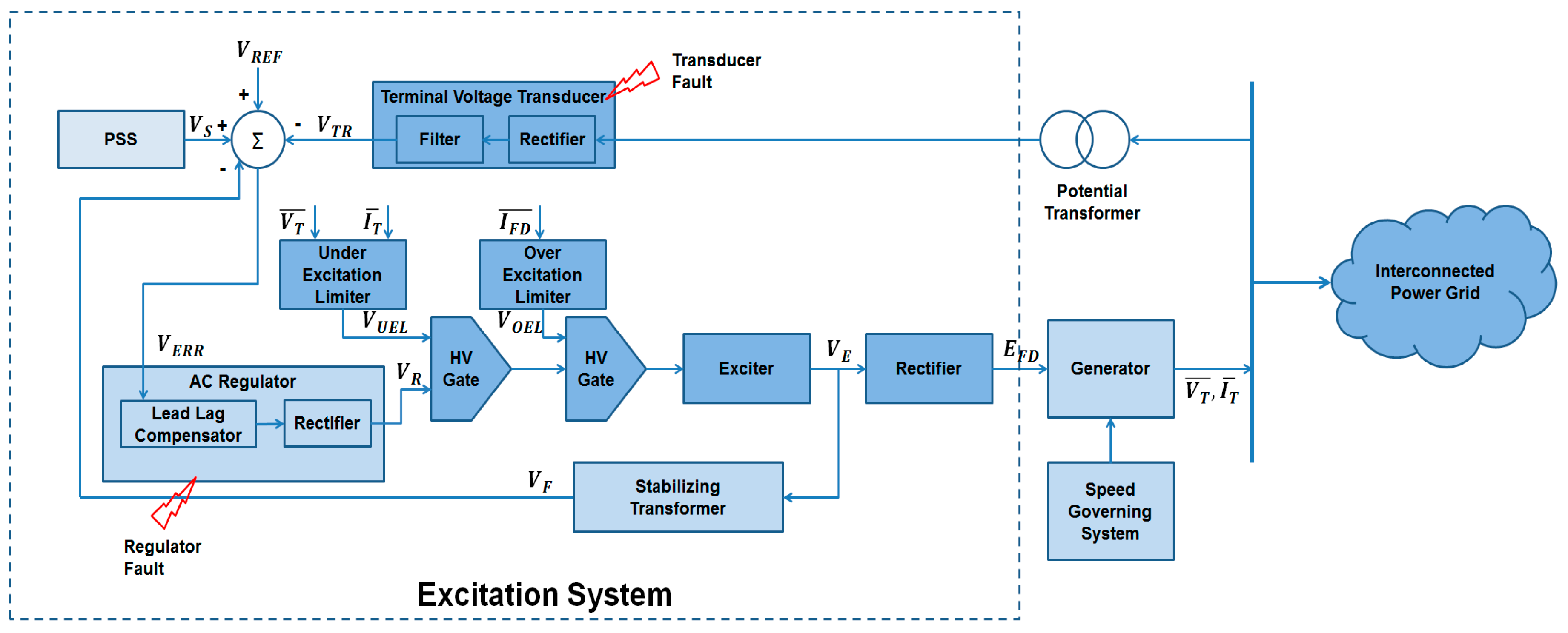
Figure 4.
Block Diagram of a Common Excitation System.
Figure 4.
Block Diagram of a Common Excitation System.
Figure 5.
Operating Times of the Digital Excitation System with Task Program.
Figure 5.
Operating Times of the Digital Excitation System with Task Program.
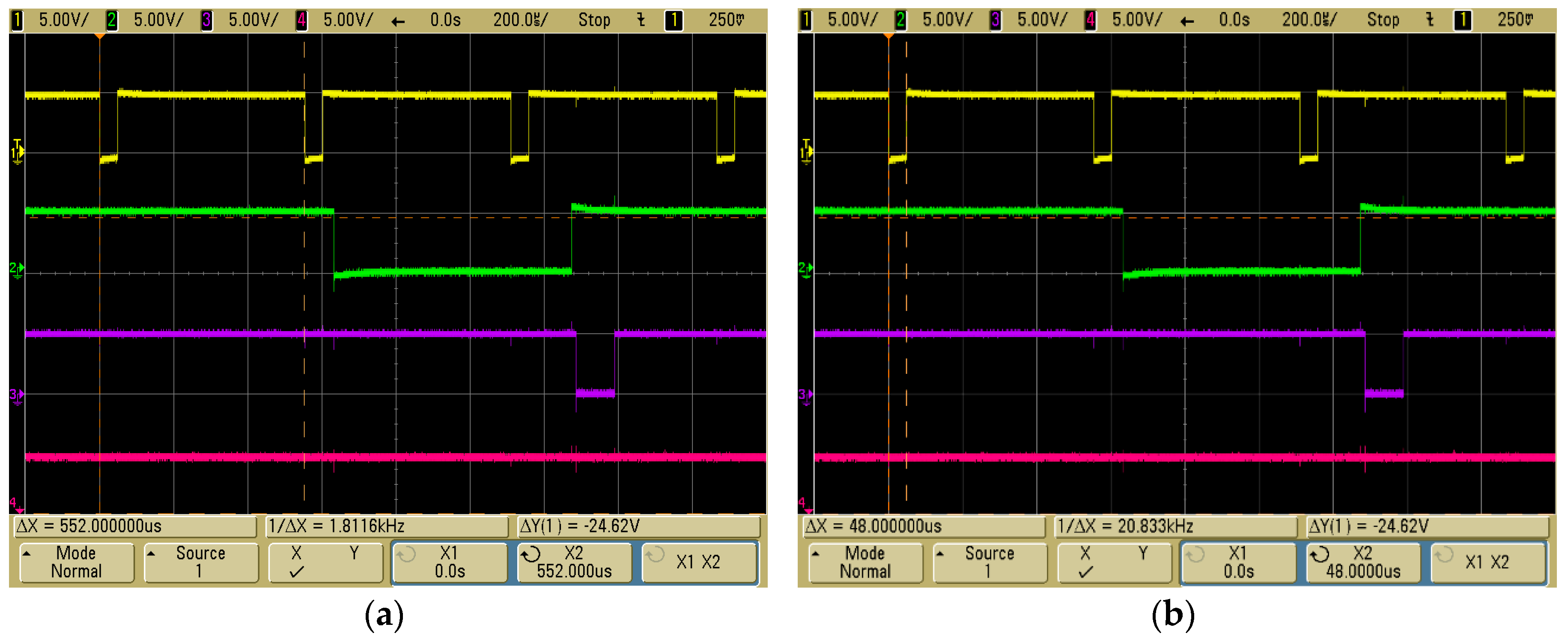
Figure 6.
Measurement of Excitation Control Program Operating Time ADC (Analog-Digital Converter). (a) ADC-based Sampling Cycle; (b) ADC-based Sampling Time.
Figure 6.
Measurement of Excitation Control Program Operating Time ADC (Analog-Digital Converter). (a) ADC-based Sampling Cycle; (b) ADC-based Sampling Time.
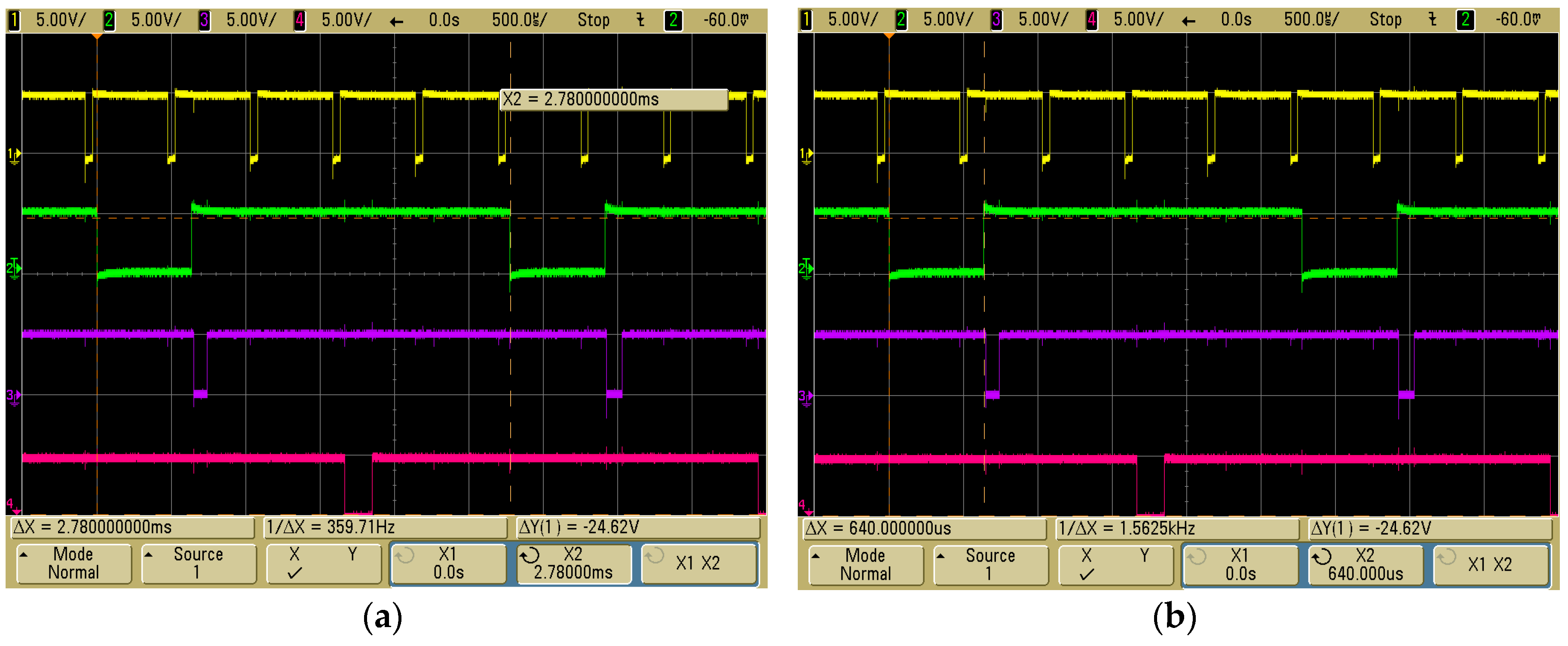
Figure 7.
DFT (Discrete Fourier Transform)—based Measurement of the Excitation Control Program. (a) DFT-based Sampling Cycle; (b) DFT-based Sampling Time.
Figure 7.
DFT (Discrete Fourier Transform)—based Measurement of the Excitation Control Program. (a) DFT-based Sampling Cycle; (b) DFT-based Sampling Time.
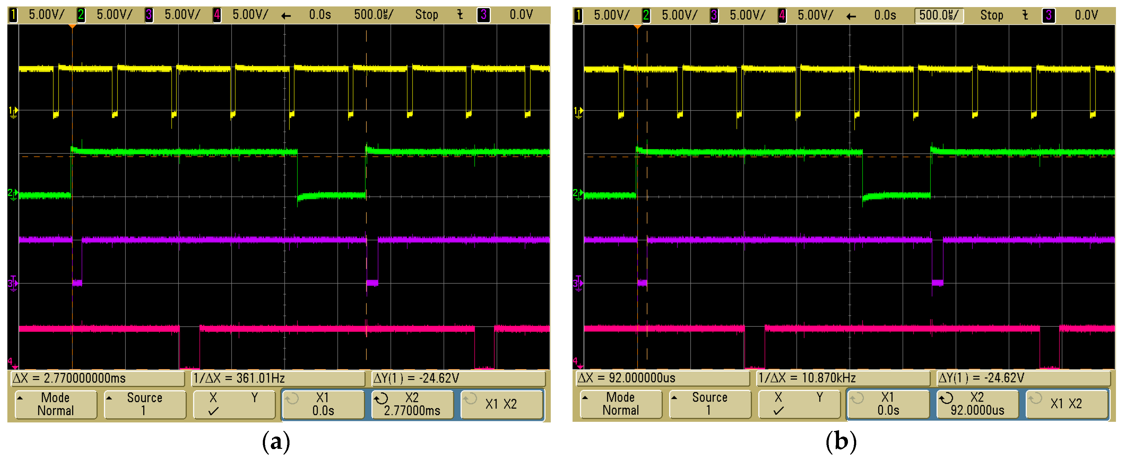
Figure 8.
Measurement of the Excitation Control Program Operation (Task). (a) Control Sampling Cycle (Task); (b) Control Sampling Time (Task).
Figure 8.
Measurement of the Excitation Control Program Operation (Task). (a) Control Sampling Cycle (Task); (b) Control Sampling Time (Task).
Figure 9.
Measurement of the Excitation Protection Program Operation (Task). (a) Protection Program Sampling Cycle (Task); (b) Protection Program Sampling Time (Task).
Figure 9.
Measurement of the Excitation Protection Program Operation (Task). (a) Protection Program Sampling Cycle (Task); (b) Protection Program Sampling Time (Task).
Figure 10.
Total Operating Time of the Programs.
Figure 10.
Total Operating Time of the Programs.
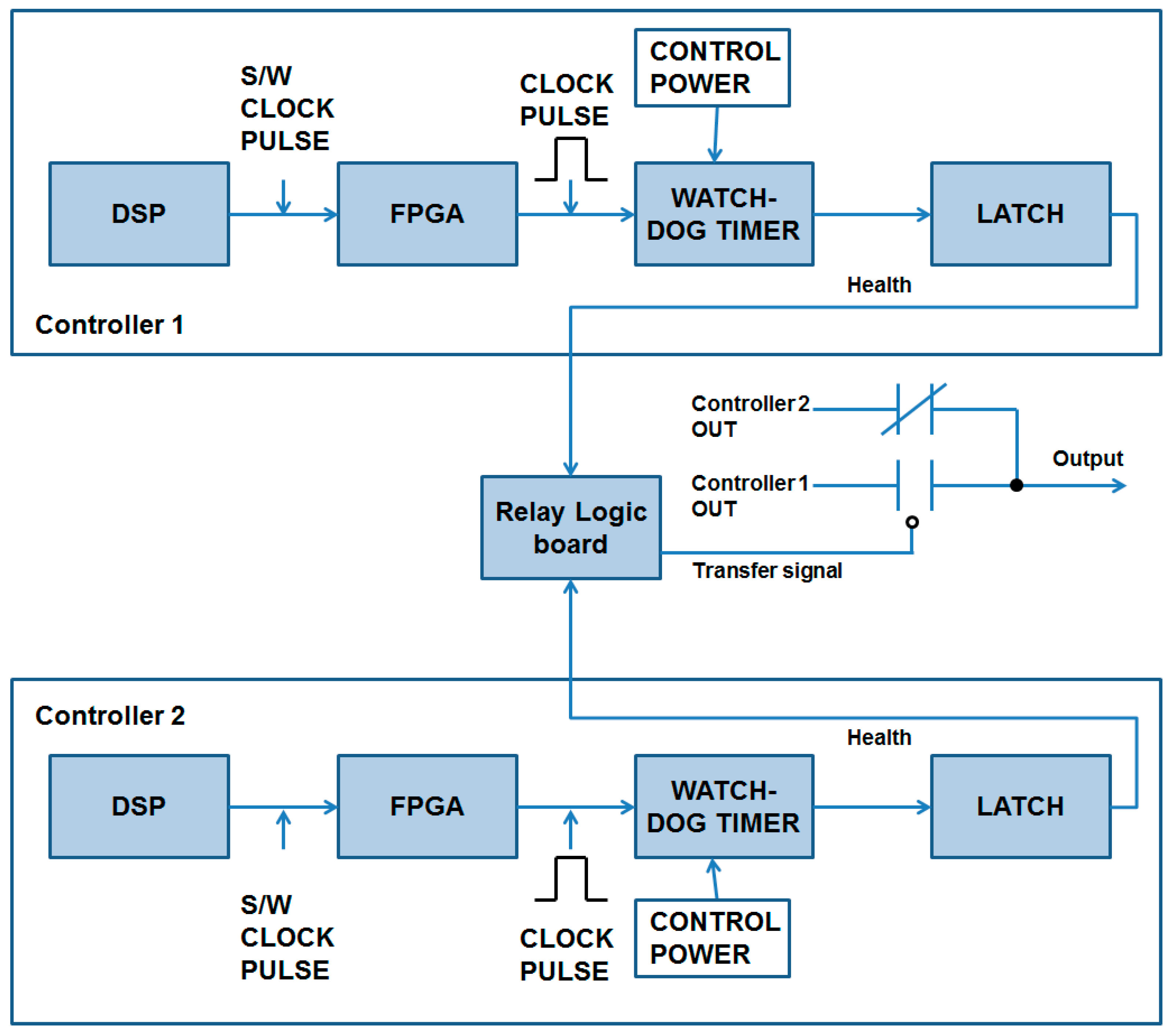
Figure 11.
Configuration of the Switchover Circuit of the Redundant Controller.
Figure 11.
Configuration of the Switchover Circuit of the Redundant Controller.
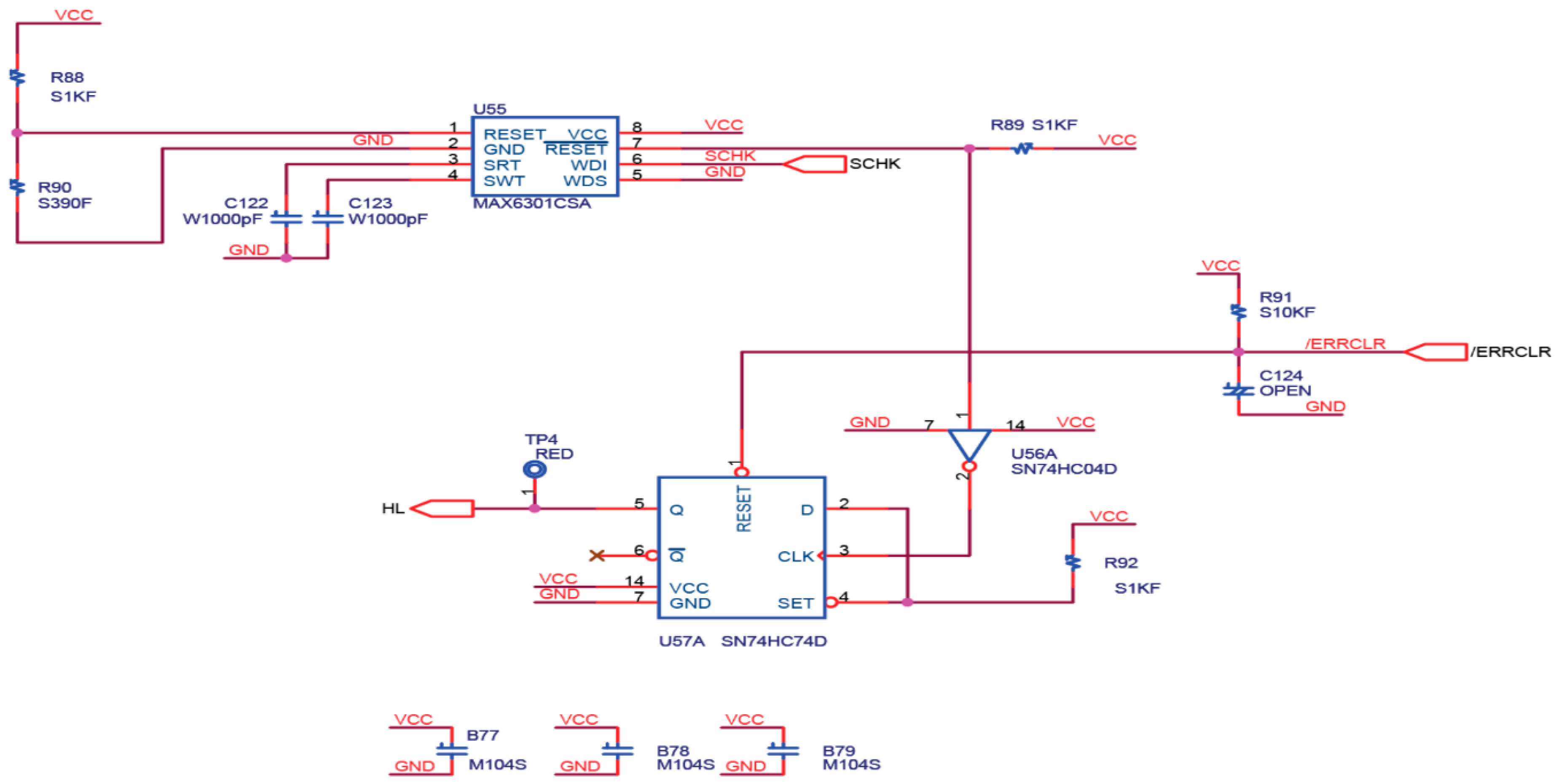
Figure 12.
Redundant Controller Switchover Circuit.
Figure 12.
Redundant Controller Switchover Circuit.
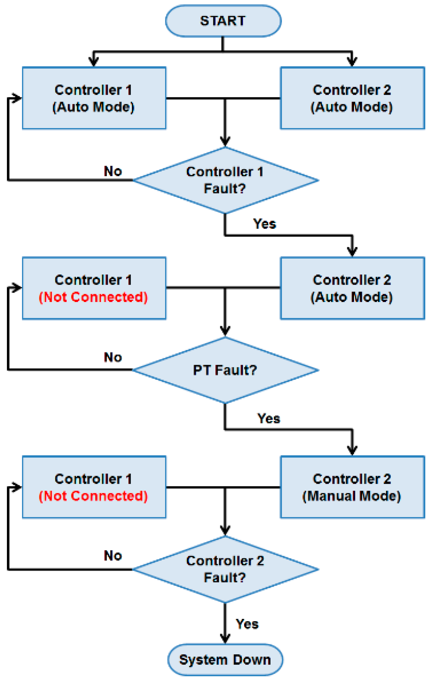
Figure 13.
Diagnosis Sequence of Redundant Controller Operating Mode.
Figure 13.
Diagnosis Sequence of Redundant Controller Operating Mode.
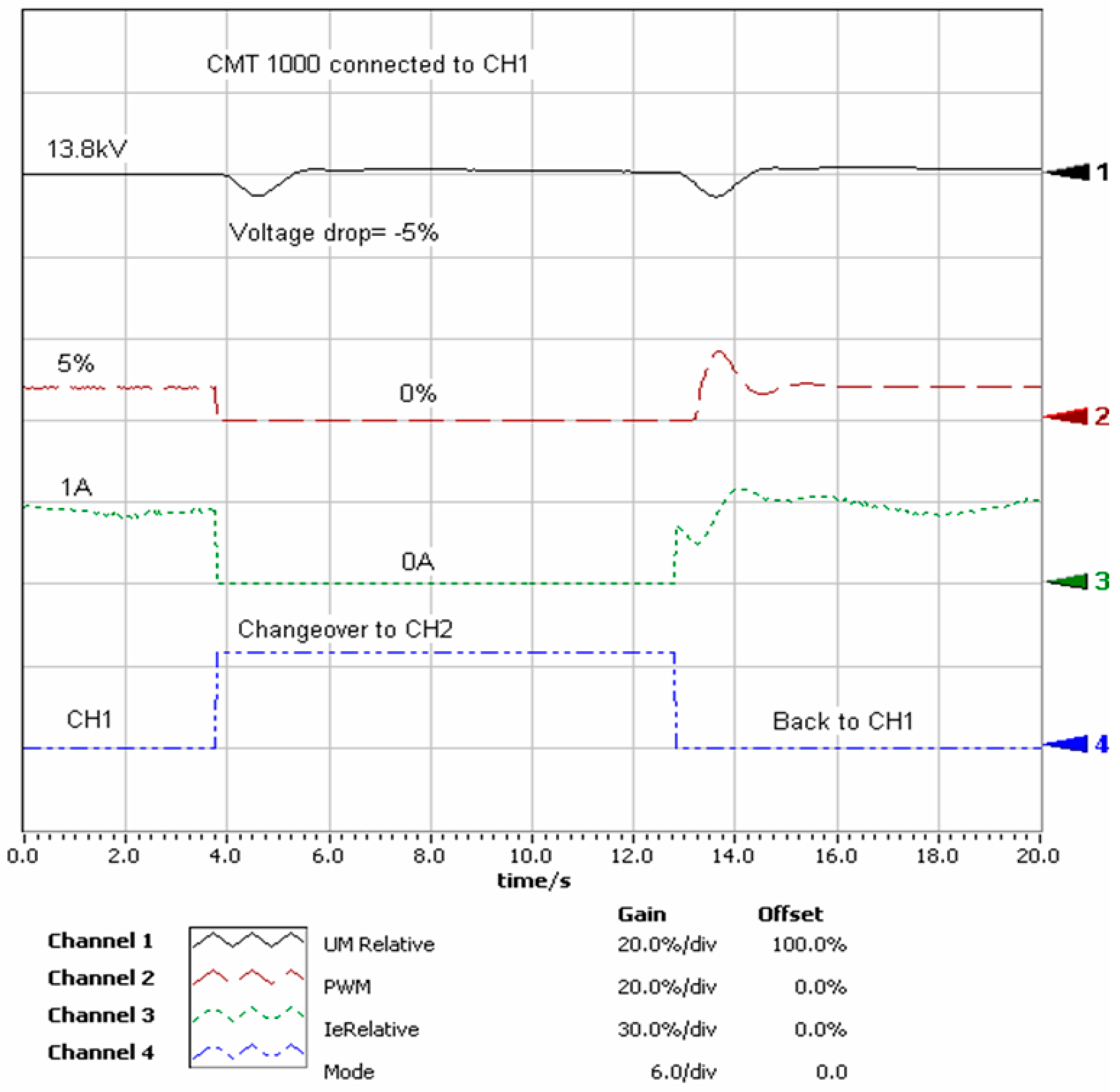
Figure 14.
Controller Switchover Test (Company A).
Figure 14.
Controller Switchover Test (Company A).
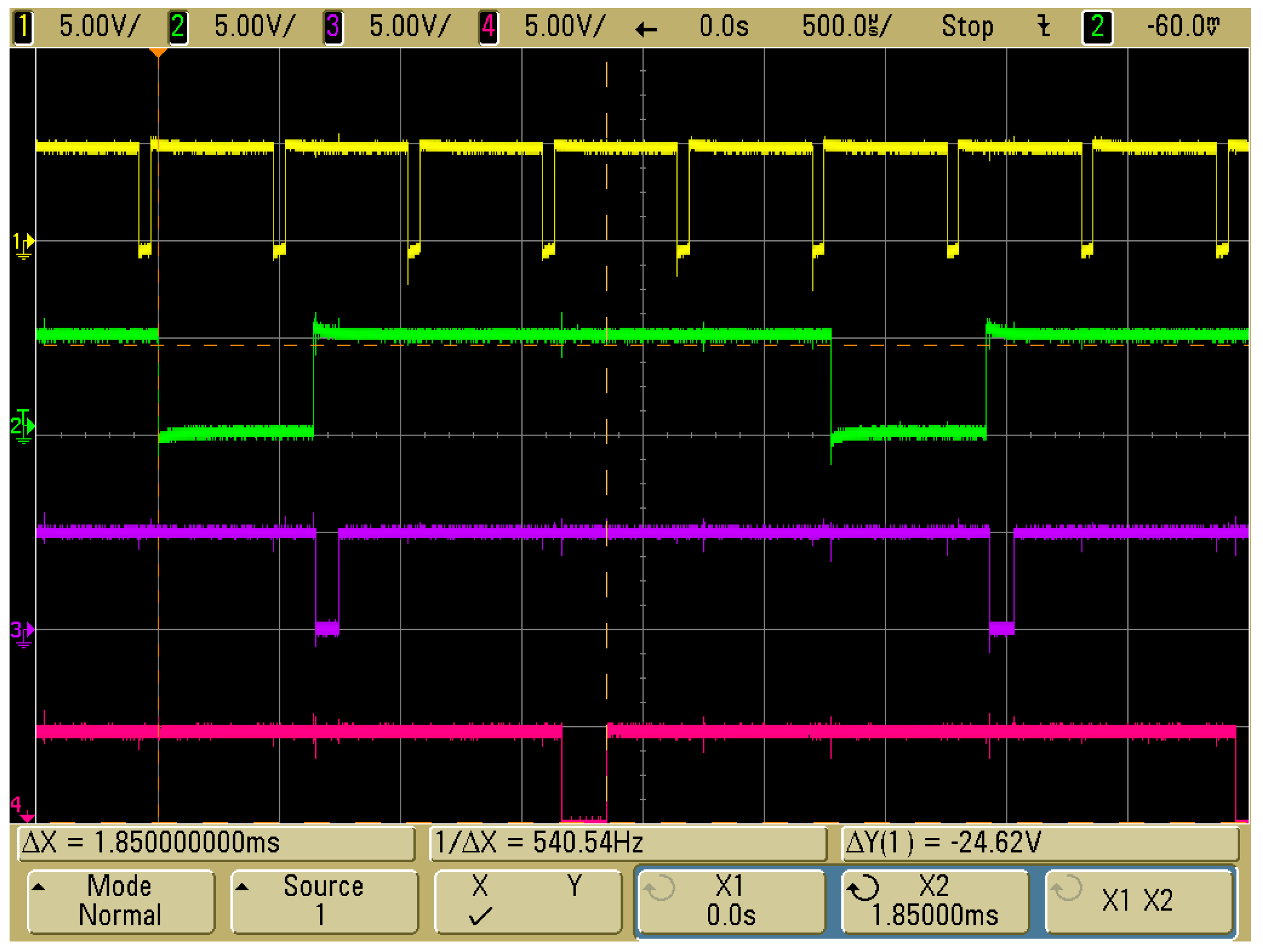
Figure 15.
Controller Switchover Test (Company B).
Figure 15.
Controller Switchover Test (Company B).
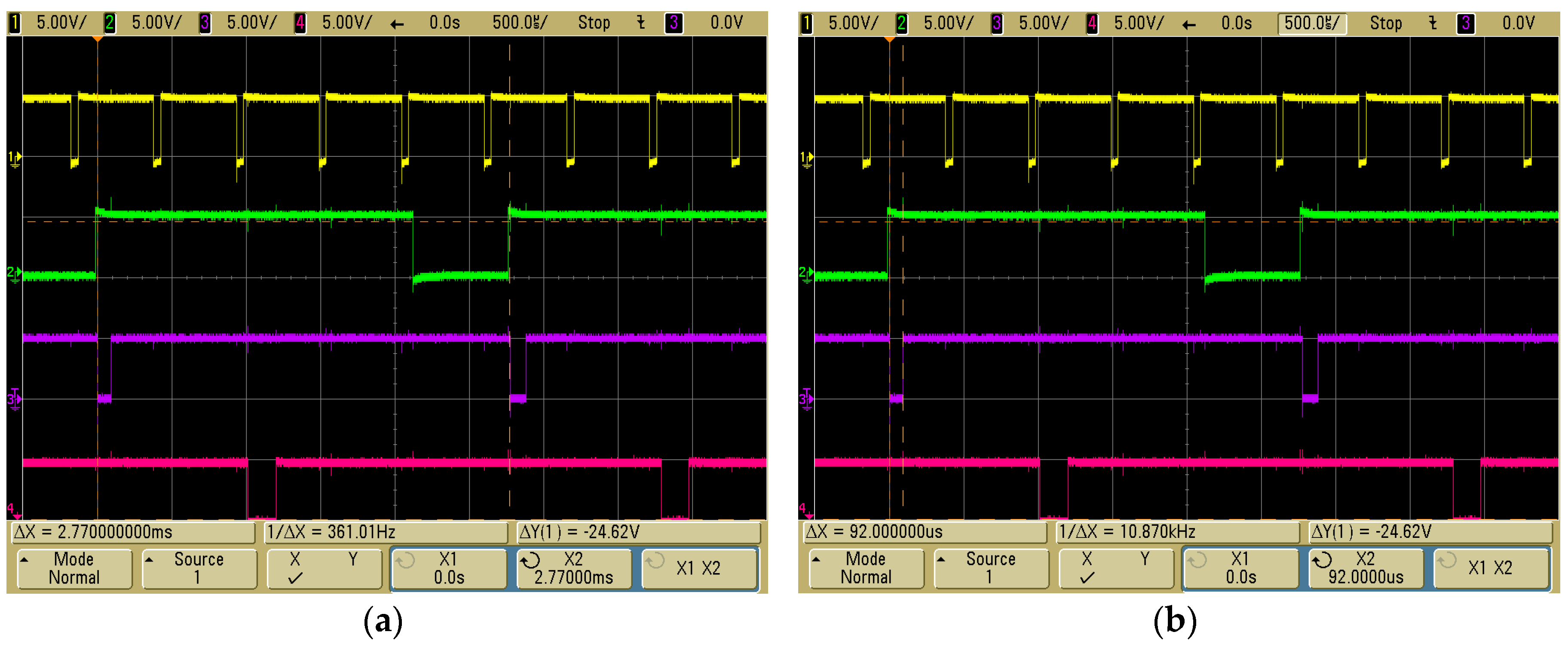
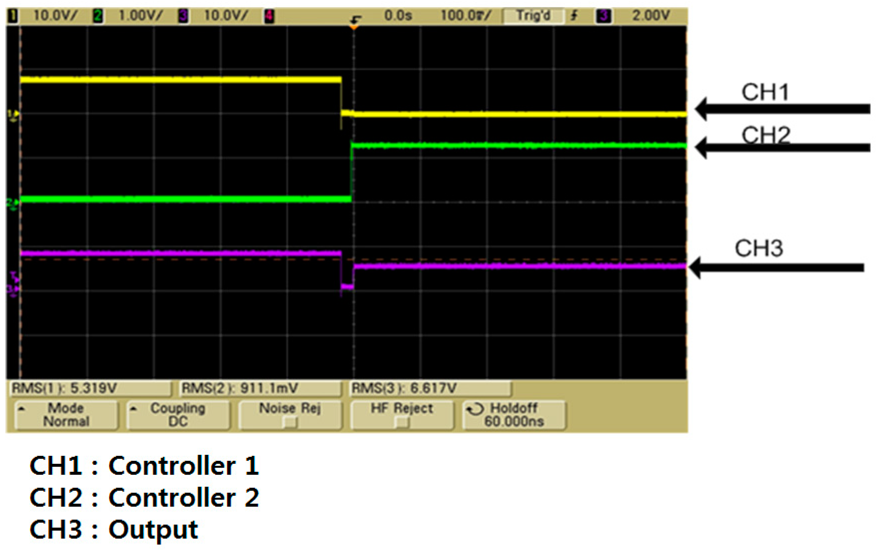
Figure 16.
Switchover Test of Redundant Controllers.
Figure 16.
Switchover Test of Redundant Controllers.
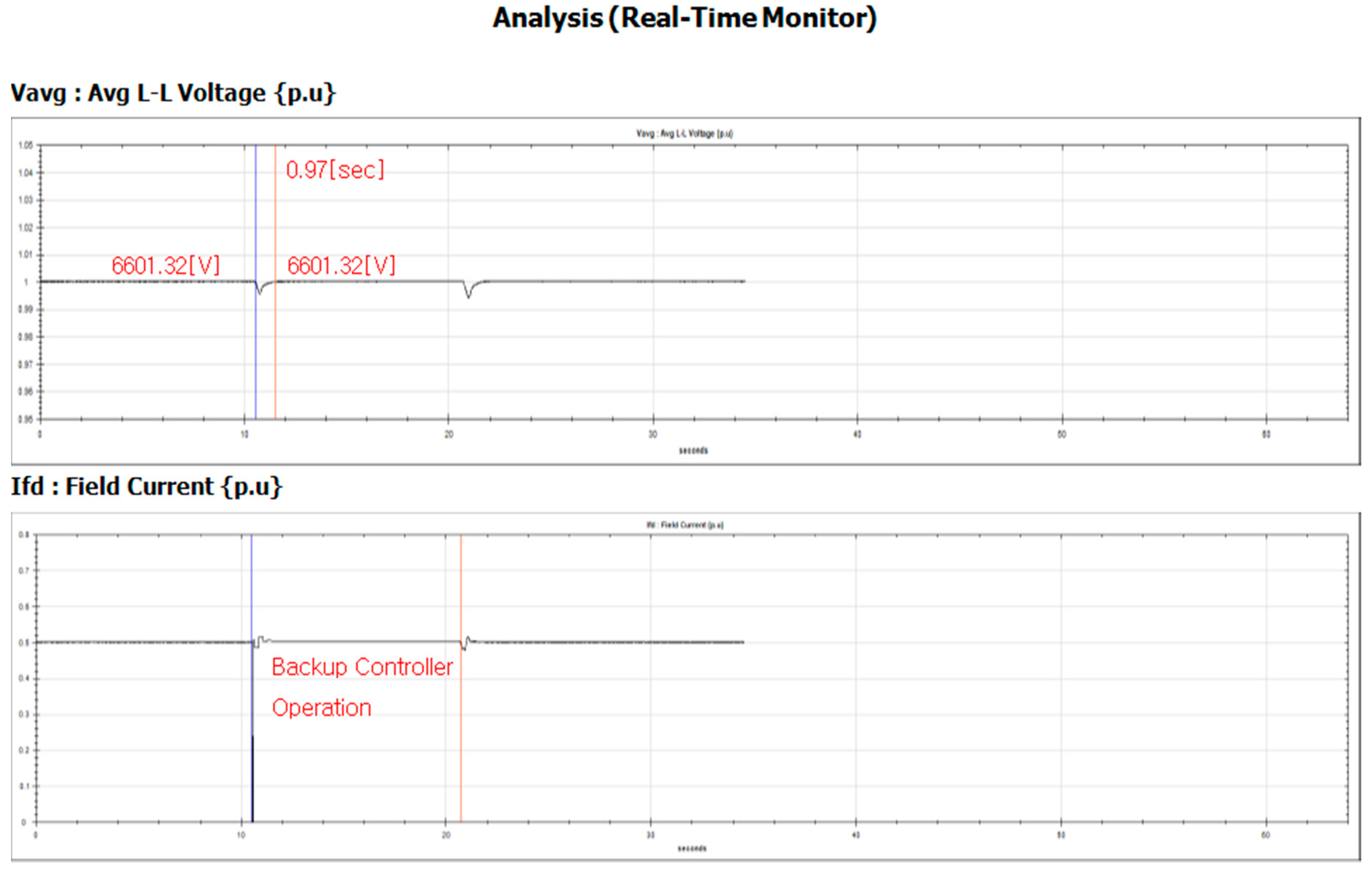
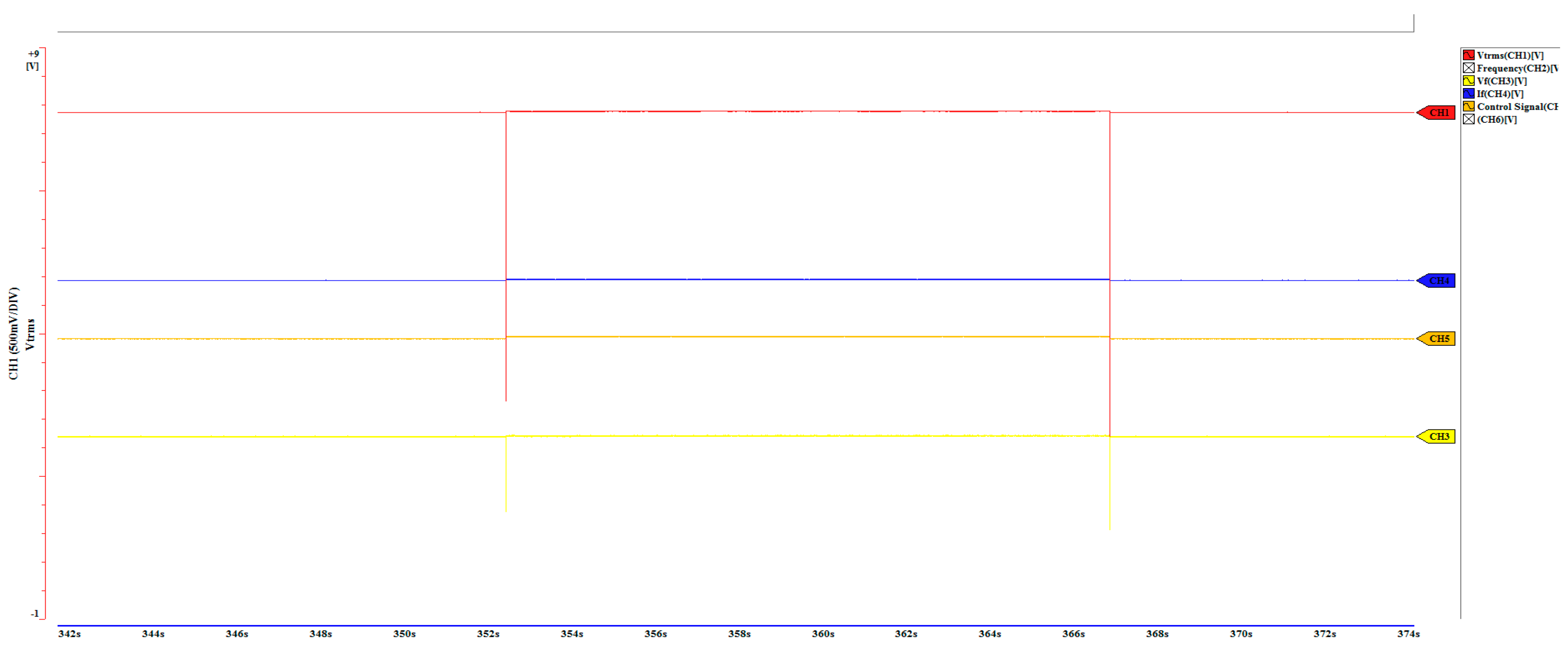
Figure 17.
Redundant Controller Switchover at the Field Test.
Figure 17.
Redundant Controller Switchover at the Field Test.
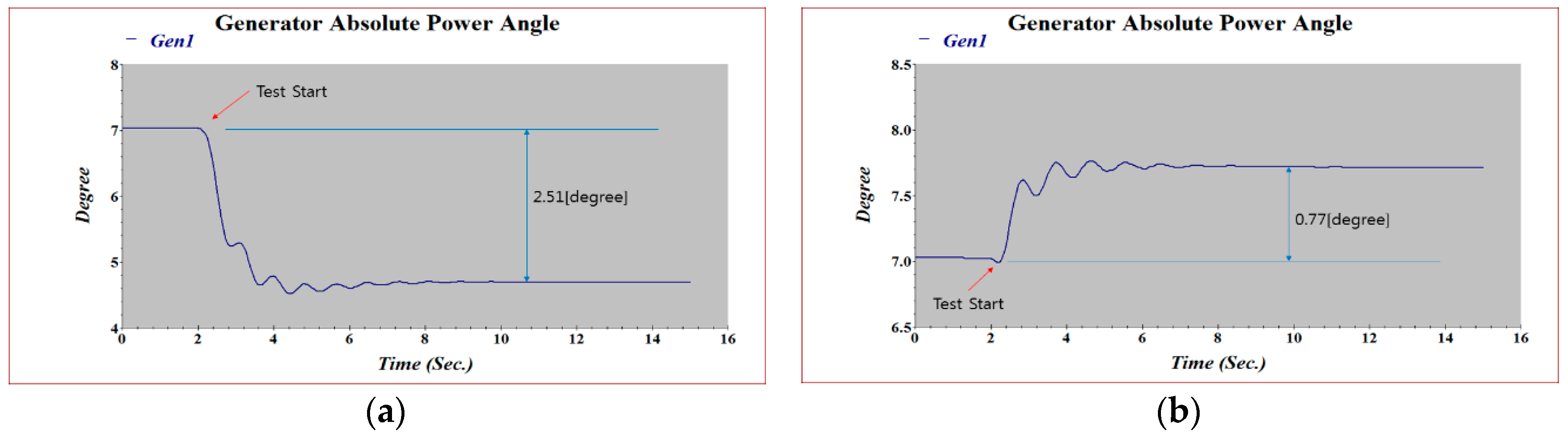
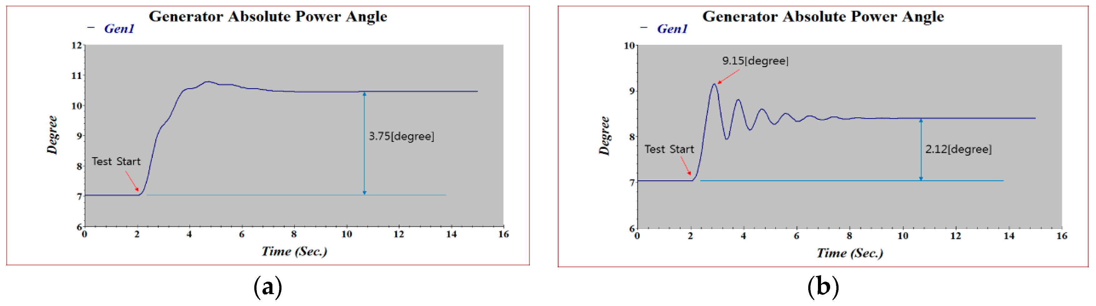
Figure 18.
Generator Power Phase Angles with/without OEL. (a) Without OEL at −10% Impact in Grid; (b) With OEL at −10% Impact in Grid.
Figure 18.
Generator Power Phase Angles with/without OEL. (a) Without OEL at −10% Impact in Grid; (b) With OEL at −10% Impact in Grid.
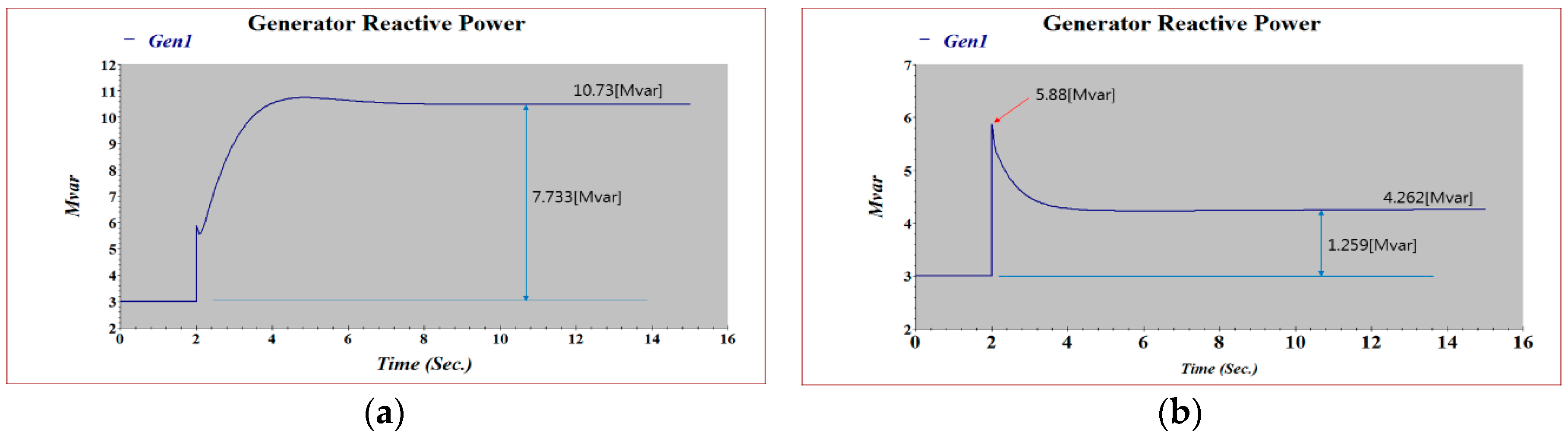
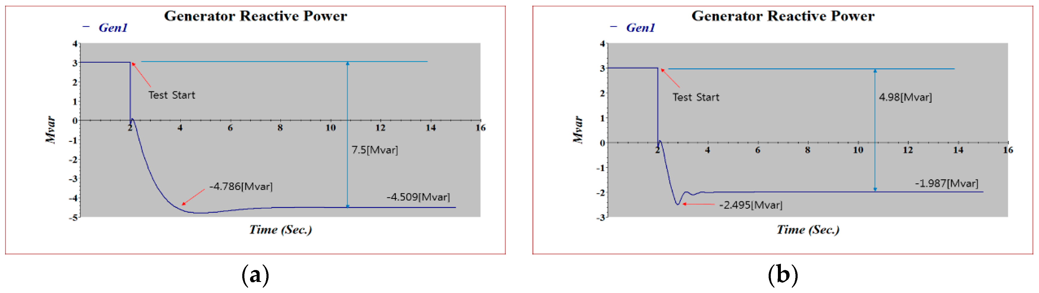
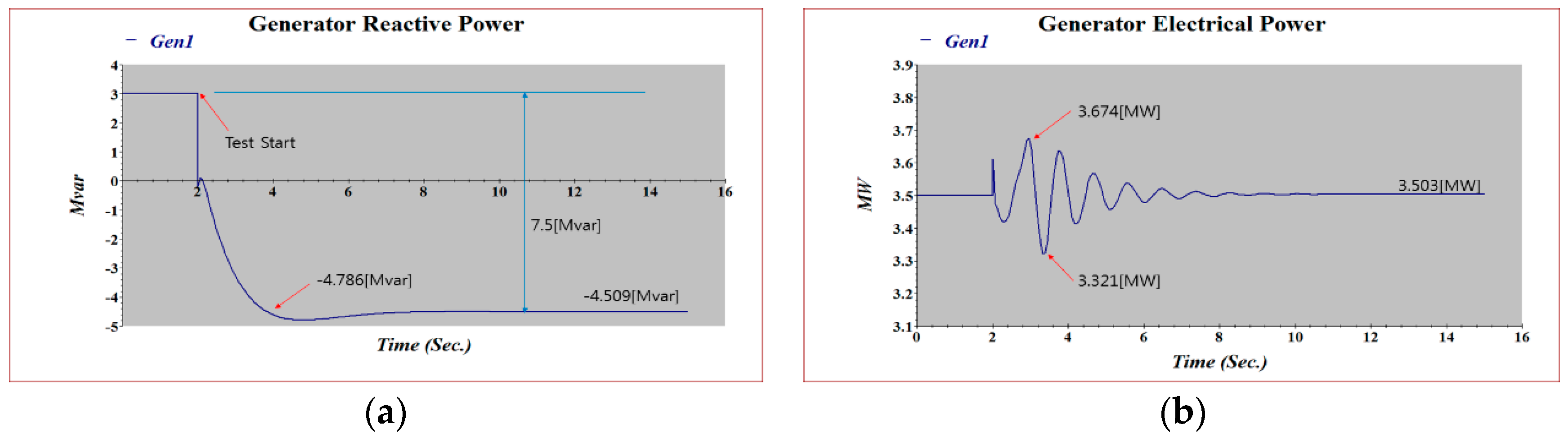
Figure 19.
Generator Reactive Power with/without OEL. (a) Without OEL at −10% Impact in Grid; (b) With OEL at −10% Impact in Grid.
Figure 19.
Generator Reactive Power with/without OEL. (a) Without OEL at −10% Impact in Grid; (b) With OEL at −10% Impact in Grid.
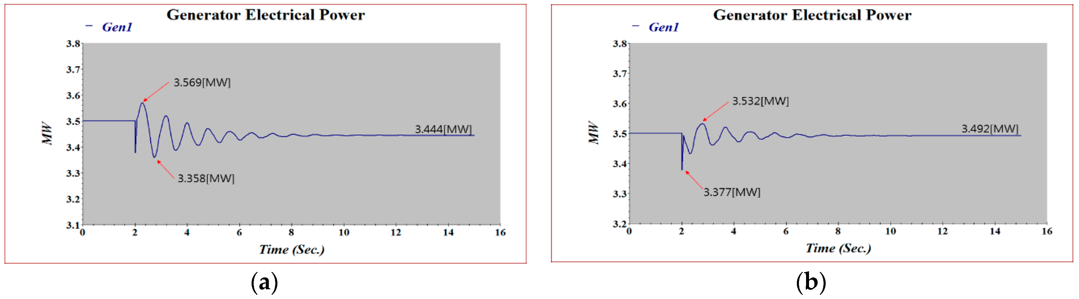
Figure 20.
Generator’s Active Power with/without Over Excitation Limiter (OEL). (a) Without OEL at −10% Impact in Grid; (b) With OEL at −10% Impact in Grid.
Figure 20.
Generator’s Active Power with/without Over Excitation Limiter (OEL). (a) Without OEL at −10% Impact in Grid; (b) With OEL at −10% Impact in Grid.
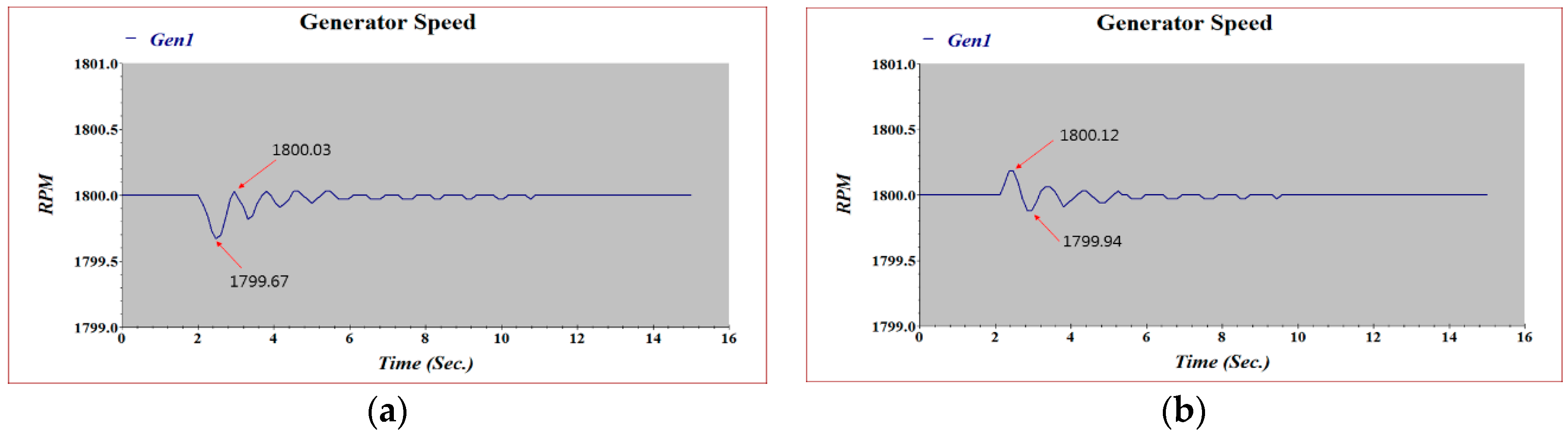
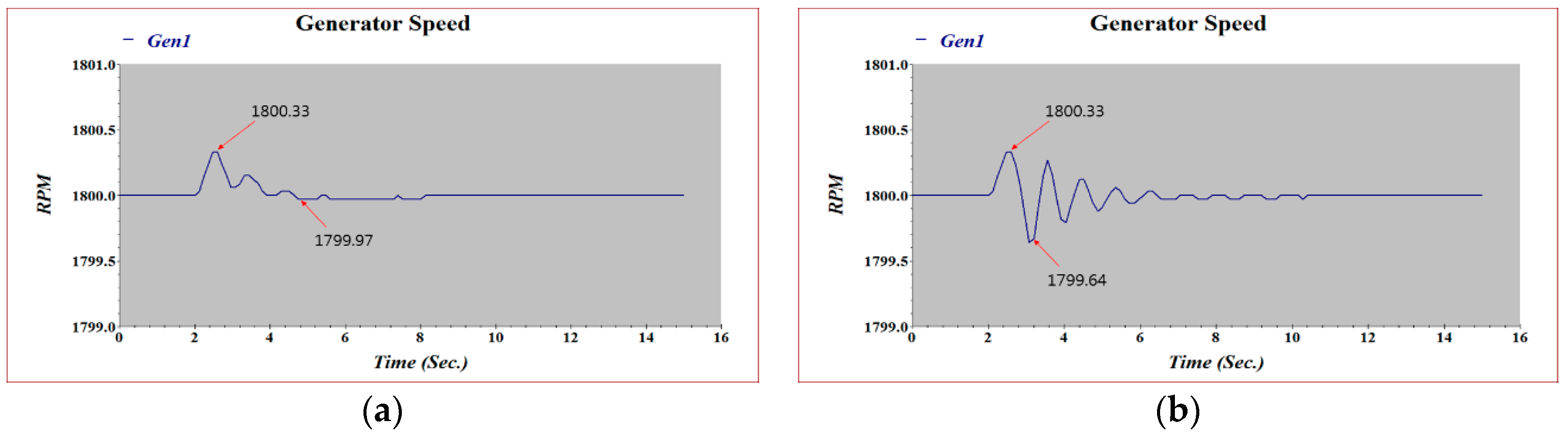
Figure 21.
Generator Speed with/without OEL. (a) Without OEL at −10% Impact in Grid; (b) With OEL at −10% Impact in Grid.
Figure 21.
Generator Speed with/without OEL. (a) Without OEL at −10% Impact in Grid; (b) With OEL at −10% Impact in Grid.
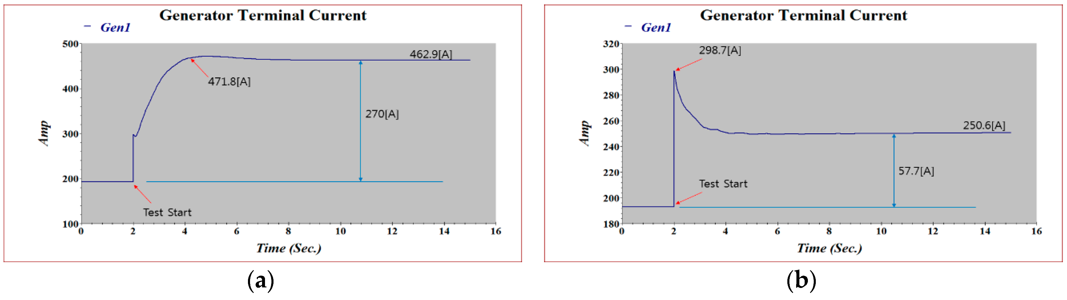
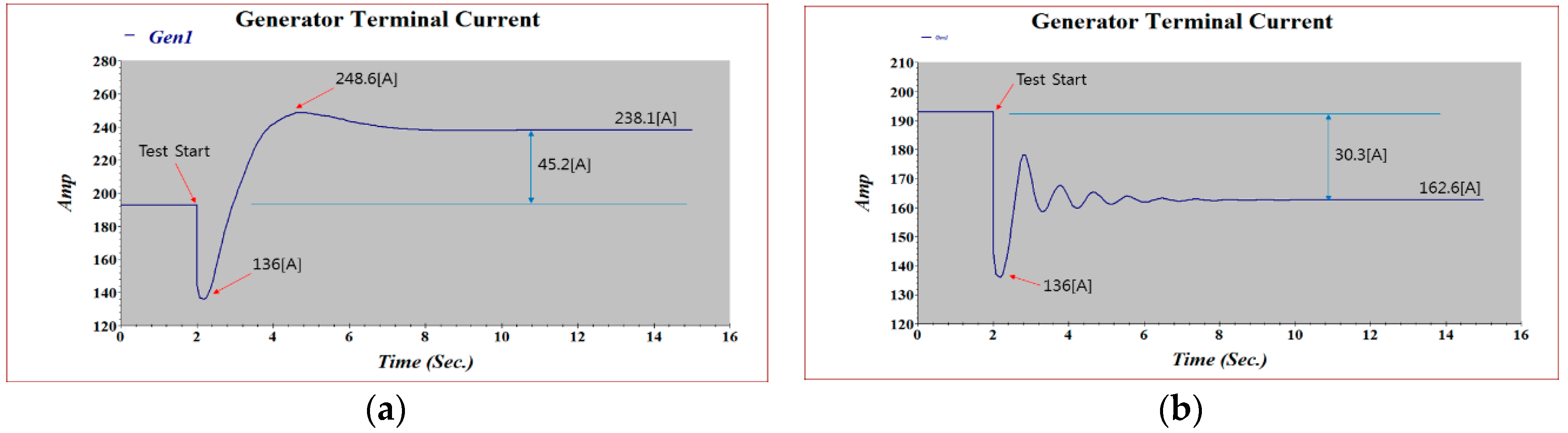
Figure 22.
Generator Current with/without OEL Function. (a) Without OEL at −10% Impact in Grid; (b) With OEL at −10% Impact in Grid.
Figure 22.
Generator Current with/without OEL Function. (a) Without OEL at −10% Impact in Grid; (b) With OEL at −10% Impact in Grid.
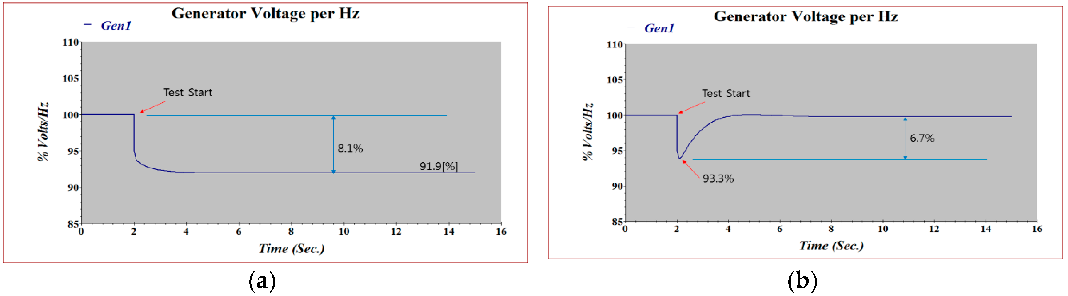
Figure 23.
Generator V/Hz with/without OEL Function. (a) Without OEL at −10% Impact in Grid; (b) With OEL at −10% Impact in Grid.
Figure 23.
Generator V/Hz with/without OEL Function. (a) Without OEL at −10% Impact in Grid; (b) With OEL at −10% Impact in Grid.
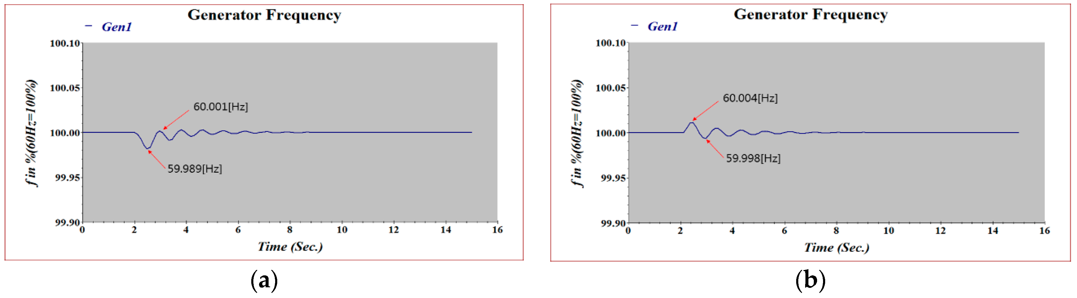
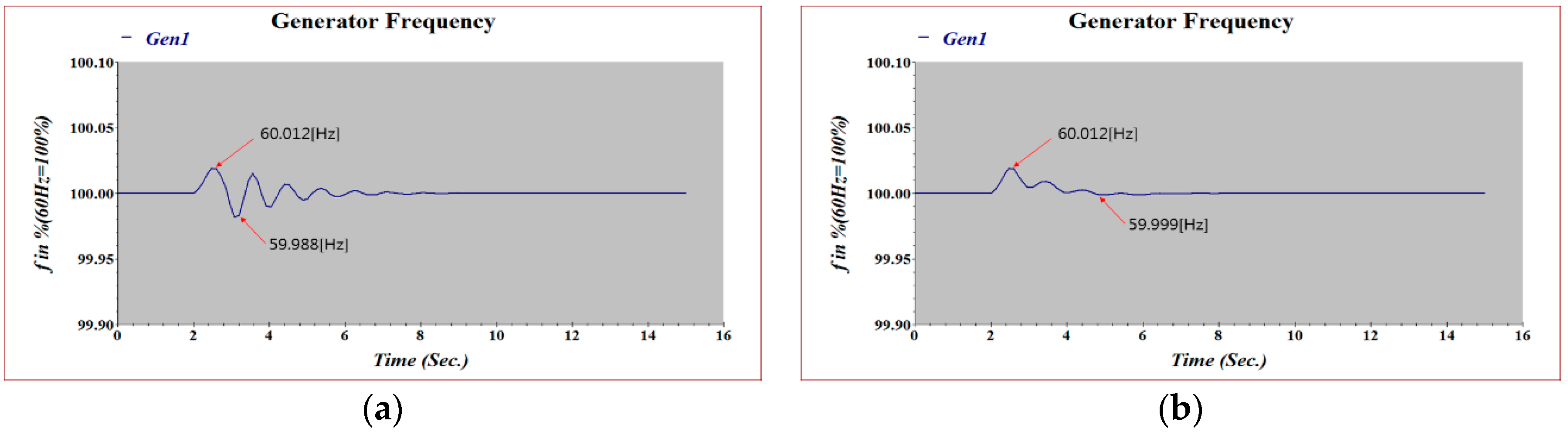
Figure 24.
Generator Frequency with/without OEL Function. (a) Without OEL at −10% Impact in Grid; (b) With OEL at −10% Impact in Grid.
Figure 24.
Generator Frequency with/without OEL Function. (a) Without OEL at −10% Impact in Grid; (b) With OEL at −10% Impact in Grid.
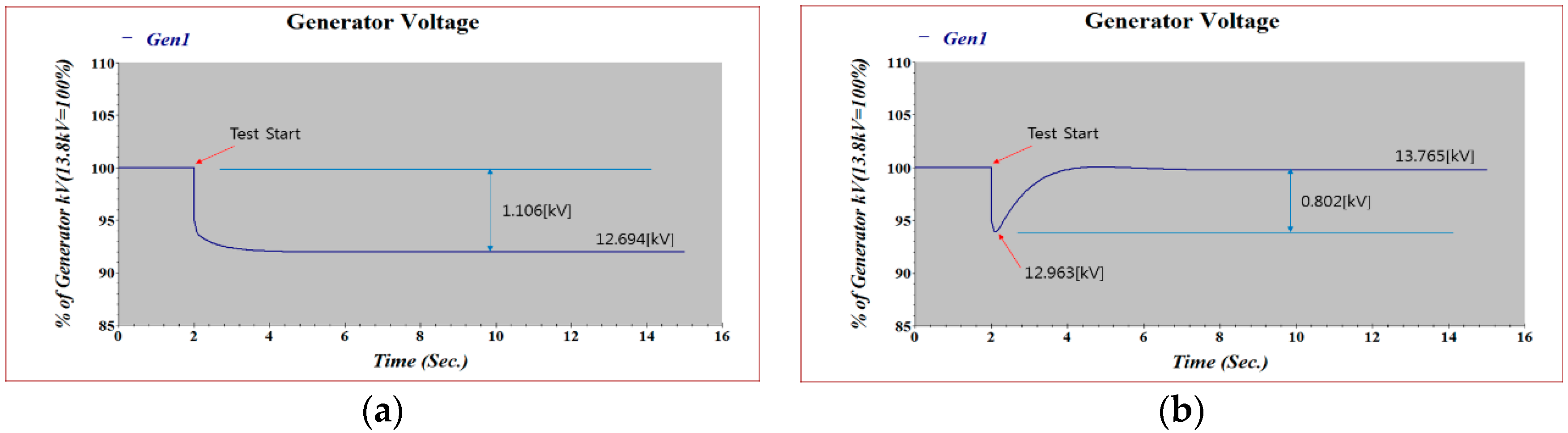
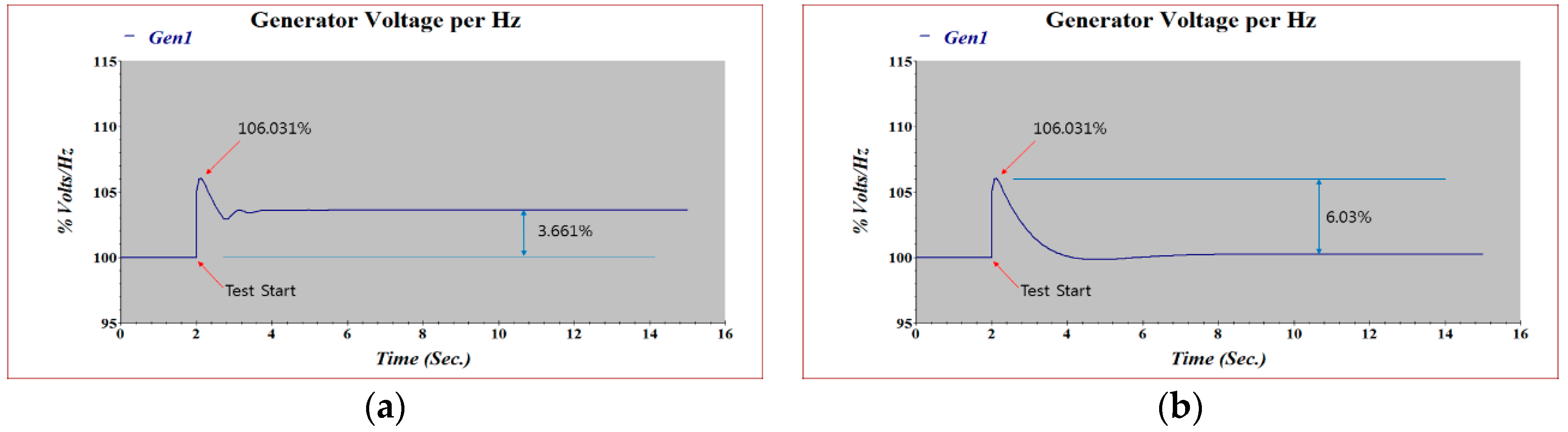
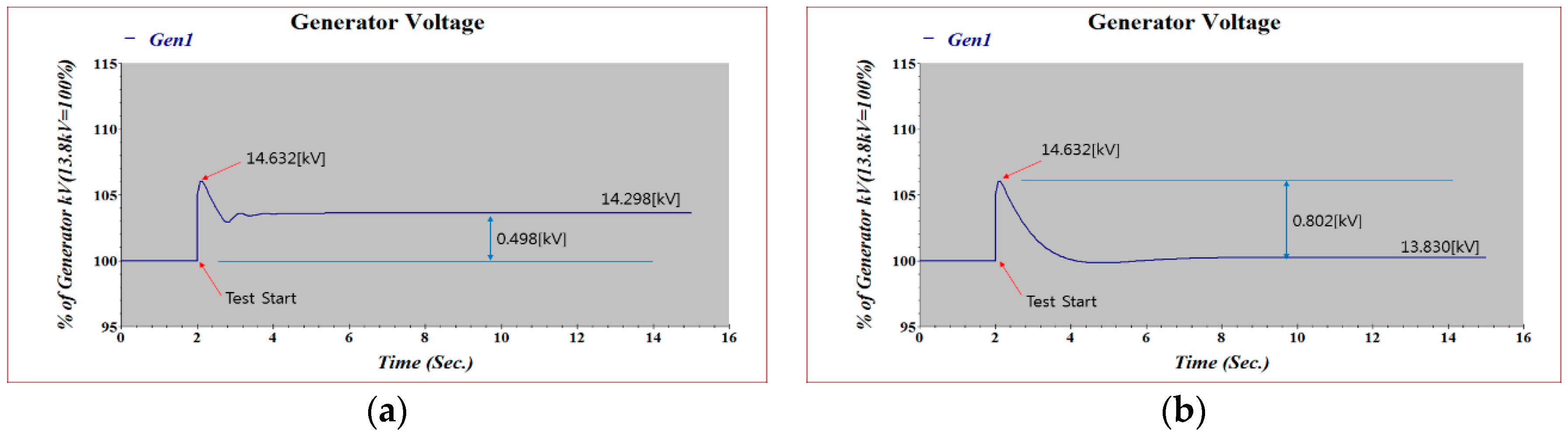
Figure 25.
Generator Voltage with/without OEL. (a) Without OEL at −10% Impact in Grid; (b) With OEL at −10% Impact in Grid.
Figure 25.
Generator Voltage with/without OEL. (a) Without OEL at −10% Impact in Grid; (b) With OEL at −10% Impact in Grid.
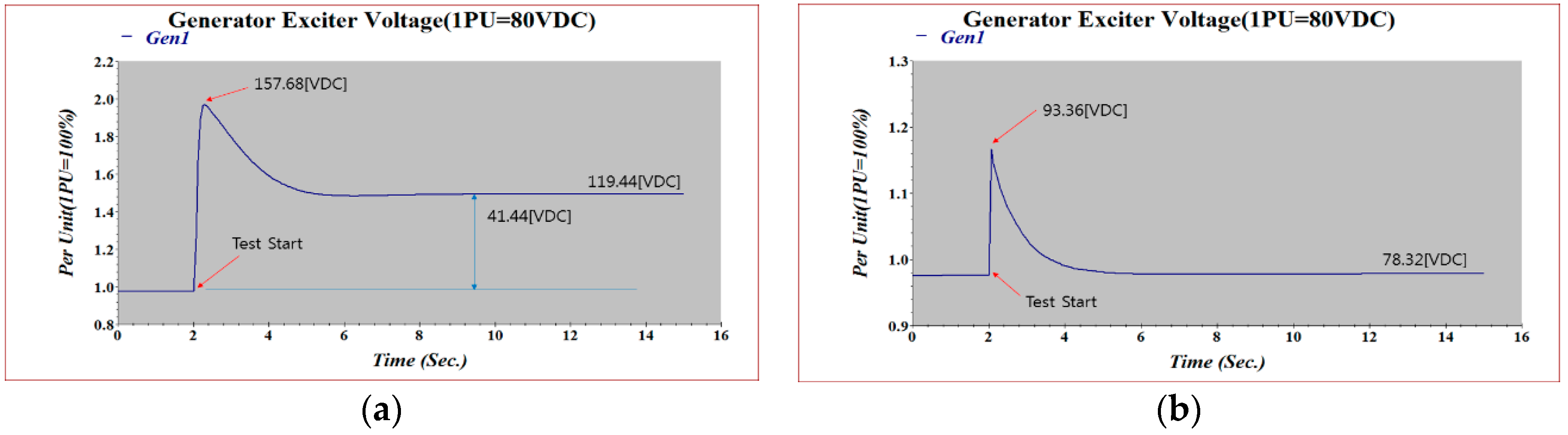
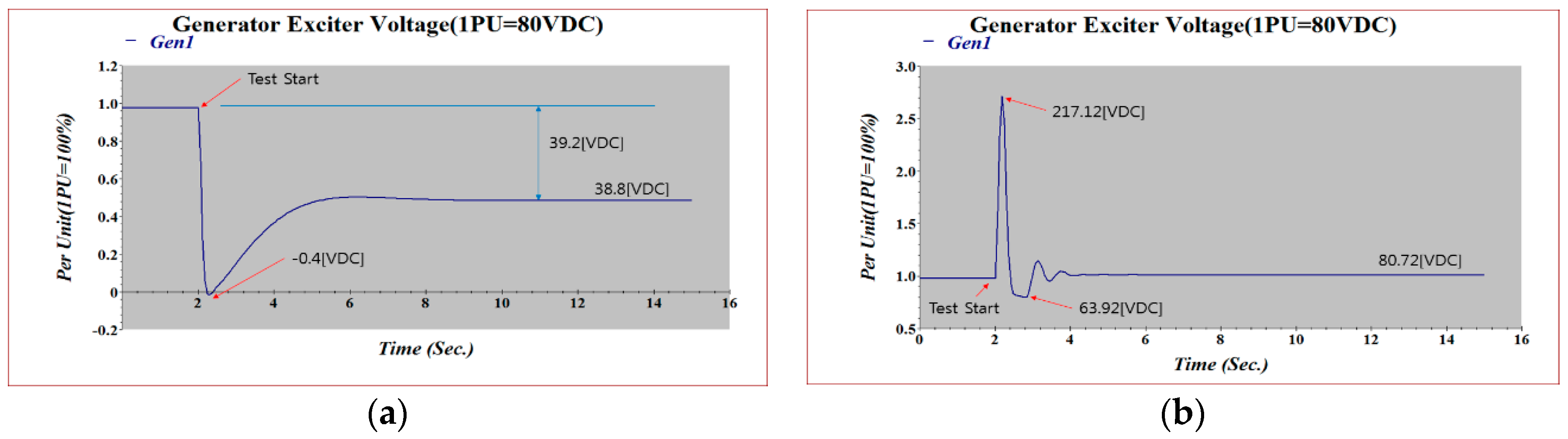
Figure 26.
Generator Field Voltage with/without OEL. (a) Without OEL at −10% Impact in Grid; (b) With OEL at −10% Impact in Grid.
Figure 26.
Generator Field Voltage with/without OEL. (a) Without OEL at −10% Impact in Grid; (b) With OEL at −10% Impact in Grid.
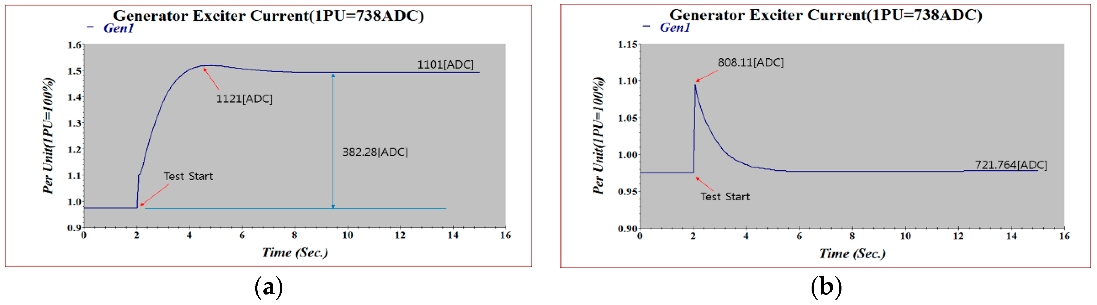
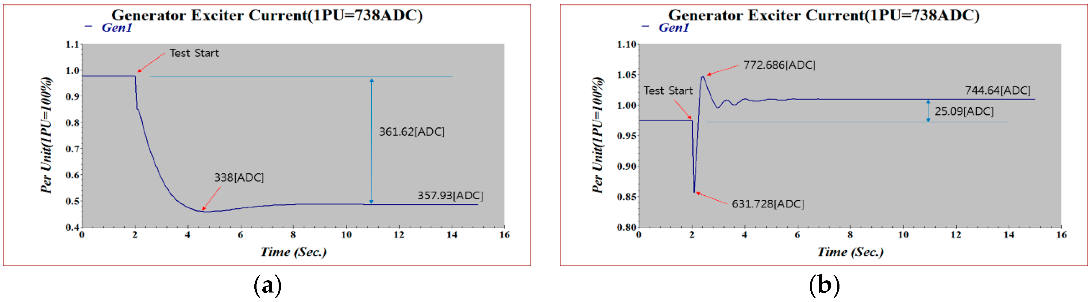
Figure 27.
Generator Field Current with/without OEL. (a) Without OEL at −10% Impact in Grid; (b) With OEL at −10% Impact in Grid.
Figure 27.
Generator Field Current with/without OEL. (a) Without OEL at −10% Impact in Grid; (b) With OEL at −10% Impact in Grid.
Figure 28.
Generator Power Phase Angles with/without Under Excitation Limiter (UEL). (a) Without UEL at −10% Impact in Grid; (b) With UEL at −10% Impact in Grid.
Figure 28.
Generator Power Phase Angles with/without Under Excitation Limiter (UEL). (a) Without UEL at −10% Impact in Grid; (b) With UEL at −10% Impact in Grid.
Figure 29.
Generator Reactive Power with/without UEL. (a) Without UEL at −10% Impact in Grid; (b) With UEL at −10% Impact in Grid.
Figure 29.
Generator Reactive Power with/without UEL. (a) Without UEL at −10% Impact in Grid; (b) With UEL at −10% Impact in Grid.
Figure 30.
Generator Active Power with/without UEL. (a) Without UEL at −10% Impact in Grid; (b) With UEL at −10% Impact in Grid.
Figure 30.
Generator Active Power with/without UEL. (a) Without UEL at −10% Impact in Grid; (b) With UEL at −10% Impact in Grid.
Figure 31.
Generator Speed with/without UEL. (a) Without UEL at −10% Impact in Grid; (b) With UEL at −10% Impact in Grid.
Figure 31.
Generator Speed with/without UEL. (a) Without UEL at −10% Impact in Grid; (b) With UEL at −10% Impact in Grid.
Figure 32.
Generator Current with/without UEL. (a) Without UEL at −10% Impact in Grid; (b) With UEL at −10% Impact in Grid.
Figure 32.
Generator Current with/without UEL. (a) Without UEL at −10% Impact in Grid; (b) With UEL at −10% Impact in Grid.
Figure 33.
Generator V/Hz with/without UEL. (a) Without UEL at −10% Impact in Grid; (b) With UEL at −10% Impact in Grid.
Figure 33.
Generator V/Hz with/without UEL. (a) Without UEL at −10% Impact in Grid; (b) With UEL at −10% Impact in Grid.
Figure 34.
Generator Frequency with/without UEL. (a) Without UEL at −10% Impact in Grid; (b) With UEL at −10% Impact in Grid.
Figure 34.
Generator Frequency with/without UEL. (a) Without UEL at −10% Impact in Grid; (b) With UEL at −10% Impact in Grid.
Figure 35.
Generator Voltage with/without UEL. (a) Without UEL at −10% Impact in Grid; (b) With UEL at −10% Impact in Grid.
Figure 35.
Generator Voltage with/without UEL. (a) Without UEL at −10% Impact in Grid; (b) With UEL at −10% Impact in Grid.
Figure 36.
Generator Field Voltage with/without UEL. (a) Without UEL at −10% Impact in Grid; (b) With UEL at −10% Impact in Grid.
Figure 36.
Generator Field Voltage with/without UEL. (a) Without UEL at −10% Impact in Grid; (b) With UEL at −10% Impact in Grid.
Figure 37.
Generator Field Current with/without UEL. (a) Without UEL at −10% Impact in Grid; (b) With UEL at −10% Impact in Grid.
Figure 37.
Generator Field Current with/without UEL. (a) Without UEL at −10% Impact in Grid; (b) With UEL at −10% Impact in Grid.
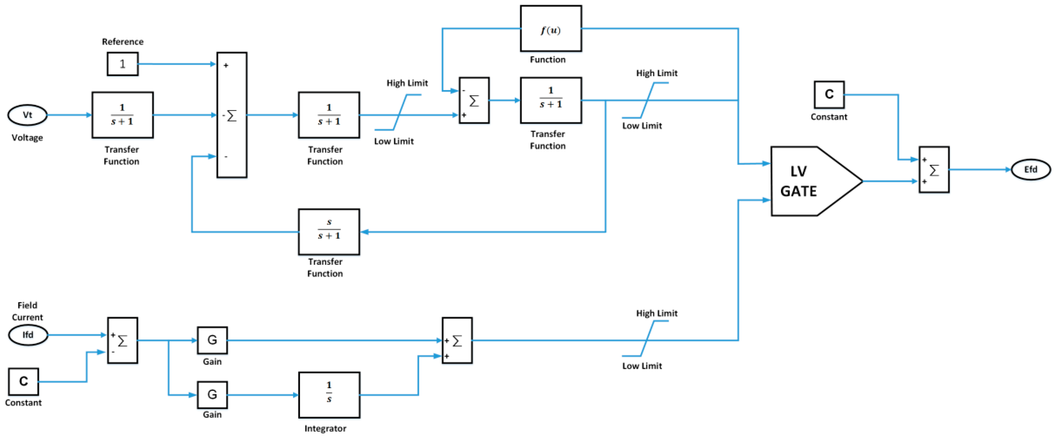
Figure 38.
Schematized Form of the OEL Model.
Figure 38.
Schematized Form of the OEL Model.
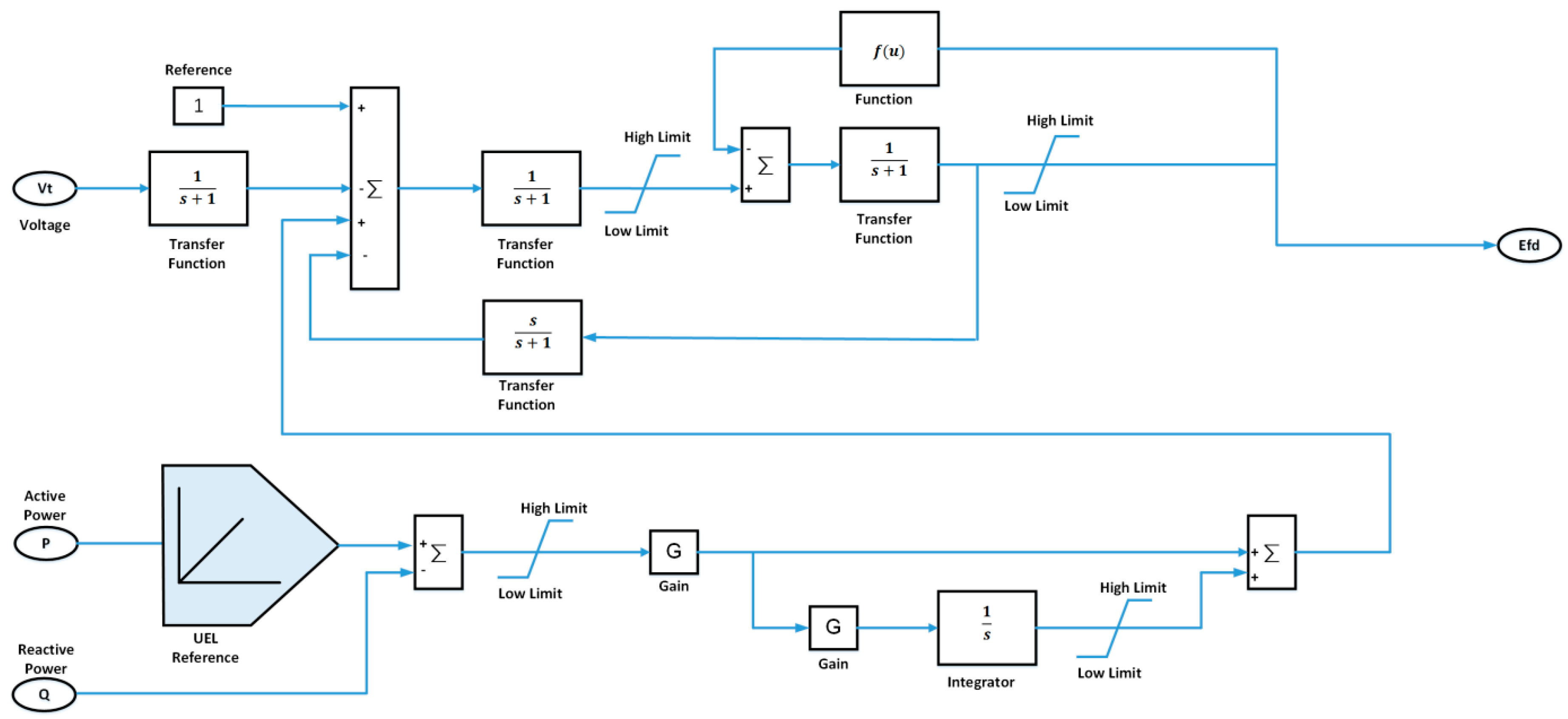
Figure 39.
Schematized Form of the UEL Model.
Figure 39.
Schematized Form of the UEL Model.
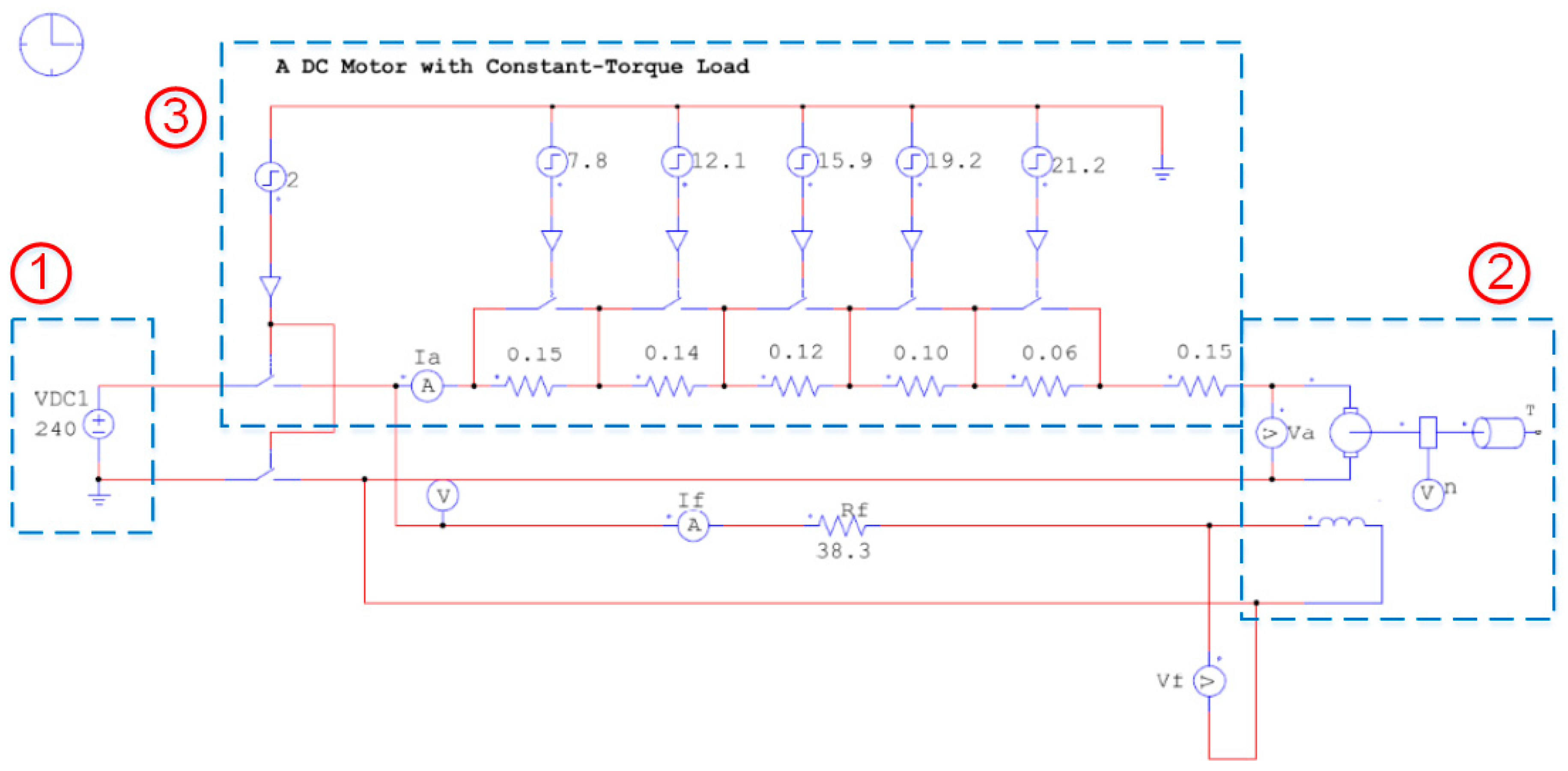
Figure 40.
PSIM (Powersim inc.) Simulation Circuit for the DC (Direct Current) Motor.
Figure 40.
PSIM (Powersim inc.) Simulation Circuit for the DC (Direct Current) Motor.
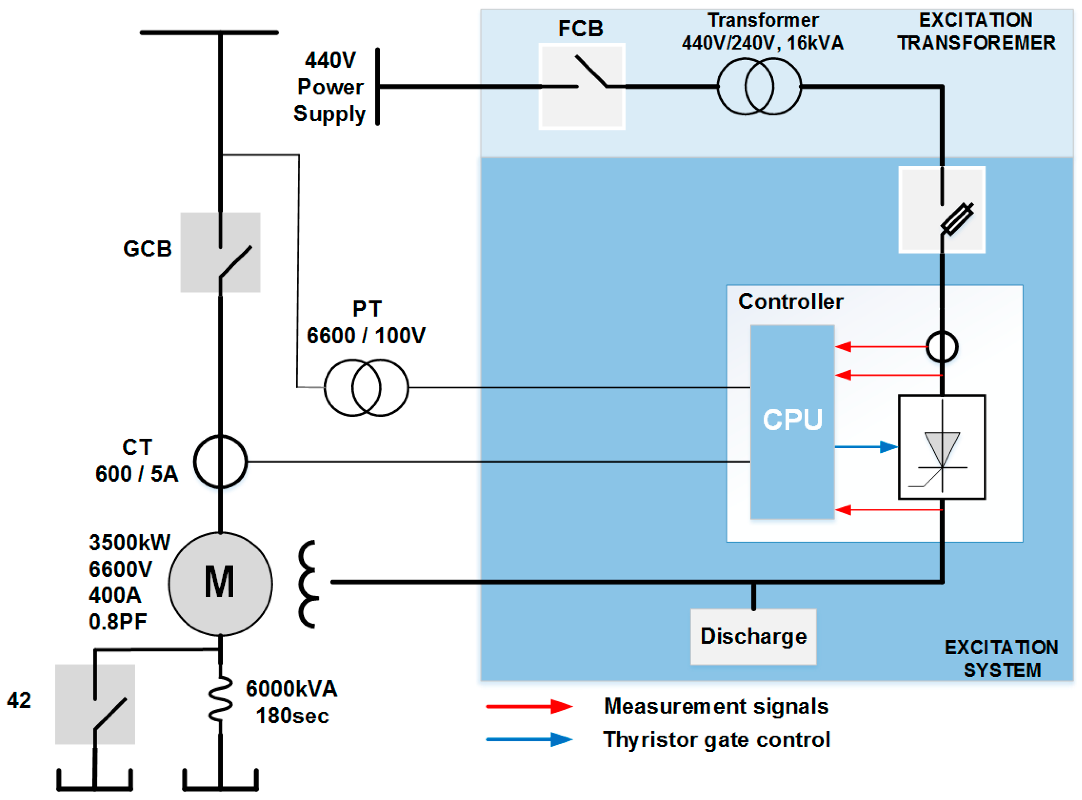
Figure 41.
Composition of the Excitation System of Synchronous Motor Architecture.
Figure 41.
Composition of the Excitation System of Synchronous Motor Architecture.
Figure 42.
Startup-checking Waveform of the Existing Excitation System.
Figure 42.
Startup-checking Waveform of the Existing Excitation System.
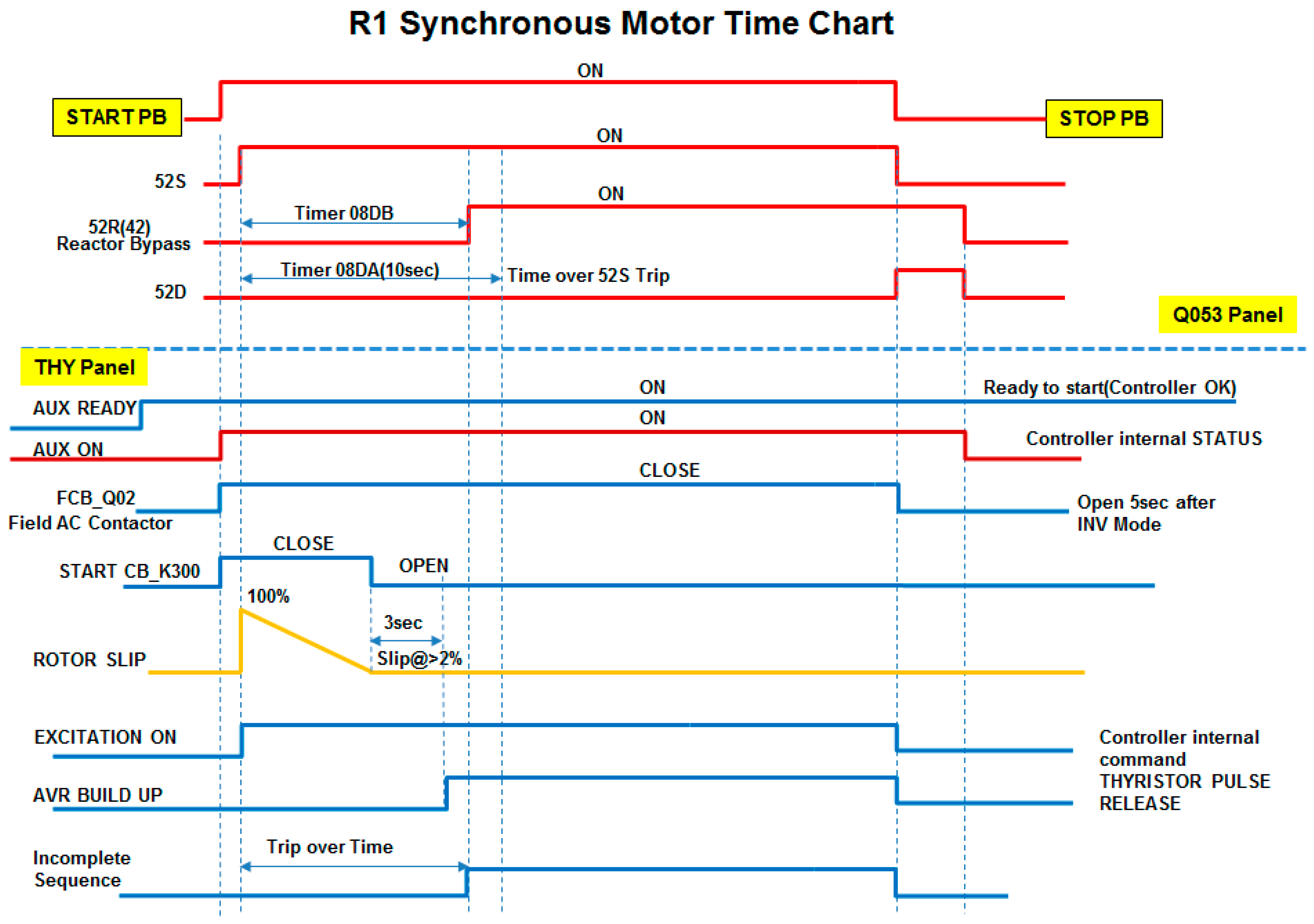
Figure 43.
Time Chart of the Proposed Excitation System.
Figure 43.
Time Chart of the Proposed Excitation System.
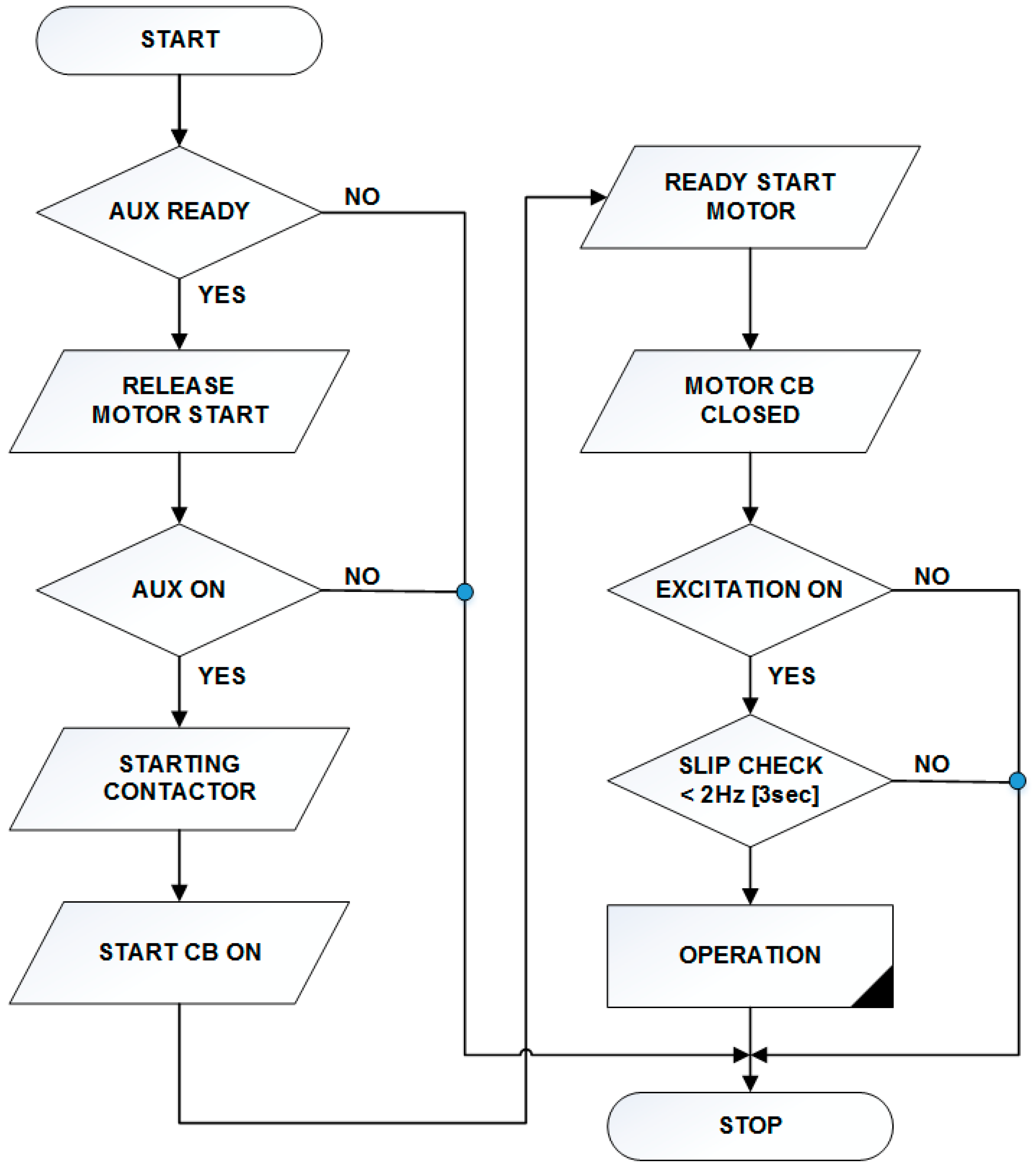
Figure 44.
Startup Sequence of the Synchronous Motor.
Figure 44.
Startup Sequence of the Synchronous Motor.
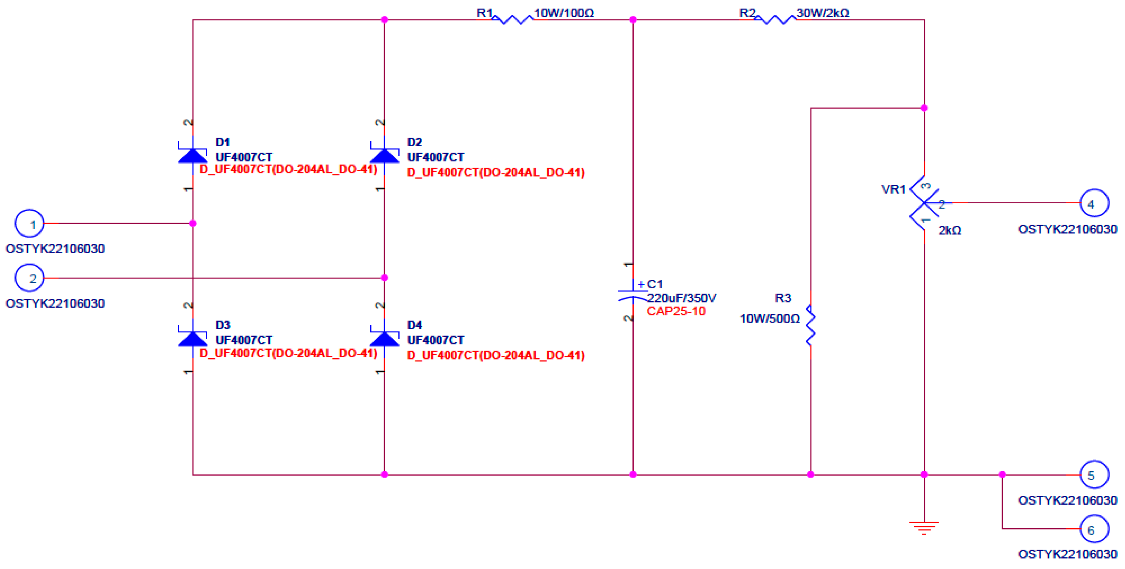
Figure 45.
Circuit for Slip Measuring.
Figure 45.
Circuit for Slip Measuring.
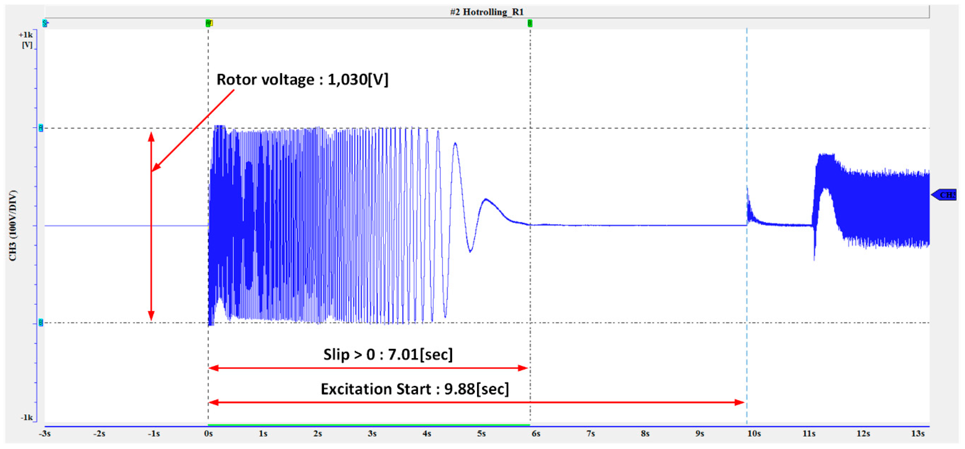
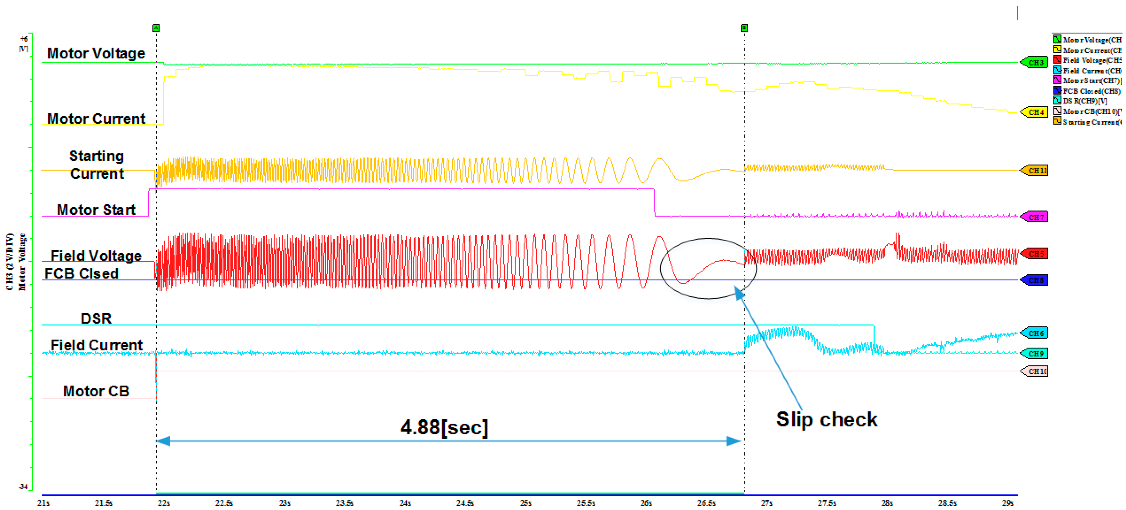
Figure 46.
Synchronous Motor Startup Waveform.
Figure 46.
Synchronous Motor Startup Waveform.
Table 1.
Specifications of the DC Motor.
Table 1.
Specifications of the DC Motor.
| kW | 37 | VOLT | 240 |
| ARM AMPS | 170 | FIELD | 1.87 |
| AMPS |
| FIELD | 240 | FIELD | 90 |
| VOLT | OHMS 25 °C |
| RPM | 1780 | TYPE | CDL409AT |
Table 2.
Specifications of the Synchronous Motor (Synchronous Motor).
Table 2.
Specifications of the Synchronous Motor (Synchronous Motor).
| Parameter | Value |
|---|
| Output | 3500 (kW) |
| Rated Voltage and Frequency | 6600 (V), 60 (Hz) |
| Field Voltage and Current | 220 (V), 305 (A) |
| Power Factor | 0.8 |
Table 3.
Over Voltage Trip Test.
Table 3.
Over Voltage Trip Test.
| Test | Input | Time/Result | Judgment |
|---|
| Over Voltage Trip Test | Measuring by impressing a generator voltage trip set value of 1.2 PU | Vt: 1.2 Pu, 60 Hz | Within 2 s/Confirmed | Pass |
Table 4.
V/Hz TRIP Test.
| Test | Input | Time/Result | Judgment |
|---|
| V/Hz TRIP Test | Measuring by changing the frequency at the rated generator voltage | Vt: 1.0 PU, 45 Hz | TRIP | Approx. 5 s/Confirmed | Pass |
Table 5.
OET Trip Test.
| Test | Input | Time/Result | Judgment |
|---|
| OET Trip Test | Measuring by adjusting the generator field current | IF: 0.4000 U | TRIP | Approx. 2 s/Confirmed | Pass |
Table 6.
Online OET Test.
Table 6.
Online OET Test.
| Test | Input | Time/Result | Judgment |
|---|
| Online OET Test | Measuring by adjusting the generator field current | IF: 2.0 PU | TRIP | Approx. 2 s/Confirmed | Pass |
Table 7.
Test Items at the Rated Generator Voltage/Current/Frequency.
Table 7.
Test Items at the Rated Generator Voltage/Current/Frequency.
| Test Items | Criteria | Result | Judgment |
|---|
| MASTER | BACKUP |
|---|
| KDR-1200D | KDR-1200D |
|---|
| P | Lead Phase 90° | 0.0000 | 0.0012 | 0.0002 | Pass |
| Lead Phase 45° | 0.7070 | 0.7080 | 0.7071 |
| In Phase | 1.0000 | 0.9998 | 1.0000 |
| Lag Phase 45° | 0.7070 | 0.7063 | 0.7069 |
| Lag Phase 90° | 0.0000 | 0.0000 | 0.0000 |
| Q | Lead Phase 90° | −1.0000 | −1.0000 | −1.0000 | Pass |
| Lead Phase 45° | −0.7070 | −0.7064 | −0.7069 |
| In Phase | 0.0000 | 0.0000 | 0.0000 |
| Lag Phase 45° | 0.7070 | 0.7081 | 0.7074 |
| Lag Phase 90° | 1.0000 | 1.0000 | 1.0000 |
Table 8.
PT Variant Generator Terminal Voltage.
Table 8.
PT Variant Generator Terminal Voltage.
| Test Items | Criteria | Result | Judgment |
|---|
| Master | Backup |
|---|
| Vrms | 16.6 V | 0.25 PU | 0.0000 | 0.0000 | Pass |
| 33.2 V | 0.50 PU | 0.4964 | 0.4966 |
| 66.39 V | 1.00 PU | 0.9999 | 1.0000 |
| 83 V | 1.25 PU | 1.2019 | 1.2018 |
| HZ | 48 Hz | 0.80 PU | 0.8003 | 0.8000 | Pass |
| 54 Hz | 0.90 PU | 0.9000 | 0.9001 |
| 60 Hz | 1.00 PU | 1.0001 | 1.0001 |
| 66 Hz | 1.10 PU | 1.1001 | 1.1000 |
Table 9.
VF, PCR1 and PCR2.
Table 9.
VF, PCR1 and PCR2.
| Test Items | Criteria | Result | Judgment |
|---|
| Master | Backup |
|---|
| VF | Take measurement by changing the field Voltage IF
(VF Rated = 82 V)
5.466 V/82 V | 0 V/0.0 V | 0.000 PU | 0.0001 | 0.0000 | Pass |
| 2.733 V | 0.500 PU | 0.4999 | 0.4999 |
| 5.466 V | 1.000 PU | 1.0000 | 1.0000 |
| 8.199 V | 1.500 PU | 1.5000 | 1.4999 |
Table 10.
IF, PCR1 and PCR2.
Table 10.
IF, PCR1 and PCR2.
| Test Items | Criteria | Result | Judgment |
|---|
| Master | Backup |
|---|
| IF | Take measurement by changing the field current IF
(IF Rated = 23 A)
[4.6 V/23 A] | 0 V | 0.00 PU | 0.0000 | 0.0000 | Pass |
| 2.3 V | 0.50 PU | 0.4985 | 0.4986 |
| 4.6 V | 1.00 PU | 0.9999 | 0.9998 |
| 6.9 V | 1.50 PU | 1.4970 | 1.4953 |
| 9.2 V | 2.00 PU | 1.9963 | 1.9944 |
| PCR1_IF | Take measurement by changing the PCR1 current
(IF Rated = 23 A)
[4.6 V/23 A] | 0 V | 0.00 PU | 0.0000 | 0.0000 | Pass |
| 2.3 V | 0.50 PU | 0.4987 | 0.4983 |
| 4.6 V | 1.00 PU | 1.0000 | 1.0000 |
| 6.9 V | 1.50 PU | 1.4980 | 1.4963 |
| 9.2 V | 2.00 PU | 1.9949 | 1.9950 |
| PCR2_IF | Take measurement by changing the PCR2 current
(IF Rated = 23 A)
[4.6 V/23 A] | 0 V | 0.00 PU | 0.0000 | 0.0000 | Pass |
| 2.3 V | 0.50 PU | 0.4965 | 0.4947 |
| 4.6 V | 1.00 PU | 1.0000 | 1.0001 |
| 6.9 V | 1.50 PU | 1.4915 | 1.4865 |
| 9.2 V | 2.00 PU | 1.9907 | 1.9814 |
Table 11.
ETF PT/CT Input Test.
Table 11.
ETF PT/CT Input Test.
| Classification | Ratio | ETP Input (Main) | ETP Input (Measure) | Remarks |
|---|
| Rated Generator Voltage | 13,800 V/115 V | A: 4.953 V; B: 4.764 V; C: 4.979 V | A: 4.626 V; B: 4.967 V; C: 5.038 V | - |
| Rated Generator Current | 4987 A/4.156 A | 4.081 V | - | - |
Table 12.
Test Items and Conditions.
Table 12.
Test Items and Conditions.
| Channel No. | Channel Name | Channel No. | Channel Name |
|---|
| AO-1 | Con_Signal1 | AO-5 | AO_VT |
| AO-2 | Con_Signal2 | AO-6 | AO_FREQ/AO_P(MW) |
| AO-3 | AO_IF | AO-7 | AO_Q(Mvar) |
| AO-4 | Balance_Meter | AO-8 | AO_Con_Signal |
Table 13.
Test Items Worked Flexibly (1).
Table 13.
Test Items Worked Flexibly (1).
| Test Items | Criteria | Master | Backup | Judgment |
|---|
| [Card1] | [Card1] |
|---|
| AO1 | Take measurement by changing the PCR firing control signals (0–10 V) | 0.0 PU | 0.00 V (±5%) | −0.011 | −0.024 | Pass |
| 0.5 PU | 2.50 V (±5%) | 2.461 | 2.448 |
| 1.0 PU | 5.00 V (±5%) | 4.939 | 4.927 |
| 1.5 PU | 7.50 V (±5%) | 7.42 | 7.41 |
| | | 2.0 PU | 10.00 V (±5%) | 9.89 | 9.88 | |
Table 14.
Test Items Worked Flexibly (2).
Table 14.
Test Items Worked Flexibly (2).
| Test Items | Criteria | Master | Backup | Judgment |
|---|
| [Card1] | [Card1] |
|---|
| AO2 | Take measurement by changing the PCR firing control signals (0–10 V) | 0.0 PU | 0.00 V (±5%) | −0.035 | −0.033 | Pass |
| 0.5 PU | 2.50 V (±5%) | 2.432 | 2.430 |
| 1.0 PU | 5.00 V (±5%) | 4.905 | 4.898 |
| 1.5 PU | 7.50 V (±5%) | 7.38 | 7.37 |
| 2.0 PU | 10.00 V (±5%) | 9.85 | 9.83 |


