Temporal Mixing Behavior of Conservative Solute Transport through 2D Self-Affine Fractures

Abstract

In this work, the influence of the Hurst exponent and Peclet number (Pe) on the temporal mixing behavior of a conservative solute in the self-affine fractures with variable-aperture fracture and constant-aperture distributions were investigated. The mixing was quantified by the scalar dissipation rate (SDR) in fractures. The investigation shows that the variable-aperture distribution leads to local fluctuation of the temporal evolution of the SDR, whereas the temporal evolution of the SDR in the constant-aperture fractures is smoothly decreasing as a power-law function of time. The Peclet number plays a dominant role in the temporal evolution of mixing in both variable-aperture and constant-aperture fractures. In the constant-aperture fracture, the influence of Hurst exponent on the temporal evolution of the SDR becomes negligible when the Peclet number is relatively small. The longitudinal SDR can be related to the global SDR in the constant-aperture fracture when the Peclet number is relatively small. As the Peclet number increases the longitudinal SDR overpredicts the global SDR. In the variable-aperture fractures, predicting the global SDR from the longitudinal SDR is inappropriate due to the non-monotonic increase of the longitudinal concentration second moment, which results in a physically meaningless SDR.

1. Introduction

It has been widely recognized that fractures can play an important role in the transport and fate of contaminants. Characterizing the spreading and mixing processes of conservative solute through the fractures is very important for the understanding of reaction rates and mass transport rates associated with nuclear waste disposal, enhanced oil recovery, and bioremediation [1,2,3,4,5,6]. Although, in recent decades, many studies have provided new insights into the mechanisms and properties of mixing processes in homogeneous and heterogeneous porous media [7,8,9,10,11,12,13,14,15,16,17], to date, little attention has been focused on mixing behavior in fractures.

Since the heterogeneity of geological formations is ubiquitous, a fundamental issue about the difference between spreading and mixing processes of conservative solute needs to be understood. Several authors [9,12,18] emphasized the difference between spreading and mixing. Spreading indicates the change of the spatial extent of a solute plume whereas mixing describes the process that uniformizes the concentration distribution of solute inside the plume. In other words, spreading leads to the stretching and deformation of a solute plume while mixing gives rise to dilution of a conservative solute with time. Thus, spreading and mixing are not the same, but complete conservative solute transport can be thought of as being composed of both spreading and mixing. For a conservative solute transport in a spatially variable velocity field, the spreading of the solute plume is driven by the differences in advection that deform and stretch out the plume along the streamlines, whereas at the same time molecular diffusion causes the mixing that smooths out the concentration gradients within the solute plume. There is a complex interaction between the spreading and mixing processes, especially in heterogeneous flow fields [19,20]. Due to the naturally-coupled property of spreading and mixing, separating the spreading and mixing process is challenging, but studying the temporal evolution of mixing is still useful and important for improving predictions of reactive transport and mixing. Describing conservative solute transport only by the spreading is valid for some applications (for example, risk analysis). However, due to the influence of the mixing behavior of reactants on rate of reaction, describing the transport with the mixing-controlled chemical reactions only by spreading is insufficient [3,21,22].

To this end, many efforts have been made to develop methods for quantifying mixing and spreading. Following Aris’s method of moments [23], the second central spatial moment of a conservative solute is a measure of spreading. This is because the spatial extent of the plume can be easily estimated based on the temporal evolution of spatial moments of the plume and is related to an apparent dispersion coefficient even for pre-asymptotic times [7,9,24,25]. In a homogeneous flow field, the second central spatial moment increases monotonically with time, which can be expected as a good measure for both spreading and mixing. This approach is invalid for a heterogeneous flow field where the second central spatial moment could decrease due to the convergence of streamlines [14,16,26]. Various metrics for quantifying mixing have been proposed.

Since the dilution caused by mixing is an irreversible process, Kitanidis [12] proposed the dilution index that measures the volume occupied by the solute plume. The dilution index is obtained from the statistical entropy (Shannon entropy) of the solute distribution. As opposed to the second central spatial moment, the dilution index is capable of quantifying true mixing and a mixing rate can be calculated by the rate of change of the entropy. The dilution index is useful not only for conservative solute transport but also for reactive transport [27]. The ratio of actual to theoretical maximum dilution index can be an indicator of the influence of incomplete mixing on reactive transport [15,28]. Moreover, based on the original concept of the dilution index, the flux-related dilution index that describes dilution as “act of distributing a given solute mass flux over a larger water flux” was proposed by Rolle et al. [14] for steady-state transport with continuous injection mode.

From the view of stochastic hydrogeology, the concentration distribution of a solute plume can be decomposed into a cross-sectional mean and a fluctuation about that mean. The concentration variance method has been proposed as a measure of mixing [11,29,30]. In addition to the dilution index and concentration variance, the mixing can be alternatively quantified by the scalar dissipation rate (SDR) which is determined from the time derivative of the integral of squared concentration within the solute plume [22,31]. Although the SDR was proposed for the study of turbulent flow and combustion, several studies [32] have shown that the SDR can be also applied to a variety of problems of subsurface contaminant transport (e.g., compound-specific transport, conservative solute transport, and multicomponent reactive transport). Le Borgne et al. [31] investigated the temporal evolution of the SDR in heterogeneous porous media and demonstrated the occurrence of a non-Fickian scaling of mixing. Bolster et al. [7] used the SDR to decompose the global mixing state into a dispersive mixing state and a local mixing state. Jha et al. [33] applied the SDR to quantify the mixing in a viscously unstable flow. Dreuzy et al. [21] considered that mixing resulted from competition between velocity fluctuations and local scale diffusion, and they proposed a new decomposition of mixing into potential mixing and departure rate. This new decomposition of mixing showed a generic characterization and could offer new ways to establish a transport equation with consideration of both advection, spreading, and mixing. A comparison of different transport models can be found in [10]. A series of analytical solutions for the SDR was derived in non-conservative transport systems by Engdahl, Ginn, and Fogg [32]. Furthermore, previous studies [7,21,31] in porous media showed that the transverse mixing generating the concentration gradients in the transverse direction influenced longitudinal mixing. If the global mixing was dominated by the spreading at asymptotical time, the transverse mixing could be negligible and the global mixing could be predicted by the longitudinal mixing. However, these current studies on the SDR are limited to specific homogeneous or heterogeneous porous media. Since anomalous (non-Fickian) transport has been observed in single rough fractures [34,35,36,37,38] and mixing and spreading could play an important role in fractures, the study of the performance, characteristic, and evolution of the SDR in other important subsurface geological formations (e.g., single rough fractures) needs further investigation.

The primary objective of this work is to investigate the effects of the Hurst exponent (which can indicate the roughness features of the fracture walls) and Peclet number on the temporal behavior of mixing. The validity of using longitudinal mixing to predict global mixing was evaluated in self-affine fractures. Two groups of different self-affine fractures were considered and denoted as the constant-aperture fracture and the variable-aperture fracture. The computational fluid dynamics (CFD) simulations of the flow field and solute transport in fractures were implemented. There are three major contributions here relative to previous work. The first is to show the capability of the SDR for characterizing the mixing in self-affine fractures. The second is to quantify the influence of the Hurst exponent and the Peclet number on the SDR scaling in constant-aperture fractures and the variable-aperture fractures. The third is to test and evaluate the validity of using the longitudinal mixing to predict the global mixing in self-affine fractures.

2. Methodology

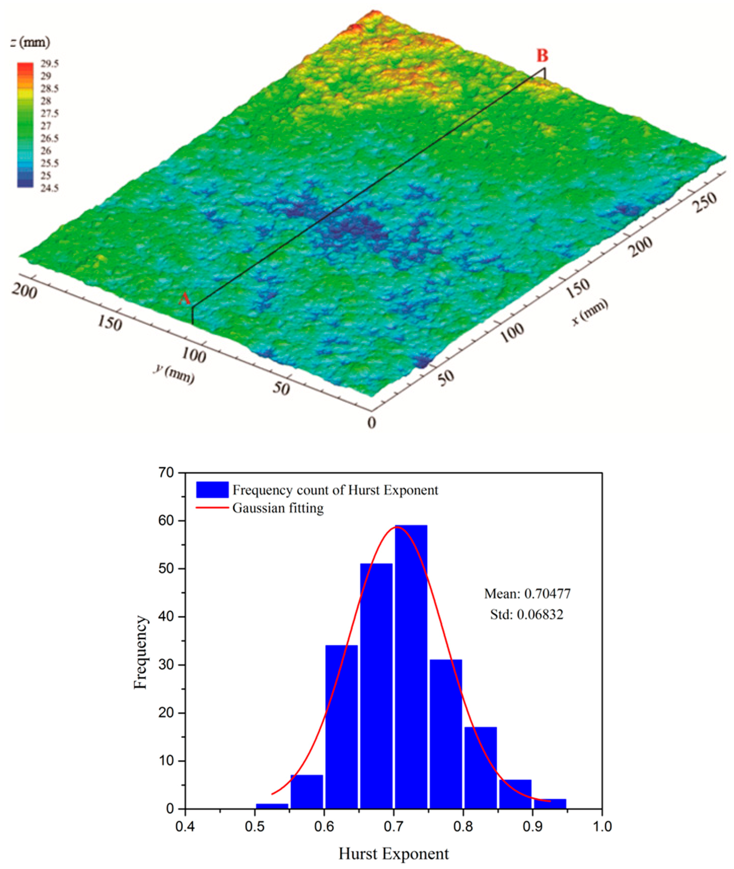
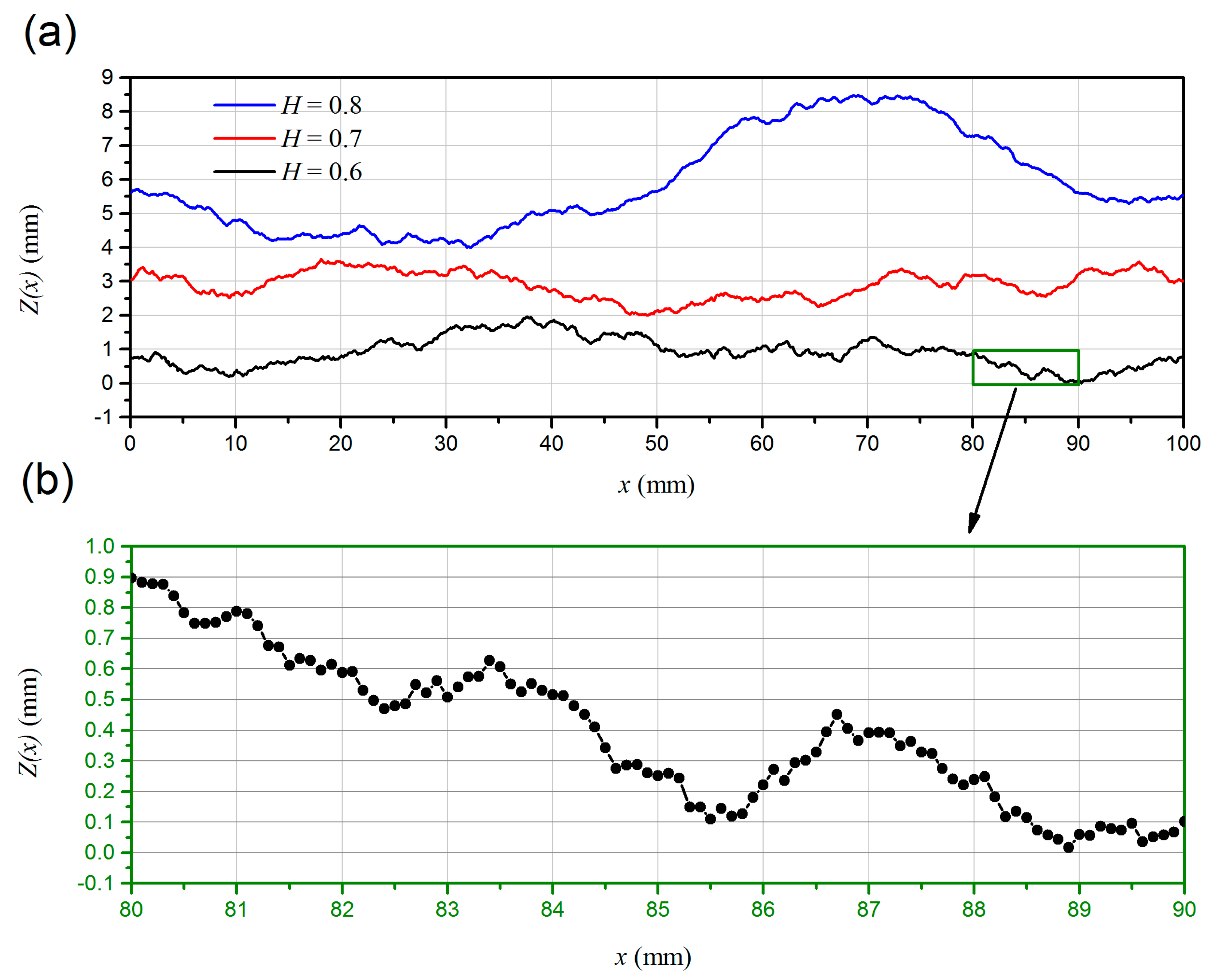
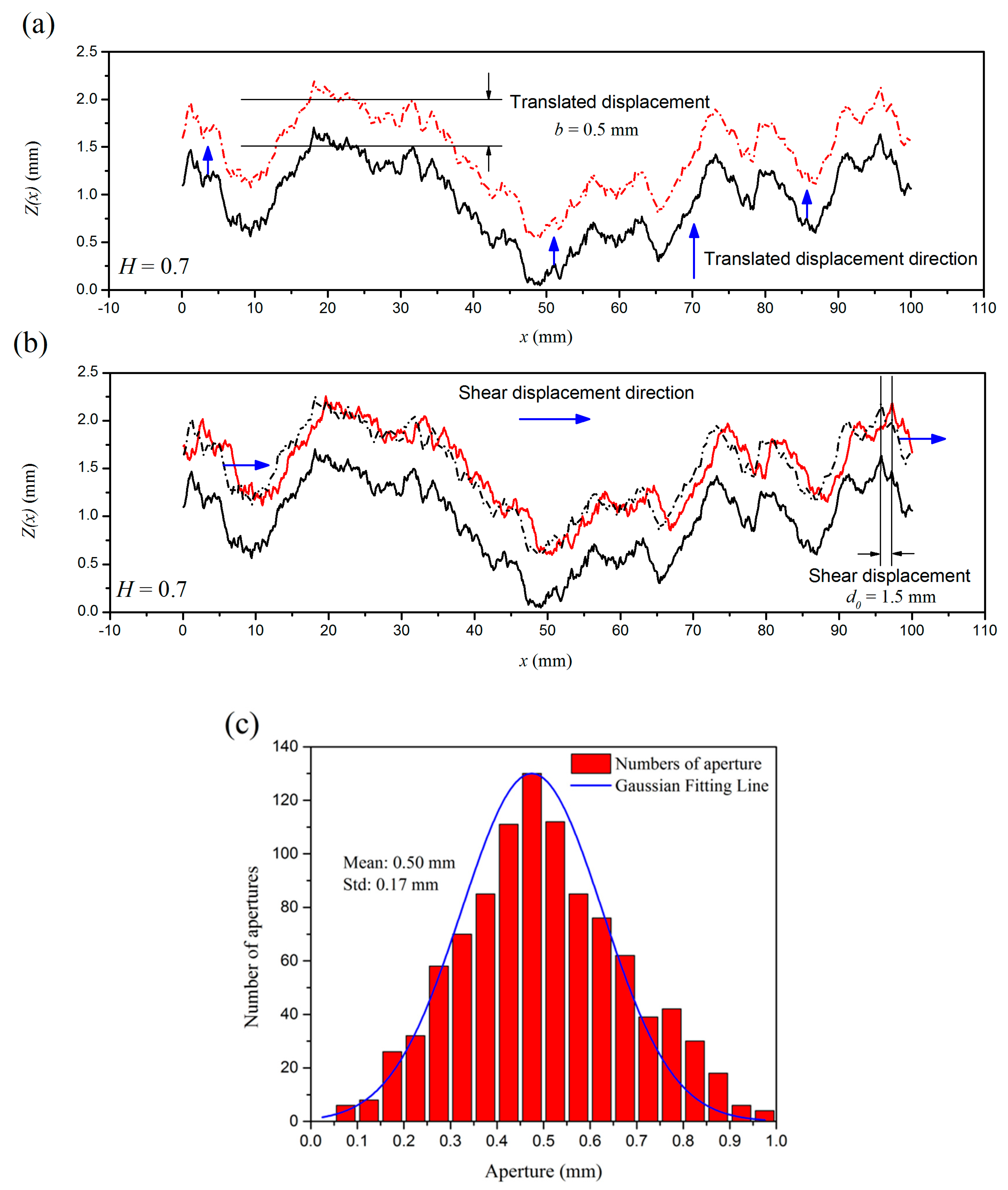
2.1. Fracture Generation

Previous studies [39] on the morphology of natural fracture walls indicated that the walls of natural fractures could be characterized as statistical self-affine distributions. The mathematical characterization of the self-affine rough fracture wall was briefly reviewed here. A two-dimensional single fracture was considered, whose height is defined by a single-value function $Z\left(x\right)$ and the statistical self-affine property of the height can be expressed as:

$${\lambda }^{H}Z\left(x\right)=Z\left(\lambda x\right)$$

(1)

where $H$ indicates the magnitude of the roughness or the so-called Hurst exponent varying from 0 to 1 and $\lambda$ is a scaling factor. $Z\left(x\right)$ can be thought of as a function of an independent spatial or temporal variable $x$. For a self-affine fracture wall, the stationary increment [$Z\left(x+h_x\right)-Z\left(x\right)$] over the distance $h_x$ follows a Gaussian distribution with mean zero. Thus, for the arbitrary$\lambda$, the mean and variance of the increments can be expressed as:

$$\langle Z\left(x+\lambda h_x\right)-Z\left(x\right)\rangle =0$$

(2)

$${\sigma }^2\left(\lambda \right)={\lambda }^{2H}{\sigma }^2\left(1\right)$$

(3)

where $\langle ·\rangle$ represents the mathematical expectation. For the different distances, the variance ${\sigma }^2\left(\lambda \right)$ is defined as a function of $\lambda$:

$${\sigma }^2\left(\lambda \right)=\langle {\left[Z\left(x+\lambda \right)-Z\left(x\right)\right]}^2\rangle$$

(4)

$${\sigma }^2\left(\lambda h_x\right)=\langle {\left[Z\left(x+\lambda h_x\right)-Z\left(x\right)\right]}^2\rangle$$

(5)

Then, depending on Equation (3):

$${\sigma }_{\lambda h_x}^2={\lambda }^{2H}{\sigma }_{h_x}^2$$

(6)

$${\sigma }_{\lambda h_x}={\lambda }^H{\sigma }_{h_x}$$

(7)

where ${\sigma }_{\lambda h_x}^2$ and ${\sigma }_{h_x}^2$ represent the variances of increments with different distances $\lambda h_x$ and $\lambda$, respectively.

Based on the self-affine scaling law given by Equations (1)–(7), a number of algorithms (e.g., the successive random additions, the randomization of the Weierstrass-Mandelbrot function, and the Fourier transformation) have been developed for synthetic self-affine fracture generation. In the present study, the successive random addition algorithm [40] was used to generate the synthetic self-affine fracture wall. It should be noted that to generate the self-affine fracture wall, the desired Hurst exponent must be selected. For this, the rough surface morphology of the bottom fracture wall of a single-fracture dolomite rock block (of 280 × 210 × 70 mm in size) was measured by using a 3D stereo-topometric measurement system (ATOS II from GOM mbH, Braunschweig, Germany). Preparation of this single-fracture dolomite rock block has been described in [41]. A 3D model of the fracture wall surface was generated by ATOS II using non-contact optical scanning technique [42]. A raw dataset of fracture surface heights from the dolomite rock fracture sample was obtained with a spatial resolution of ~250 µm (See Figure 1). From variogram analysis [43], the self-affinity of dolomite rock surface was evaluated. The distribution of Hurst exponent values was examined over 200 profiles along the longitudinal direction (for example, A-B profile in Figure 1). The calculated Hurst exponent values were between 0.55 and 0.91, where Hurst exponent between 0.6 and 0.8 covers ~90% of profiles. Thus, due to the computational cost, three different Hurst exponents were selected (i.e., H = 0.6, H = 0.7, and H = 0.8).

Once the desired Hurst exponent was selected, the self-affine fracture wall was generated by the successive random addition algorithm. Figure 2 shows the generated self-affine fracture walls with H = 0.8, H = 0.7, and H = 0.6, respectively. It can be seen from Figure 2 that the larger Hurst exponent leads to a higher spatial correlation and a smoother wall.

In self-affine fractures, the aperture distribution can have a significant influence on the spreading and mixing processes. The reconstruction of the aperture field from a pair of generated fracture walls is dependent upon the way in which the walls are oriented relative to each other. Note that the Hurst exponent could be different for the top and bottom fracture walls. However, our aim here is not to perform an exhaustive investigation for all possibilities. It is assumed that the reconstructed fracture is two-dimensional, uniform mineral component, there is no contact area (no zero-aperture region), and the Hurst exponent for both of the top and bottom fracture walls is the same. Two possibilities to reconstruct the rough fracture aperture field from the specific self-affine fracture walls were considered. First, a constant-aperture rough fracture was introduced, where the top fracture wall was a replica of the bottom fracture wall translated a distance $\overline{b}$ normal to the mean plane (See Figure 3a). In this case, the fracture walls are rough and self-affine, but the local aperture $b\left(x\right)$ is constant and equal to$\overline{b}$. Alternatively, the variable-aperture rough fracture was studied, where the top fracture wall was a replica of the bottom wall. The bottom wall was sheared along the horizontal direction by a displacement $d_0$ and then translated a distance $\overline{b}$ normal to the mean plane (See Figure 3b). Obviously, the two walls of the reconstructed fracture with shear displacement $d_0$do not overlap and the local aperture is a function of the horizontal location x. Based on the self-affine scaling law, Wang, et al. [44] developed the shear displacement model to obtain the aperture field with Gaussian distribution. The local aperture $b\left(x\right)$ is given by:

$$S_2\left(x\right)=S_1\left(x+d_0\right)+\overline{b}$$

(8)

$$b\left(x\right)=\{\begin{array}{c}{S}_2\left(x\right)-S_1\left(x\right)\\ 0\end{array} \begin{array}{c}\mathrm{if} S_2\left(x\right)>S_1\left(x\right)\\ \mathrm{otherwise}\end{array}$$

(9)

where $S_1\left(x\right)$ and $S_2\left(x\right)$ are the top and bottom fracture walls, respectively. Figure 3c shows that when the Hurst exponent of the self-affine fracture wall is H = 0.7, the aperture field of the variable-aperture rough fracture follows a Gaussian distribution with the mean aperture $\overline{b}=0.5$ mm and the standard deviation of the aperture ${\sigma }_b=0.17$ mm.

In this study, the total length of the generated self-affine fracture wall is set as 100 mm and the horizontal distances between two adjacent points in the self-affine fracture wall were equal to 0.1 mm (see Figure 2b). Three self-affine fracture walls with H = 0.6, H = 0.7, and H = 0.8 were generated by the successive random addition algorithm. Each self-affine fracture wall was used to reconstruct the constant-aperture fracture and the variable-aperture fracture, respectively. Thus, there were six fractures in this study. The coefficient of variation (COV) was set to 0.35 for the variable-aperture fracture.

2.2. Computational Fluid Dynamics (CFD) Simulations of the Flow Field and Solute Transport in Single Rough Fractures

Since the mixing behavior is highly dependent on the flow field [8,9,16,45], the flow field in a single rough fracture was solved directly by using the Navier-Stokes and continuity equations for isothermal, incompressible, and homogenous single Newtonian steady flow:

$$\nabla ·\mathit{u}=0$$

(10)

$$\rho \left(\mathit{u}·\nabla \mathit{u}\right)-\nabla \left(\mu \nabla \mathit{u}\right)=-\nabla p$$

(11)

where $\rho$ is the density of fluid, $\mathit{u}=\left[u,w\right]$ is the velocity vector, $p$ is the fluid pressure, and $\mu$ is the dynamic viscosity of fluid. Two given pressure values were implemented at the inlet and outlet boundary. The steady-state flow field was solved by the pressure drop over the entire fracture.

Transient solute transport in a single self-affine fracture was described by the advection-diffusion equation for conservative non-sorbing solute transport:

$$\frac{\partial c}{\partial t}=-\nabla ·\left(\mathit{u}c\right)+D_m{\nabla }^{2}c$$

(12)

where $c$ is the solute concentration, $t$ is time, and $D_m$ is the molecular diffusion coefficient. The velocity vector in Equation (12) is from the flow field based on solution of Equations (10) and (11). It is assumed that the initial concentrations were given by:

$$c_{}\left(x, t=0\right)=\{\begin{array}{c}\frac{m_0}{b\left(x\right)\ast \Delta L\ast W} \mathrm{if} x_L^{*}<x<x_L^{*}+\Delta L\\ 0 \mathrm{otherwise}\end{array}$$

(13)

where $m_0$ is the mass of injected solute, $b\left(x\right)$ is the local aperture, W is the width of fracture in the out of plane direction (equal to 1 m in the 2D problem) and $\Delta L$ is the width of injected solute. The $\Delta L$ is constant for all of simulations and assumed as $\Delta L/L=0.001$, where the L is the length of the whole fracture. To avoid boundary effects, the initial injection location of the solute e mass is shifted downstream from the fracture inlet by a distance of $x_L^{*}=0.01L$. The inlet and outlet boundary conditions for transient solute transport were specified as:

$$c\left(0,t\right)=0t\ge 0$$

(14)

$$\partial c\left(L,t\right)/\partial n=0t\ge 0$$

(15)

where n represents the normal direction to the outlet boundary.

2.3. Mixing: Scalar Dissipation Rate (SDR)

Mixing can be described by the SDR that is a global mixing measure based on the integral of concentration gradients. Recently, several studies have focused on the SDR evolution and scaling properties during solute transport in porous media [7,10,13,21,27,31,32,46]. However, all of those studies on SDR were restricted to porous media. The study on the SDR evolution in rough fractures is still limited, which motivates our investigation. The SDR of a conservative scalar is given by:

$$\chi \left(t\right)={{\displaystyle \int }}_{\mathsf{\Omega }}^{}{D}_m\nabla c\left(x,t\right)·\nabla c\left(x,t\right)dx$$

(16)

To obtain the SDR by using the Equation (16), the local concentration gradients needs to be determined. However, due to the occurrence of the sharp concentration gradient over small distances in the relatively heterogeneous flow field, a very fine numerical discretization for both of the flow and the concentration field is required to obtain an accurate quantification of concentration gradients, which results in the huge computational cost. Le Borgne et al. [31] showed that the SDR can be approximated from the concentration second moment (the integral of the squared concentrations). After multiplying Equation (12) by $c\left(x,t\right)$ and integrating over the entire domain:

$$\begin{array}{c}\frac{1}{2}\frac{\partial }{\partial t}{{\displaystyle \int }}_{\mathsf{\Omega }}^{}c{\left(x,t\right)}^{2}d\mathsf{\Omega }+\frac{1}{2}{{\displaystyle \int }}_{\mathsf{\Omega }}^{}\nabla ·\left[\mathit{u}c{\left(x,t\right)}^2\right]d\mathsf{\Omega }=\frac{1}{2}{D}_m{{\displaystyle \int }}_{\mathsf{\Omega }}^{}\nabla ·\nabla c{\left(x,t\right)}^{2}d\mathsf{\Omega }\\ -{{\displaystyle \int }}_{\mathsf{\Omega }}^{}{D}_m\nabla c\left(x,t\right)·\nabla c\left(x,t\right)d\mathsf{\Omega }\end{array}$$

(17)

Assuming that the fractured domain is infinite, there is no mass flux out of the domain, and the flow field is divergence-free, the terms involving a divergence operator in Equation (17) are zero. Then it can obtain:

$$\chi \left(t\right)=-\frac{1}{2}\frac{d{M}^2\left(t\right)}{dt}=D_m{{\displaystyle \int }}_{\mathsf{\Omega }}^{}\nabla ·\nabla c{\left(x,t\right)}^{2}d\mathsf{\Omega }$$

(18)

where $M^2\left(t\right)$ is the concentration second moment and can be expressed as:

$$M^2\left(t\right)={{\displaystyle \int }}_{\mathsf{\Omega }}^{}c{\left(x,t\right)}^{2}d\mathsf{\Omega }$$

(19)

Le Borgne et al. (2010) reported that the results from using Equation (18) instead of Equation (16) are more accurate than from using Equation (16) directly and the calculation for Equation (18) is computationally more efficient. In this study, the temporal mixing state is obtained from Equation (18).

For an infinite 1D homogeneous domain with zero velocity Fick’s Law of diffusion can be used to describe the spatial distribution of solute concentration. The corresponding analytical solution for the concentration distribution in the absence of reaction is given by:

$$c_0\left(x,t\right)=\frac{m_0}{\sqrt{4\pi D_{m}t}}\exp (-\frac{x^2}{4\pi D_m})$$

(20)

By integrating the square of Equation (20) over all domains, the corresponding concentration second moment can be expressed as:

$${{\displaystyle \int }}_{\mathsf{\Omega }}^{}{c}_0{\left(x,t\right)}^{2}d\mathsf{\Omega }=\frac{m_0^2}{\sqrt{8\pi D_{m}t}}=M_0^{}\left(t\right)$$

(21)

From Equation (18), the analytical 1D SDR solution can thus be expressed as:

$${\chi }_0\left(t\right)=-\frac{1}{2}\frac{d{M}_0^{}\left(t\right)}{dt}=\frac{1}{8}\frac{m_0^2}{\sqrt{2\pi D_m}}{t}^{-\frac{3}{2}}$$

(22)

3. Results and Discussion

3.1. Model Setup

In this study, the water with standard properties at 20 °C (e.g., $\rho$ = 998.2 kg/m³ and $\mu$ = 1.002 × 10⁻³ Pa∙s) was used to saturate the void space in the fractures. The typical conservative solute transport (e.g., ${\mathrm{Cl}}^{-}$ in water) and the corresponding $D_m=2.03\times {10}^{-9}{\mathrm{m}}^2/\mathrm{s}$ were assumed depending on the reference of [47]. The matrix of the fracture was assumed impermeable and the rough fracture walls were considered as non-slip boundaries. As background flow, the steady-state flow was induced by a given pressure drop over the entire fracture. The solved flow field serves as the input for the transient solute transport model. The flow field and transient solute transport models based on Equations (10)–(16) were implemented in the COMSOL Multiphysics package version 5.2 (COMSOL Inc., Burlington, MA, USA) using the Galerkin finite-element method [48]. In order to ensure numerical stability and accuracy, the fracture domain was discretized into ~152,000 triangular elements. The number of triangular elements was determined by the mesh independence analysis. Under the same pressure gradient ($-\nabla p=185 \mathrm{Pa}/\mathrm{m}$), the steady-state flow rate changes about 0.95% (from 9.550 $\times {10}^{-4}{\mathrm{m}}^3/\mathrm{s}$ to 9.641 $\times {10}^{-4}{\mathrm{m}}^3/\mathrm{s}$) as the number of triangular elements increases by about 104% (from 152,000 to 310,000). This indicates that 152,000 triangular elements are sufficient to provide stable and accurate numerical results.

The Peclet number, $Pe={\tau }_D/{\tau }_a=\overline{u}\overline{b}/D_m$, was defined by the ratio of the characteristic diffusion time (${\tau }_D={\overline{b}}^2/D_m$) to the characteristic advection time (${\tau }_a=\overline{b}/\overline{u}$) where the $\overline{u}$ is the mean flow velocity in the fractures. In each simulation, three different Pe values (Pe = 10, Pe = 100, and Pe = 1000) were considered. Without loss of generality, Figure 4 shows the flow fields in variable-aperture and constant-aperture fractures for a self-affine fracture wall with H = 0.6 and Pe = 1000. Figure 5 shows the results for both constant-aperture and variable-aperture fractures when the Pe is set as 1000 and Hurst exponent is equal to 0.6.

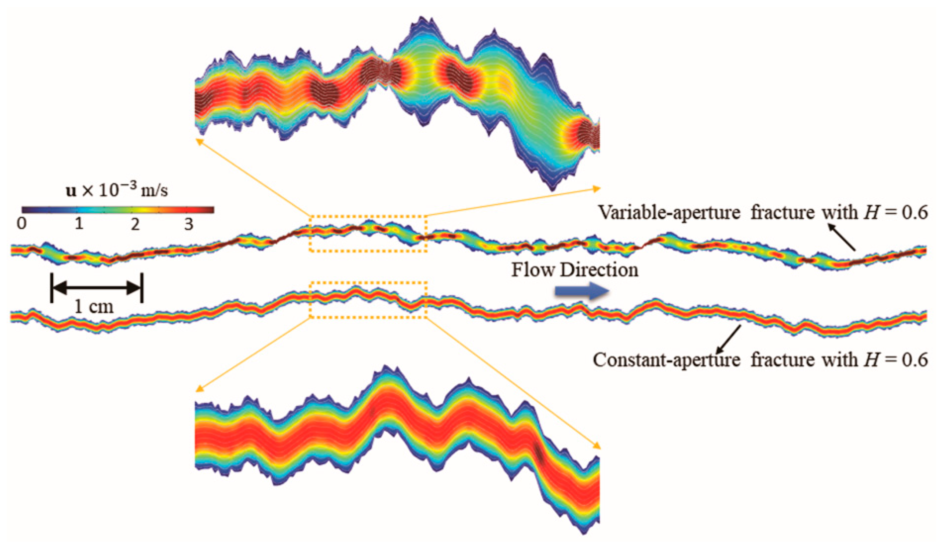
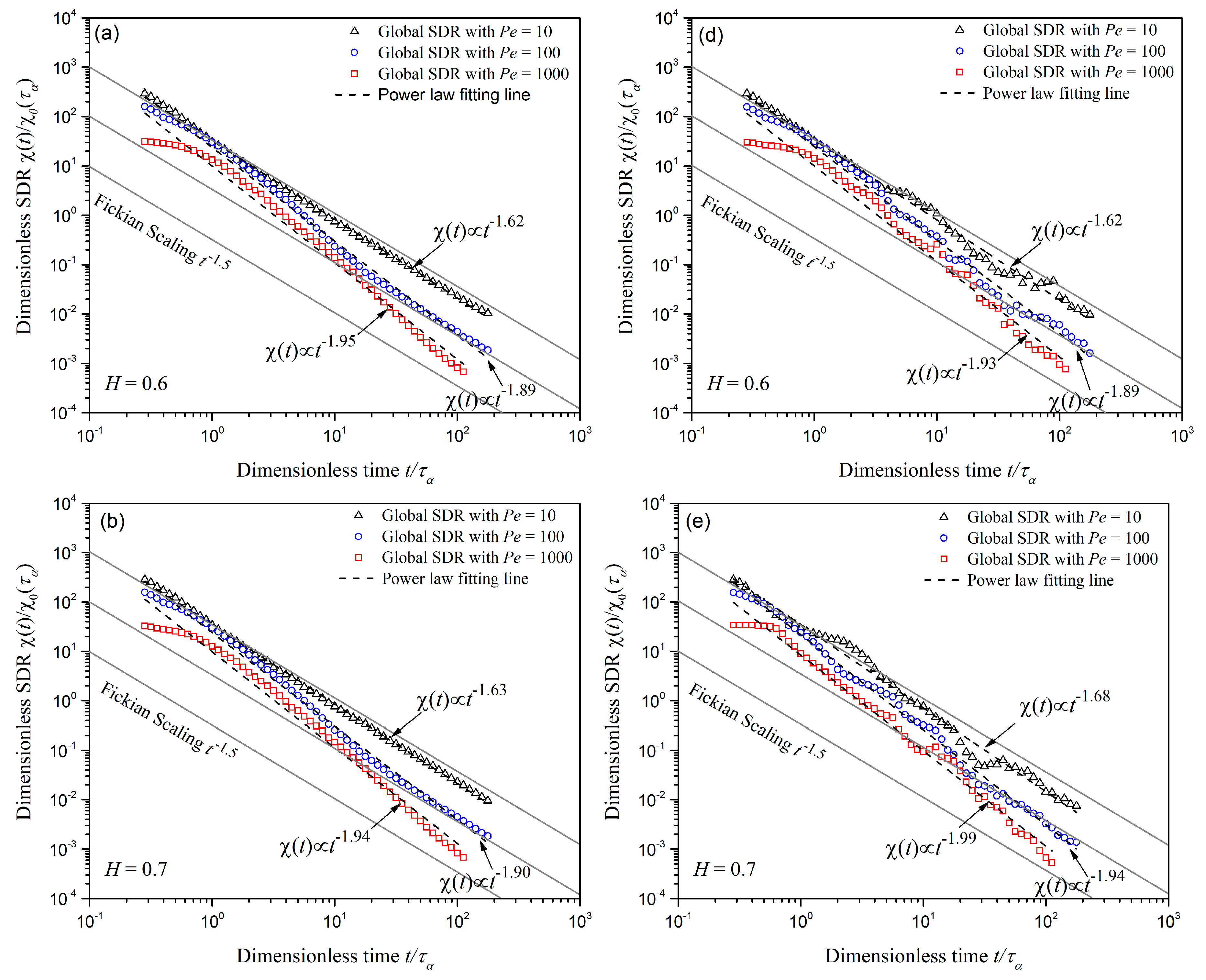
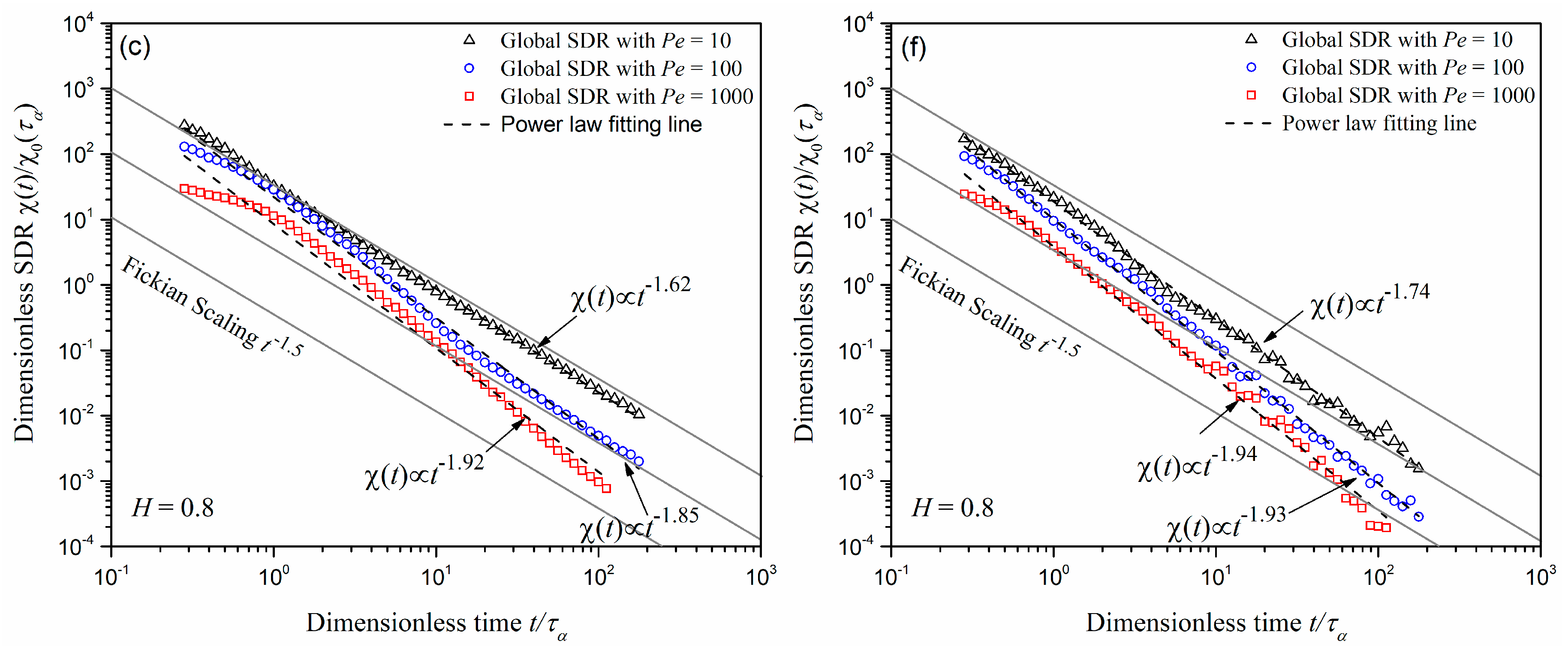
3.2. Influence of the Roughness of Fracture Walls on the Temporal Behavior of the Global SDR

To investigate the influence of the roughness of fracture walls on the temporal behavior of the global SDR, the conservative solute transport in self-affine rough fractures with different Hurst exponents and Peclet number values were simulated. Figure 6 shows the evolution of SDR in the constant-aperture fracture and variable-aperture fracture for Hurst exponents of 0.6, 0.7, and 0.8 and Peclet number values of 10, 100, and 1000. In Figure 6, the time is normalized by the characteristic advection time ${\tau }_a$ and the temporal SDR $\chi \left(t\right)$ is normalized by ${\chi }_0\left({\tau }_a\right)$. It can be seen from Figure 6 that the SDR in general decreases with time for all conditions considered. The temporal evolution of the SDR in the variable-aperture fracture fluctuates more than that in the constant-aperture fracture. This indicates that the spatial distribution of local apertures and the corresponding spatial changes in velocity have a significant influence on the temporal evolution of the SDR. Since mixing is the only process of solute mass exchange between the different streamlines, the distribution of streamlines significantly impacts the mixing [8]. In the constant-aperture fracture, the streamlines are uniform over the entire fracture, whereas the streamlines in the variable-aperture fracture are deformed and bent due to the spatial distribution of local apertures (see Figure 4). The deformed and bent streamlines lead to changes in the transverse concentration gradients during transport along the fracture. In contrast, in the constant-aperture fractures, the transverse concentration gradients are smoothed out by diffusion after the characteristic diffusion time (i.e., $>{\overline{b}}^2/D_m$). In addition, the trend in the temporal evolution of the SDR for the variable-aperture fractures reveals that the magnitude of this fluctuation is affected by the Hurst exponent. For the smaller Hurst exponents (H = 0.6 and H = 0.7), the fluctuation of the SDR around the corresponding power-law fitting line exists over the entire interval of the transport time. However, the fluctuation is much less when H = 0.8 for $t<10{\tau }_a$.

Each SDR in Figure 6 was fitted with a power-law function of the dimensionless time over the entire temporal range (${10}^{-1}<t/{\tau }_a<{10}^3$). For both constant-aperture and variable-aperture fractures, the SDR scaling for a given Peclet number is generally independent of the Hurst exponent of the fracture wall, while the Peclet number has a significant influence on the SDR scaling. When the Hurst exponent ranges from H = 0.6 to H = 0.8 the exponents in the power law fit are very similar for a particular Peclet number value in both constant-aperture and variable-aperture fractures. For one-dimensional fractures, the analytical SDR scaling follows the Fickian scaling $\mathsf{\chi }\left(t\right)\propto t^{-1.5}$, as shown in Equation (22). Thus, as per the definition by Le Borgne et al. [31], the results in Figure 6 indicate that the SDR scaling is non-Fickian and the exponent of the best-fit power law equation for the SDR increases as the Peclet number decreases. This indicates that predicting the temporal evolution of the SDR over the entire temporal range in both constant-aperture and variable-aperture fractures using the one-dimensional analytical SDR scaling is inappropriate as this underpredicts the SDR, especially for the cases with the high Peclet number. Furthermore, it can be seen from Figure 6a–c that in constant-aperture fractures, for a given Peclet number, the results are similar for H = 0.6, H = 0.7, and H = 0.8. This implies that the roughness of the self-affine fracture walls, as characterized by Hurst exponent, is not a dominant influence on the temporal evolution of the SDR in the constant-aperture fractures. In contrast, as shown in Figure 6d–f, for a given Peclet number, the exponent of the best-fitting power law decreases as the Hurst exponent increases and spatial correlation increases.

The characteristic of the mixing can be seen from the SDR scaling over the different temporal ranges. For the cases with Pe = 10 and Pe = 100 in both constant-aperture and variable-aperture fractures, the SDR scaling is approximately Fickian at late time ($t>10{\tau }_a$), but becomes non-Fickian for the temporal range examined for Pe = 1000. The transition time between the Fickian and non-Fickian temporal evolution of the SDR is important for predicting the mixing process. Before the transition time, the temporal evolution of the SDR shows non-Fickian mixing behavior [31,49]. In constant-aperture fractures (see Figure 6a–c) the transition time increases as the Peclet number increases while the transition time is insensitive to the Hurst exponent. For the cases with Pe = 100 the corresponding transition time is equal to 30${\tau }_a$, whereas for the cases with Pe = 1000 it is more than 100${\tau }_a$. In the variable-aperture fractures, both the Hurst exponent and the Peclet number influence the transition time. It fails to capture the exact transition time for the cases with Pe = 1000 due to the limitation of fracture length scale. For a given Peclet number and Hurst exponent, the occurrence of non-Fickian mixing in fractures depends on both the aperture distribution and the fracture length scale.

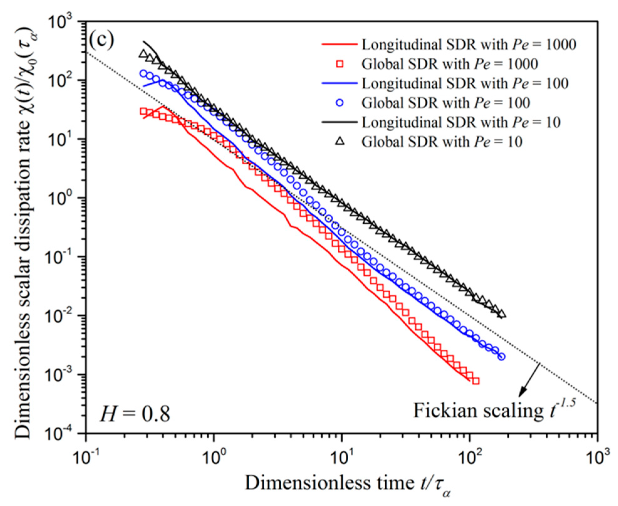
3.3. Validity of Predicting Global SDR from the Longitudinal SDR

Since Taylor’s work [23,50] demonstrated that solute transport in an asymmetrical shear flow field can be reduced to a one-dimensional dispersion process by using a longitudinal effective dispersion coefficient, this idea has been proven useful and effective among a wide range of fields and applications [37,51,52,53,54]. The spatially variable velocity field dominates the behavior of solute spreading process, while the local diffusion process can smooth concentration gradients at the same time. These two coupled processes lead to the incomplete mixing inside the plume and reflect the fact that the mixing can be considered as a result of both the local diffusion and solute spreading. Le Borgne et al. [31] pointed out that the incomplete mixing inside the plume, which generates the concentration gradients in the transverse direction, results in the non-Fickian scaling of mixing. Bolster et al. [7] distinguished the two coupled process of mixing by expressing the concentration as the sum of the average of the concentration over the transverse cross-section and the deviation about it. In order to investigate the validity of predicting the global SDR by the longitudinal SDR in both constant-aperture and variable-aperture fractures, the method in [31] was used to obtain the mean longitudinal concentration projected in the transverse direction $\overline{c}\left(x,t\right)$ and then calculate the longitudinal SDR:

$$\overline{c}\left(x,t\right)=\frac{{{\displaystyle \int }}_0^{b\left(x\right)}c\left(x,t\right)dx}{b\left(x\right)}$$

(23)

The validity of predicting the global SDR by the longitudinal SDR can be evaluated by comparing the longitudinal SDR to the global SDR. The longitudinal SDR can also be considered as the contribution of the transverse concentration gradients to the global SDR. For the cases in the constant-aperture fractures, Figure 7 shows the global SDR estimated from the full concentration field and the longitudinal SDR estimated from Equation (23). In general, regardless of the influence of the Hurst exponent and Peclet number, the temporal evolution of the longitudinal and global SDR both decrease as power-law functions of time. For the cases with Pe = 10, the longitudinal SDR is very close to the global SDR, which indicates that the longitudinal SDR is capable of predicting the global SDR in the constant-aperture fractures. This also reveals that the transverse concentration gradients, in this case, do not play a dominant role in global mixing. Thus, both of the longitudinal and global SDR follow Fickian scaling ($\mathsf{\chi }\left(t\right)\propto t^{-1.5}$).

For the cases with Pe = 100 and Pe = 1000, the longitudinal SDR is smaller than the global SDR for most of the temporal range, indicating that the longitudinal SDR underpredicts the global SDR at that time. In contrast to the cases with Pe = 10, the transverse concentration gradients are relatively large and make significant contributions to the temporal evolution of the global SDR. As the transverse concentration gradients decrease due to diffusion, the concentration distribution inside the plume becomes more homogeneous. The characteristic time for diffusion smoothing the transverse concentration gradients depends on the Peclet number. For the case with Pe = 100, the longitudinal SDR gradually converges towards the global SDR around $t/{\tau }_a=100$, which implies that the longitudinal SDR appears to be valid for predicting the global SDR when the influence of transverse concentration gradients becomes negligible. Moreover, Figure 7 shows that the Hurst exponent has little influence on the relationship between the longitudinal and the global SDR. These results indicate that in the constant-aperture fractures, the Hurst exponent is not a dominant factor in the development of transverse concentration gradients.

To predict the global SDR from the longitudinal SDR, it is essential that the temporal evolution of the longitudinal SDR has the same tendency as the global SDR, which implies that the longitudinal concentration second moment should decrease as a power-law function of time. This would be true for the cases in the constant-aperture fracture, however, it is not necessary in the variable-aperture fractures where the abruptly changing aperture leads to the convergence of streamlines. The temporal evolutions of both the longitudinal and global concentration second moments in the variable-aperture fractures were investigated. The longitudinal and global concentration second moments is associated with the temporal evolutions of longitudinal and global SDR, respectively, as shown in Figure 8. Unlike the temporal evolution of the global concentration second moment, the temporal evolution of the longitudinal concentration second moment does not follow a strictly monotonic decrease with time for all conditions considered. Consequently, the longitudinal SDR in the variable-aperture fractures has a negative value (corresponding to the discontinuities in the lines in Figure 8b,d,f) though this is not possible as per the definition of Equation (16). This negative longitudinal SDR results from the fact that the longitudinal concentration second moment increases when the plume is transported in the small-aperture regions. For conservative solute transport, the mixing is an irreversible process and associates with the entropy of the mixing system towards its maximum. Although the longitudinal SDR generally decrease as a power-law function of time in the variable-aperture fractures, the negative value in SDR is physically meaningless. Therefore, predicting the global SDR by the longitudinal SDR is inappropriate in the variable-aperture fractures.

4. Summary and Conclusions

In this work, the successive random additions technique was applied to generate the 2D self-affine fracture wall for both the variable-aperture and constant-aperture fractures. The Hurst exponent of the generated 2D fracture wall was determined by the statistical analysis of the surface heights of the dolomite rock. Although there was no contact area (zero-aperture zone) in the generated 2D fractures, the simulations of conservative solute through variable-aperture and constant-aperture fractures highlighted the influence of the Hurst exponent and Peclet number on the temporal mixing behavior. It was found that, as in porous media, the SDR, decreased as a power-law function of time, and was characteristic of the mixing in both variable-aperture and constant-aperture fractures. The Peclet number had a significant influence on the temporal evolution of the SDR. The variable-aperture distribution led to the local fluctuation of the temporal evolution of the SDR, even for the small Pe. For both the variable-aperture and constant-aperture fractures, as the Peclet number increased, the exponent of the best-fitting power law for SDR scaling decreased significantly, indicating that the relatively large Peclet number enhanced the mixing process.

The influence of Hurst exponent on the temporal evolution of the SDR was dependent on the Peclet number and the aperture distribution. For the constant-aperture fracture, the influence of Hurst exponent on the temporal evolution of the SDR become negligible when the Peclet number was relatively small. The transition time between Fickian and non-Fickian mixing process was sensitive to the Hurst exponent, Peclet number, aperture distribution, and fracture lengh scale. For a given Peclet number and Hurst exponent, the occurrence of the non-Fickian mixing in fractures was dependent on the aperture distribution and the fracture length scale.

Comparisons of the longitudinal and global SDR showed that the global SDR could be predicted from the longitudinal SDR for Peclet number values of 100 or less in the constant-aperture fracture, independent of the value of the Hurst exponent for the self-affine fracture wall. However, for Peclet number of 1000, the longitudinal SDR would overpredict the global SDR. For the variable-aperture fracture, predicting the global SDR from the longitudinal SDR was inappropriate for all Peclet number and Hurst exponents investigated due to the non-monotonic increases of the longitudinal concentration second moment, which resulted in the physically meaningless SDR (i.e., negative SDR).

This study provides new insights into the temporal mixing behavior in self-affine fractures. However, the results for the validity of predicting the global SDR from the longitudinal SDR needs to be extended and tested in 3D real fractures with a comparison with experimental data, particularly to determine the influence of contact area (zero-aperture zone) and preferential flow on the SDR. In addition, the complex flow field (i.e., turbulent flow) in fractures would have a significant influence on the temporal mixing behavior, which also needs to be considered.

References

1. Berkowitz, B.; Cortis, A.; Dentz, M.; Scher, H. Modeling non-fickian transport in geological formations as a continuous time random walk. Rev. Geophys. 2006, 44. [Google Scholar] [CrossRef]
2. Dentz, M.; Le Borgne, T.; Englert, A.; Bijeljic, B. Mixing, spreading and reaction in heterogeneous media: A brief review. J. Contam. Hydrol. 2011, 120–121, 1–17. [Google Scholar] [CrossRef] [PubMed]
3. Rolle, M.; Kitanidis, P.K. Effects of compound-specific dilution on transient transport and solute breakthrough: A pore-scale analysis. Adv. Water Resour. 2014, 71, 186–199. [Google Scholar] [CrossRef]
4. Cai, J.; Hu, X.; Xiao, B.; Zhou, Y.; Wei, W. Recent developments on fractal-based approaches to nanofluids and nanoparticle aggregation. Int. J. Heat Mass Transf. 2017, 105, 623–637. [Google Scholar] [CrossRef] [Green Version]
5. Dou, Z.; Zhou, Z.; Wang, J.; Liu, J. Pore-scale modeling of mixing-induced reaction transport through a single self-affine fracture. Geofluids 2018, 2018, 9095143. [Google Scholar] [CrossRef]
6. Liu, R.; Li, B.; Jiang, Y.; Yu, L. A numerical approach for assessing effects of shear on equivalent permeability and nonlinear flow characteristics of 2-d fracture networks. Adv. Water Resour. 2018, 111, 289–300. [Google Scholar] [CrossRef]
7. Bolster, D.; Valdés-Parada, F.J.; LeBorgne, T.; Dentz, M.; Carrera, J. Mixing in confined stratified aquifers. J. Contam. Hydrol. 2011, 120–121, 198–212. [Google Scholar] [CrossRef] [PubMed]
8. Chiogna, G.; Cirpka, O.A.; Herrera, P.A. Helical flow and transient solute dilution in porous media. Trans. Porous Media 2016, 111, 591–603. [Google Scholar] [CrossRef]
9. Dentz, M.; Carrera, J. Mixing and spreading in stratified flow. Phys. Fluids 2007, 19, 017107. [Google Scholar] [CrossRef]
10. Dreuzy, J.-R.D.; Carrera, J. On the validity of effective formulations for transport through heterogeneous porous media. Hydrol. Earth Syst. Sci. 2016, 20, 1319–1330. [Google Scholar] [CrossRef] [Green Version]
11. Kapoor, V.; Kitanidis, P.K. Concentration fluctuations and dilution in aquifers. Water Resour. Res. 1998, 34, 1181–1193. [Google Scholar] [CrossRef] [Green Version]
12. Kitanidis, P.K. The concept of the dilution index. Water Resour. Res. 1994, 30, 2011–2026. [Google Scholar] [CrossRef]
13. Le Borgne, T.; Dentz, M.; Villermaux, E. Stretching, coalescence, and mixing in porous media. Phys. Rev. Lett. 2013, 110, 204501. [Google Scholar] [CrossRef] [PubMed]
14. Rolle, M.; Eberhardt, C.; Chiogna, G.; Cirpka, O.A.; Grathwohl, P. Enhancement of dilution and transverse reactive mixing in porous media: Experiments and model-based interpretation. J. Contam. Hydrol. 2009, 110, 130–142. [Google Scholar] [CrossRef] [PubMed]
15. Tartakovsky, A.M.; Tartakovsky, G.D.; Scheibe, T.D. Effects of incomplete mixing on multicomponent reactive transport. Adv. Water Resour. 2009, 32, 1674–1679. [Google Scholar] [CrossRef]
16. Cirpka, O.A.; Kitanidis, P.K. Characterization of mixing and dilution in heterogeneous aquifers by means of local temporal moments. Water Resour. Res. 2000, 36, 1221–1236. [Google Scholar] [CrossRef] [Green Version]
17. Dou, Z.; Zhou, Z.-F.; Wang, J.-G. Three-dimensional analysis of spreading and mixing of miscible compound in heterogeneous variable-aperture fracture. Water Sci. Eng. 2016, 9, 293–299. [Google Scholar] [CrossRef]
18. Cirpka, O.A. Choice of dispersion coefficients in reactive transport calculations on smoothed fields. J. Contam. Hydrol. 2002, 58, 261–282. [Google Scholar] [CrossRef]
19. Dou, Z.; Chen, Z.; Zhou, Z.; Wang, J.; Huang, Y. Influence of eddies on conservative solute transport through a 2d single self-affine fracture. Int. J. Heat Mass Transf. 2018, 121, 597–606. [Google Scholar] [CrossRef]
20. Dou, Z.; Zhou, Z.; Wang, J.; Huang, Y. Roughness scale dependence of the relationship between tracer longitudinal dispersion and peclet number in variable-aperture fractures. Hydrol. Process. 2018, 32, 1461–1475. [Google Scholar] [CrossRef]
21. Dreuzy, J.R.; Carrera, J.; Dentz, M.; Le Borgne, T. Time evolution of mixing in heterogeneous porous media. Water Resour. Res. 2012, 48, W06511. [Google Scholar] [CrossRef]
22. De Simoni, M.; Carrera, J.; Sánchez-Vila, X.; Guadagnini, A. A procedure for the solution of multicomponent reactive transport problems. Water Resour. Res. 2005, 41, 1–17. [Google Scholar] [CrossRef]
23. Aris, R. On the dispersion of a solute in a fluid flowing through a tube. Proc. R. Soc. Lond. A Math. Phys. Eng. Sci. 1956, 235, 67–77. [Google Scholar] [CrossRef]
24. Detwiler, R.L.; Rajaram, H.; Glass, R.J. Solute transport in variable-aperture fractures: An investigation of the relative importance of Taylor dispersion and macrodispersion. Water Resour. Res. 2000, 36, 1611–1625. [Google Scholar] [CrossRef] [Green Version]
25. Freyberg, D.L. A natural gradient experiment on solute transport in a sand aquifer: 2. Spatial moments and the advection and dispersion of nonreactive tracers. Water Resour. Res. 1986, 22, 2031–2046. [Google Scholar] [CrossRef]
26. Rolle, M.; Hochstetler, D.; Chiogna, G.; Kitanidis, P.K.; Grathwohl, P. Experimental investigation and pore-scale modeling interpretation of compound-specific transverse dispersion in porous media. Trans. Porous Media 2012, 93, 347–362. [Google Scholar] [CrossRef]
27. Chiogna, G.; Hochstetler, D.L.; Bellin, A.; Kitanidis, P.K.; Rolle, M. Mixing, entropy and reactive solute transport. Geophys. Res. Lett. 2012, 39. [Google Scholar] [CrossRef] [Green Version]
28. Rolle, M.; Chiogna, G.; Hochstetler, D.L.; Kitanidis, P.K. On the importance of diffusion and compound-specific mixing for groundwater transport: An investigation from pore to field scale. J. Contam. Hydrol. 2013, 153, 51–68. [Google Scholar] [CrossRef] [PubMed]
29. Miralles-Wilhelm, F.; Gelhar, L.W. Stochastic analysis of oxygen-limited biodegradation in heterogeneous aquifers with transient microbial dynamics. J. Contam. Hydrol. 2000, 42, 69–97. [Google Scholar] [CrossRef]
30. Kapoor, V.; Gelhar, L.W. Transport in three-dimensionally heterogeneous aquifers: 1. Dynamics of concentration fluctuations. Water Resour. Res. 1994, 30, 1775–1788. [Google Scholar] [CrossRef]
31. Le Borgne, T.; Dentz, M.; Bolster, D.; Carrera, J.; de Dreuzy, J.-R.; Davy, P. Non-fickian mixing: Temporal evolution of the scalar dissipation rate in heterogeneous porous media. Adv. Water Resour. 2010, 33, 1468–1475. [Google Scholar] [CrossRef]
32. Engdahl, N.B.; Ginn, T.R.; Fogg, G.E. Scalar dissipation rates in non-conservative transport systems. J. Contam. Hydrol. 2013, 149, 46–60. [Google Scholar] [CrossRef] [PubMed] [Green Version]
33. Jha, B.; Cueto-Felgueroso, L.; Juanes, R. Quantifying mixing in viscously unstable porous media flows. Phys. Rev. E 2011, 84, 066312. [Google Scholar] [CrossRef] [PubMed]
34. Cardenas, M.B.; Slottke, D.T.; Ketcham, R.A.; Sharp, J.M. Navier-stokes flow and transport simulations using real fractures shows heavy tailing due to eddies. Geophys. Res. Lett. 2007, 34. [Google Scholar] [CrossRef]
35. Cardenas, M.B.; Slottke, D.T.; Ketcham, R.A.; Sharp, J.M. Effects of inertia and directionality on flow and transport in a rough asymmetric fracture. J. Geophys. Res. 2009, 114. [Google Scholar] [CrossRef] [Green Version]
36. Wang, L.; Cardenas, M.B. Non-fickian transport through two-dimensional rough fractures: Assessment and prediction. Water Resour. Res. 2014, 50, 871–884. [Google Scholar] [CrossRef]
37. Wang, L.; Cardenas, M.B. An efficient quasi-3d particle tracking-based approach for transport through fractures with application to dynamic dispersion calculation. J. Contam. Hydrol. 2015, 179, 47–54. [Google Scholar] [CrossRef] [PubMed]
38. Kang, P.K.; Brown, S.; Juanes, R. Emergence of anomalous transport in stressed rough fractures. Earth Planet. Sci. Lett. 2016, 454, 46–54. [Google Scholar] [CrossRef] [Green Version]
39. Mandelbrot, B.B. The Fractal Geometry of Nature; Macmillan: San Francisco, CA, USA, 1983; Volume 173. [Google Scholar]
40. Dou, Z.; Zhou, Z.; Sleep, B.E. Influence of wettability on interfacial area during immiscible liquid invasion into a 3d self-affine rough fracture: Lattice boltzmann simulations. Adv. Water Resour. 2013, 61, 1–11. [Google Scholar] [CrossRef]
41. Mondal, P.K.; Sleep, B.E. Colloid transport in dolomite rock fractures: Effects of fracture characteristics, specific discharge, and ionic strength. Environ. Sci. Technol. 2012, 46, 9987–9994. [Google Scholar] [CrossRef] [PubMed]
42. Tatone, B.S.; Grasselli, G. A method to evaluate the three-dimensional roughness of fracture surfaces in brittle geomaterials. Rev. Sci. Instrum. 2009, 80, 125110. [Google Scholar] [CrossRef] [PubMed]
43. Develi, K.; Babadagli, T. Quantification of natural fracture surfaces using fractal geometry. Math. Geol. 1998, 30, 971–998. [Google Scholar] [CrossRef]
44. Wang, J.S.Y.; Narasimhan, T.N.; Scholz, C.H. Aperture correlation of a fractal fracture. J. Geophys. Res. Solid Earth 1988, 93, 2216–2224. [Google Scholar] [CrossRef]
45. Liu, R.; Jiang, Y.; Jing, H.; Yu, L. Nonlinear flow characteristics of a system of two intersecting fractures with different apertures. Processes 2018, 6, 94. [Google Scholar] [CrossRef]
46. Bolster, D.; Dentz, M.; Le Borgne, T. Hypermixing in linear shear flow. Water Resour. Res. 2011, 47. [Google Scholar] [CrossRef] [Green Version]
47. Li, Y.-H.; Gregory, S. Diffusion of ions in sea water and in deep-sea sediments. Geochim. Cosmochim. Acta 1974, 38, 703–714. [Google Scholar]
48. Comsol, A. Comsol Multiphysics User’s Guide; Version 5.2; COMSOL Inc.: Stockholm, Sweden, 2015; Volume 10, p. 333. [Google Scholar]
49. Werth, C.J.; Cirpka, O.A.; Grathwohl, P. Enhanced mixing and reaction through flow focusing in heterogeneous porous media. Water Resour. Res. 2006, 42, 1165–1173. [Google Scholar] [CrossRef]
50. Taylor, G. Dispersion of soluble matter in solvent flowing slowly through a tube. Proc. R. Soc. Lond. A Math. Phys. Eng. Sci. 1953, 219, 186–203. [Google Scholar] [CrossRef]
51. Bouquain, J.; Méheust, Y.; Bolster, D.; Davy, P. The impact of inertial effects on solute dispersion in a channel with periodically varying aperture. Phys. Fluids 2012, 24, 083602. [Google Scholar] [CrossRef] [Green Version]
52. Briggs, S.; Karney, B.W.; Sleep, B.E. Numerical modeling of the effects of roughness on flow and eddy formation in fractures. J. Rock Mech. Geotech. Eng. 2017, 9, 105–115. [Google Scholar] [CrossRef]
53. Jin, Y.; Dong, J.; Zhang, X.; Li, X.; Wu, Y. Scale and size effects on fluid flow through self-affine rough fractures. Int. J. Heat Mass Transf. 2017, 105, 443–451. [Google Scholar] [CrossRef]
54. Dou, Z.; Zhou, Z.-F. Lattice boltzmann simulation of solute transport in a single rough fracture. Water Sci. Eng. 2014, 7, 277–287. [Google Scholar]
Figure 1. Dolomite rock fracture surface 3D profile and distribution of Hurst exponent for the different 2D profiles along the longitudinal direction.
Processes 06 00158 g001
Figure 2. Self-affine fracture walls with the different Hurst exponents. (a) The self-affine fracture walls with H = 0.6, H = 0.7, and H = 0.8, respectively. (b) The zoom-in self-affine fracture wall with H = 0.6 between x = 80 mm and x = 90 mm.
Processes 06 00158 g002
Figure 3. Reconstruction of aperture field in the self-affine rough fracture with H = 0.7. (a) Reconstruction of constant-aperture rough fracture. (b) Reconstruction of variable-aperture rough fracture. (c) Gaussian distribution of aperture field for the variable-aperture rough fracture.
Processes 06 00158 g003
Figure 4. The flow fields in variable-aperture and constant-aperture fractures with H = 0.6 for Pe = 1000.
Processes 06 00158 g004
Figure 5. The solute transport in variable-aperture and constant-aperture fractures with H = 0.6 for Pe = 1000.
Processes 06 00158 g005
Figure 6. Scalar dissipation rate estimated in the constant-aperture fracture (ac) and variable-aperture fracture (df) with H = 0.6, 0.7, and 0.8 for Pe = 10, 100, and 1000, respectively.
Processes 06 00158 g006aProcesses 06 00158 g006b
Figure 7. The global SDR estimated from the full concentration field and the longitudinal SDR estimated from the average of the concentration over the transverse cross-section in the constant-aperture fractures with the Hurst exponent H = 0.6 (a), H = 0.7 (b), and H = 0.8 (c) for the Pe = 10, 100, and 1000.
Processes 06 00158 g007aProcesses 06 00158 g007b
Figure 8. (a,c,e) represent the global concentration second moment estimated from the full concentration field and the longitudinal concentration second moment estimated from the average of the concentration over the transverse cross-section in the variable-aperture fractures with H = 0.6, H = 0.7, and H = 0.8, respectively. (b,d,f) represent the global SDR estimated from the full concentration field and the longitudinal SDR estimated from the average of the concentration over the transverse cross-section in the variable-aperture fractures with the Hurst exponent H = 0.6, H = 0.7, and H = 0.8 for the Pe = 10, 100, and 1000, respectively.
Processes 06 00158 g008