Numerical Investigation of the Failure Mechanism of Transversely Isotropic Rocks with a Particle Flow Modeling Method

Abstract

Transversely isotropic rocks are commonly encountered in rock engineering practices, and their strength and failure behavior is often governed by the property of anisotropy. The particle flow modeling method was utilized to investigate the failure mechanism of transversely isotropic rocks subject to uniaxial compressive loading. The details for establishing transversely isotropic rock models were first presented, and then a parametric study was carried out to look into the effect of interface properties on the failure mode and strength of transversely isotropic rock models by varying the interface dip angle. The smooth joint model was incorporated to create interfaces for the completeness of establishing transversely isotropic rock models with the particle flow modeling method. Accordingly, three failure modes observed in transversely isotropic rock models with varying dip angles were tensile failure across interfaces, shear failure along interfaces, and tensile failure along interfaces. Furthermore, the interface mechanical parameters were found to differently influence the failure behavior of transversely isotropic rock models. The bonded joint cohesion and bonded joint friction angle that contribute to the shear strength of interfaces have considerable influence on the uniaxial compressive strength (UCS) values, while the joint coefficient of friction and joint tensile strength have a slight influence on the UCS values. The findings in this paper indicated the importance of interfaces in estimating failure behavior of transversely isotropic rocks.

1. Introduction

The dominant anisotropy or transverse isotropy of geological materials, especially of foliated metamorphic rocks, such as slates, gneisses, schist, and sedimentary rocks with bedding planes, leads to complicated failure behaviors [1]. Rock anisotropy is one of the most significant characteristics that should be taken into consideration for underground engineering. The design and stability analysis of underground structures excavated in anisotropic rock masses, for instance, require a complete understanding of the failure behavior of the rock materials. Thus, the failure mechanism of anisotropic or transversely isotropic rocks has been a significant topic in rock mechanics.

Engineering practice has suggested that the rock anisotropy is of importance in the stabilization of underground excavations in bedded rock masses [2,3]. Previous studies indicate that drilling through bedding planes was quite dangerous. The boreholes might become unstable if the deviation angle of drilled well applied to sub-horizontal bedding planes is very high due to rock strength anisotropy [4,5,6,7,8]. Particularly, Okland et al. [4] carried out hollow cylinder tests to study the critical bedding inclination angle of shale that can induce severe borehole damage during extended reach drilling. Meier et al. [6] also claimed that the lowest stress is required to induce borehole breakout when the borehole is sub-parallel to the bedding planes. Moreover, Zhou et al. [9] reported that in the Wudongde hydropower station on the Jinsha River in China, instability of high sidewalls, particularly separation of bedding planes and the accompanying remarkable deformation, is likely to happen in those sections where strata are almost parallel to the cavern axis with a thickness less than 10 cm. For better engineering design, the mechanical properties of aforementioned anisotropic rock materials are suggested to be determined through the field tests or through rock mass classification [10].

However, due to the inherent difficulty and inaccuracy in conducting field tests or rock mass classification, many investigators tend to investigate the mechanical properties of anisotropic rock materials through laboratory tests. To be specific, Gatelier et al. [11], according to laboratory tests, stated a decrease in uniaxial compressive strength with increasing inclination angle in Adamswiller sandstone. Kim et al. [12] through X-ray CT (Computed Tomography) study and uniaxial compression tests found that Berea sandstone in northern Ohio is composed of cross-bedded loose layers and relatively thin tightly packed layers, and its uniaxial compressive strength (UCS) value decreases with increasing porosity as well as with increasing inclination of the bedding plane. Heng et al. [13] investigated the directional shale samples obtained from the Longmaxi Formation in Shizhu County, China, and three types of shear failure modes were identified that were dependent on the shearing angle, which were sliding failure across the bedding plane, sliding failure along the bedding planes, and sliding failure across the bedding planes combined with tensile splitting along the bedding planes. Besides these real rock materials prepared from engineering sites, some rock-like materials have also been utilized to investigate the anisotropic or transversely isotropic mechanism. Kulatilake et al. [14] carried out uniaxial compressive tests on the jointed rock-like material blocks having existing joint sets. Their findings show that for rock samples with dip angles of 0° to 15°, the failure mechanism was the tensile failure through the intact model material, while for rock samples with joint dip angles of 40° to 60°, the main failure mechanism was the combined shear and tensile failure through the joints. A mixed mechanism of the above two modes accounted for the failure of jointed blocks having dip angles of 20° to 35°. Yang et al. [15] performed a series of physical model tests for jointed rock masses with persistent discontinuities and indicated that the failure modes of these models with different dip angles can be divided into split mode, sliding mode, and mixed mode. Recently, an experimental investigation was implemented by Yang et al. [16] on jointed rock models made of rock-like materials. In accordance with the experimental results, the failure of simulated rock models with varied orientations is classified into one of four modes: (a) tensile failure across the joint plane, (b) shear failure along the joint plane, (c) tensile failure along the joint plane, and (d) intact material failure. These above-mentioned researchers explained the anisotropic or transversely isotropic mechanism of rock materials with weak planes/layers presence. These studies broaden our understanding of weak planes/layers geometry on the mechanical property of rock materials.

As one important research methodology in rock mechanics as well as in geotechnical engineering, the numerical modeling method has significantly enriched the data bank of anisotropic rock behavior besides those obtained from laboratory experiments. Particularly, the particle flow modeling method with the basis of the discrete element theory has obtained a pronounced development from being applied to rock and soil mechanics to greatly broader applications. This approach is capable of deriving the rock mass response based on the relatively simple particle contact laws at joints and in rock instead of more complex constitutive models [17,18]. Therefore, a particle flow modeling approach could be utilized directly to extend the experimental results obtained in the laboratory. For example, Chiu et al. [19] put forward a modified smooth-joint model utilizing the particle flow modeling approach to mimic the anisotropic behavior of a rock mass, and the failure modes of the rock mass obtained by Yang et al. [15] in the laboratory were perfectly reproduced. The load-deformation curves in different joint orientations were also well mimicked. Bahaaddini et al. [18], by using particle flow modeling, thoroughly investigated the effect of geometric parameters of joints on the rock mass failure mechanism, deformation modulus, and uniaxial compression strength, and critically compared these with the physical experiments [20]. Park and Min [21] also conducted particle flow simulations with embedded smooth joints for mimicking the strength and failure behavior of transversely isotropic rocks with systematic verification and extensions to laboratory and field problems. They succeeded in capturing the failure modes observed in anisotropic rock in which weak planes significantly matter. Furthermore, the particle flow modeling has been utilized as well to study the failure behavior of transversely isotropic rock mass through Brazilian tests [1,22]. Although the particle flow modeling promotes the understanding of the anisotropic or transversely isotropic rock mass mechanical behavior, the concentration is still mainly put on the geometrically structural effect. On the other hand, the influence of bedded planes/layers’ mechanical properties on the failure response of anisotropic or transversely isotropic rock masses is not well understood.

This study aims to better understand the influence of mechanical properties of bedded layers (interfaces) on the failure behavior of transversely isotropic rocks through a particle flow modeling method. Thus, this paper is organized in the following matter. First, the physical experiment on simulated transversely isotropic rocks is briefly introduced in Section 2.1 as a benchmark for particle flow modeling. After that, the procedure to establish particle flow models, which consists of intact materials and interfaces, and the calibration of their mechanical parameters, are illustrated in Section 2.2. With these numerically simulated models, the failure mechanism of transversely isotropic rocks is analyzed at the mesoscale under uniaxial compressive loading in Section 3.1. In Section 3.2, a sensitivity study is carried out systematically to estimate the influence of mechanical parameters of interfaces on the failure strength of transversely isotropic rocks.

2. Materials and Methods

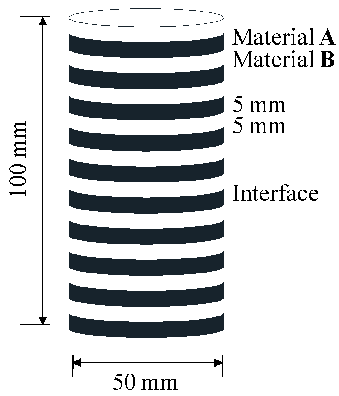
2.1. Physical Experiment on Simulated Transversely Isotropic Rocks

To investigate the failure mechanism of the transversely isotropic rocks through particle flow modeling, associated experimental results are required. The present modeling study refers to artificial transversely isotropic rocks, as implemented by Tien et al. [23], and utilized their test data for the base of the particle flow simulations. The physical experiment program and results are described as follows.

Two model materials, referred to as material A and material B, respectively, were chosen to combine into the transversely isotropic rock samples. Material A was composed of cement, kaolinite, and water in a weight ratio of 4:1:1.2, while material B was composed of cement, kaolinite, and water in a weight ratio of 1:1:0.6. According to the test results of the materials’ mechanical properties, the uniaxial compressive strength (UCS), Young’s modulus, and Poisson’s ratio of material A are 104.2 MPa, 21.7 GPa, and 0.23, respectively, representing rocks with high strength and stiffness. On the other hand, the uniaxial compressive strength, Young’s modulus, and Poisson’s ratio of material B are 43.3 MPa, 11.9 GPa, and 0.21, respectively, representing rocks with relatively low strength and stiffness.

Tien et al. [23] incorporated eight steps to develop these transversely isotropic rock samples. After the mold assembly and model material preparation steps (steps 1 and 2), the preliminary compaction step (step 3) was conducted by using the MTS (Mechanical Testing and Simulation) servo-controlled loading frame to apply an axial load of 20 kN on the model materials to make them into a preliminary square rock mass soft enough for cutting into slices. In the cutting into slices step (step 4), the preliminarily compacted model materials (material A and material B) were put on a cutting platform and cut with a slice cutter into slices with a thickness of 5 mm in each layer. After that, a suction lifter was utilized to pile material A slices and material B slices up in sequence, which is referred to as the stacking slices step (step 5). Following the repairing step (step 6), the final compaction step (step 7) was implemented to apply a final load of 114 kN on those sliced materials, and then it was held for one hour until a steady settlement was achieved. Finally, upon the curing and drilling step (step 8), the transversely isotropic rock samples having different dip angles (α = 0°, 15°, 30°, 45°, 60°, 75°, and 90°) were created for the subsequent compression tests. These artificial transversely isotropic rock samples were developed to represent the anisotropic behavior of sandstone-shale interlayered rock masses. Figure 1 shows the physical dimension of a typical transversely isotropic rock sample.

These artificial transversely isotropic rock samples were then subjected to compression tests. In accordance with the test results [23], with zero confining pressure, three failure modes were identified. When the dip angles were relatively low (α = 0°, 15°, and 30°), the artificial transversely isotropic rock samples failed in a mode of tensile fracture across discontinuities; whereas, when the dip angles were medium (α = 45°, 60°, and 75°), the artificial transversely isotropic rock samples failed in a mode of sliding failure along discontinuities. Moreover, for artificial transversely isotropic rock sample having a vertical dip angle, its failure mode was defined as the tensile-split along discontinuities.

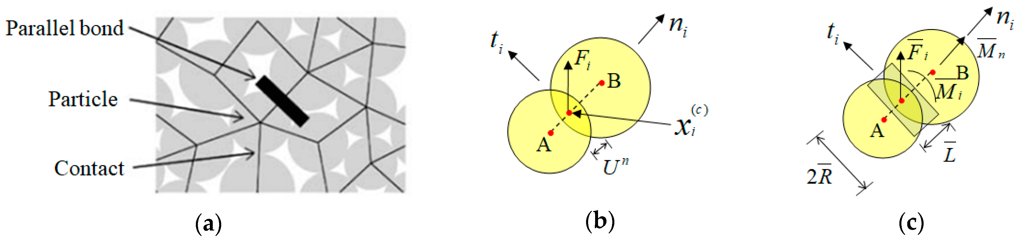
2.2. Particle Flow Modeling of Material A and Material B

The particle flow code in three dimensions (PFC^3D) is a commercial software package based on the discrete element method [24,25]. In this study, PFC^3D was utilized to develop the particle flow models of transversely isotropic rocks. In PFC^3D, the intact materials (material A and material B) were mimicked through a composite of particles that interact with each other at contacts (Figure 2a). A linear contact model provides an elastic relationship between the relative displacements and forces of particles at the point contact (Figure 2b). This model consists of the contact normal force component, $F_n$, contact overlap, $U_n$, shear increment, $\Delta F_s$, and shear displacement increment, $\Delta U_s$, as follows:

$$F_n=k_n{U}_n$$

(1)

$$\Delta F_s=-k_s\Delta U_s$$

(2)

with $k_n$ and $k_s$ being the contact normal and shear stiffness.

The frictional resistance of the contact is as follows:

$$F_s\le \mu F_n$$

(3)

with $\mu$ being the friction coefficient between particles.

To numerically mimic a relatively rock-like material, it is required to stick these granular particles through a bonded model [26]. The bonded model, herein, is a parallel bond model that resists not only the contact forces but also the moments between the particles at a cemented contact (Figure 2c). The function mechanism of the parallel bond model is described as:

$$\Delta {\overline{F}}_n={\overline{k}}_{n}A\Delta U_n$$

(4)

$$\Delta {\overline{F}}_s=-{\overline{k}}_{s}A\Delta U_s$$

(5)

and

$$\Delta {\overline{M}}_n=-{\overline{k}}_{s}J\Delta {\theta }_n$$

(6)

$$\Delta {\overline{M}}_s=-{\overline{k}}_{n}I\Delta {\theta }_s$$

(7)

with ${\overline{F}}_n$, ${\overline{F}}_s$, ${\overline{M}}_n$, and ${\overline{M}}_s$ being the force components and moments about the center of the cemented-contact zone, respectively; ${\overline{k}}_n$ and ${\overline{k}}_s$ being the normal and shear bond stiffness per unit area, respectively; ${\theta }_n$ and ${\theta }_s$ being the rotation angle components, respectively; and A, J, and I being the area, polar moment of inertia, and moment of inertia of the bond contact cross-section, respectively. The strength value of the bonded contact is given by:

$${\overline{\sigma }}_{\max }=\frac{-{\overline{F}}_n}{A}+\frac{\left|{\overline{M}}_s\right|\overline{R}}{I}<{\overline{\sigma }}_c$$

(8)

$${\overline{\tau }}_{\max }=\frac{-{\overline{F}}_s}{A}+\frac{\left|{\overline{M}}_n\right|\overline{R}}{J}<{\overline{\tau }}_c$$

(9)

with $\overline{R}$ being the radii of the cemented contact plane between particles (Figure 2c); and ${\overline{\sigma }}_c$ and ${\overline{\tau }}_c$ being the tensile and shear strength of the bond contact, respectively.

Tensile cracks occur when the applied normal stress exceeds the specified tensile strength of the parallel bond, ${\overline{\sigma }}_c$, while shear cracks happen as the applied shear stress surplus the shear strength, ${\overline{\tau }}_c$, either through rotation or through sliding of particles. The tensile strength at the contact soon falls to zero once the cracks occur, while the shear strength decreases as the residual friction strength (Equation (3)).

For presenting the aforesaid mechanical properties of material A and material B, this numerical modeling method requires a calibration of the microparameters to describe contact and bond deforming and strength behavior, and the selected package of microparameters are expected to derive the macro mechanical properties of simulated material used in physical experiments [23]. Therefore, a calibration procedure was carried out to determine these microparameters for intact rock materials (material A and material B). Several steps [25,27,28,29] are followed to reproduce certain properties of the artificial materials. First, the particle and parallel bond moduli and the ratios of normal to shear stiffness are set to be equal between the particles and parallel bonds, which aims to decrease the number of independent parameters. Second, the Young’s modulus is determined through setting the material strengths to a large value and varying E_c (particle Young’s modulus) and ${\overline{E}}_c$ (parallel bond Young’s modulus) to match the Young’s modulus between the particle flow modeling and laboratory samples (with the size of φ 50 mm × 100 mm). Then, through varying $k_n/k_s$ (particle normal stiffness/shear stiffness) and ${\overline{k}}_n/{\overline{k}}_s$ (parallel bond normal stiffness/shear stiffness), the Poisson’s ratio of the intact synthetic cylindrical sample was matched to the laboratory samples. Afterwards, the strength between the numerical and laboratory samples were matched by decreasing the normal and shear bond strengths of the parallel bonds. During this procedure, it is of importance to fix the ratio of normal to shear bond strength (${\overline{\sigma }}_c/{\overline{\tau }}_c$) for the reason that it influences the failure pattern of the sample. The determined microparameters of the intact rock material were listed in

Table 1. Microparameter values of intact rock materials (material A and material B).

Property	Parameter	Value1 (Material A)	Value2 (Material B)
Particle	$\rho$ (kg/m3)	2150	1760
	$k_n/k_s$	1.65	1.55
	$E_c$ (GPa)	18.8	10.3
	μ	0.554	0.466
	$R_{rat}=R_{\max }/R_{\min }$	1.66	1.66
	Rmin (mm)	0.65	0.65
Parallel bond	$\lambda$	1.0	1.0
	${\overline{k}}_n/{\overline{k}}_s$	1.65	1.55
	${\overline{E}}_c$ (GPa)	18.8	10.3
	${\overline{\sigma }}_c$ (mean ± std.dev., MPa)	76.0 ± 19.0	31.7 ± 7.9
	${\overline{\tau }}_c$ (mean ± std.dev., MPa)	152.0 ± 38.0	63.4 ± 15.9

Note that $\rho$ is the density of the synthetic rock material; $\lambda$ is the radius multiplier used to set the parallel bond radii; $R_{rat}$ is the radius of the particle; $R_{\max }$ and $R_{\min }$ are the maximum radius and minimum radius of the particle, respectively.

. A comparison between particle flow modeling and experiment results in

Table 2. Comparison of mechanical properties of intact material between the physical experiment and the particle flow modeling results.

Material	Macro Properties	Experimental Results	Numerical Results	Abs. Deviation
Material A	UCS (MPa)	104.2	105.8	1.53%
	E (GPa)	21.7	20.8	4.15%
	ν	0.230	0.224	2.61%
Material B	UCS (MPa)	43.3	44.1	1.85%
	E (GPa)	11.9	11.4	4.20%
	ν	0.210	0.202	3.81%

claims a good capability of this numerical modeling method to reproduce these simulated mechanical properties under uniaxial compression loading. The deviations for uniaxial compressive strength (UCS), Young’s modulus (E), and Poisson’s ratio (ν) of material A and material B were all less than 5.0%.

2.3. Particle Flow Modeling of Interface between Material A and Material B

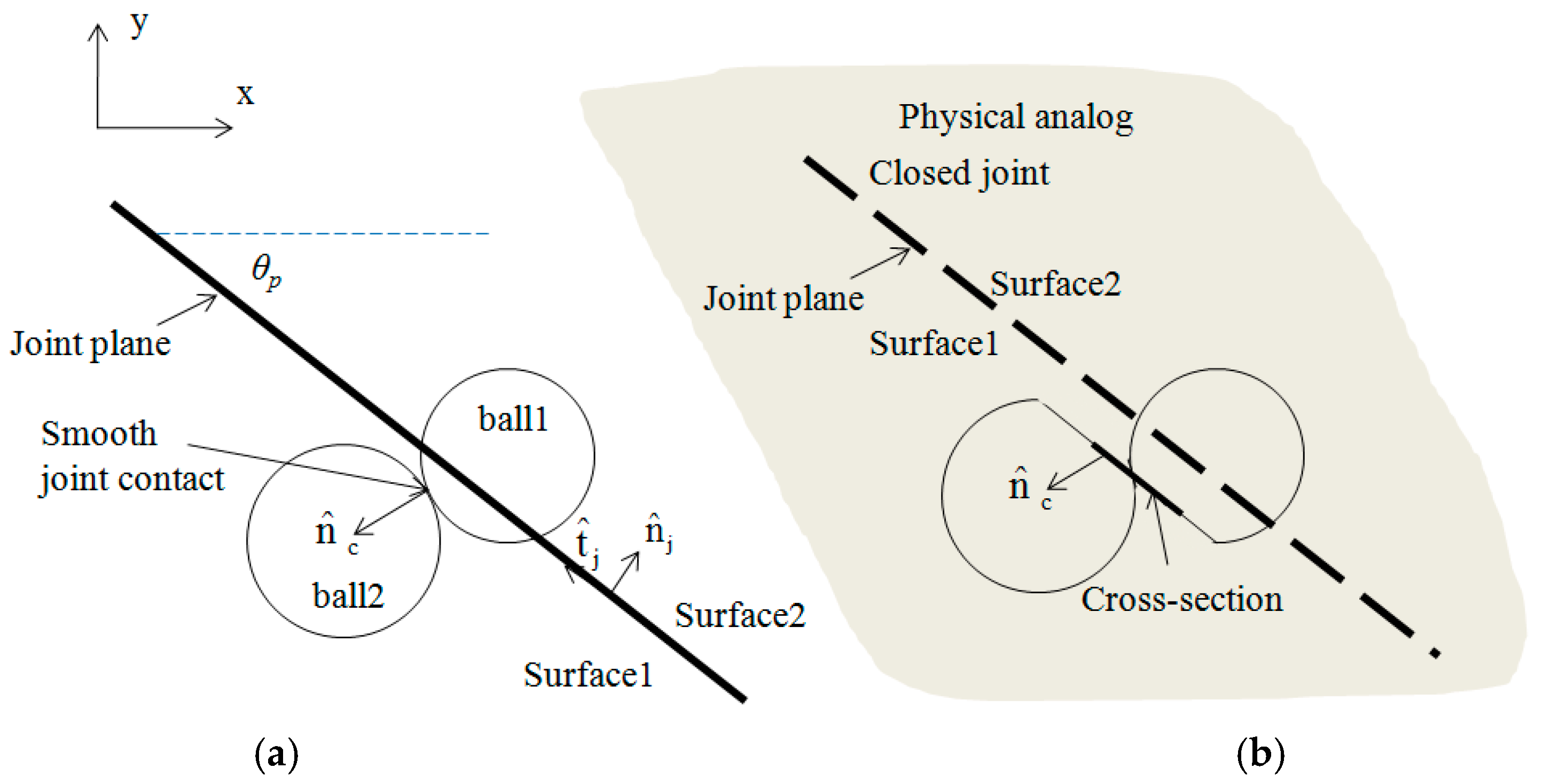
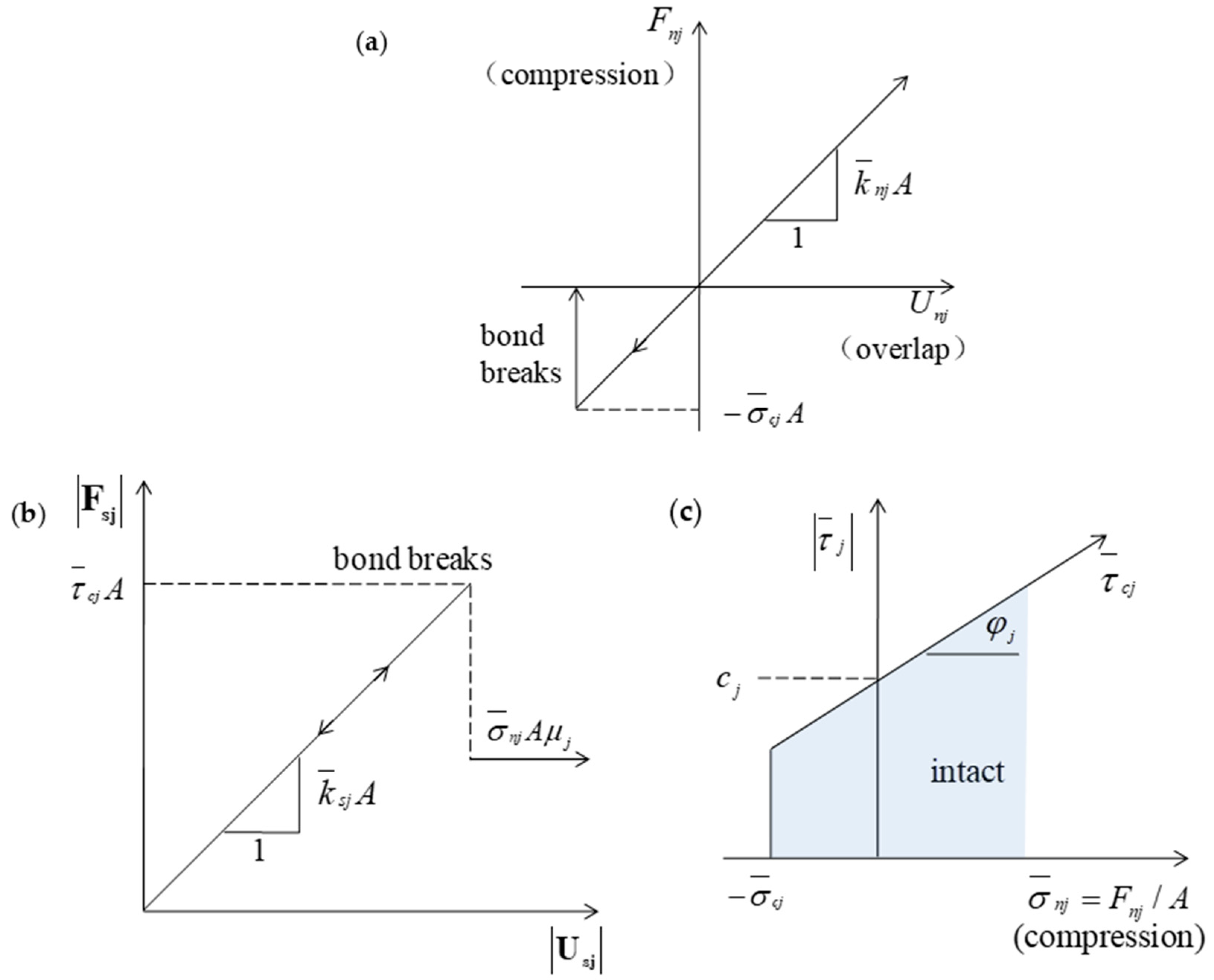
2.3.1. Smooth Joint Model

As aforementioned, the simulated transversely isotropic rock samples were prepared through piling up the material A slices and material B slices in sequence [23]. The interfaces between material A and material B (as shown in Figure 1) were discontinuities that behave quite differently from the adjacent intact materials. Hence, to better describe the mechanical behavior of transversely isotropic rocks the interfaces were intersected between material A and material B slices and represented with the smooth joint model. The numerically developed transversely isotropic rock samples having different interface dip angles are shown in Figure 3.

The smooth joint model is shown in Figure 4. Once a joint plane is defined, a smooth joint is defined at contacts between the particles whose centers are lying on the opposite sides of the joint plane. At the contacts, the existing parallel bonds will be removed first, and the smooth joints are assigned in the direction parallel to the joint plane. These contacts will act in accordance with the rules defined through the smooth joint model with particular parameter values assigned by the user. The particles having such contacts may overlap or overpass through each other rather than to roll around one another (Figure 4).

The newly defined contacts act mechanically like a set of elastic springs uniformly distributed on a circular cross-section disc with the center at the contact point. The area A of the smooth joint disc is defined as:

$$A=\pi {\overline{R}}^2$$

(10)

where $\overline{R}$ is the disc radius:

$$\overline{R}=\lambda \min (R_1,R_2)$$

(11)

where $\lambda$ is a radius multiplier (usually set as 1.0), and $R_1$ and $R_2$ are particle radii, as shown in Figure 4.

The smooth joint model can behave with respect to the following basic modes: (i) not bonded and never fail mode, (ii) not bonded and fail in tension mode, (iii) not bonded and fail in shear mode, and (iv) bonded mode. Through these modes, the smooth joint model could be used to simulate various discontinuity conditions. In the present paper, we use the smooth joint model with the bonded mode (mode (iv)) to mimic the interfaces between material A slices and material B slices. Besides the stiffness provided by the aforementioned springs, the bonded smooth joint model also possesses both the normal and shear strengths. The shear strength is given by:

$${\overline{\tau }}_{cj}={\overline{\sigma }}_{nj}\tan {\phi }_j+c_j$$

(12)

In Equation (12), ${\overline{\sigma }}_{nj}$ implies the normal stress acted on the joint surface; ${\phi }_j$ implies the bonded joint friction angle; while $c_j$ implies the bonded joint cohesion, given in MPa. If the normal or shear stress exceeds the corresponding bond strength, the joint bond between the joint surfaces fails and the bond stiffness will be removed. As long as the joint bond fails either in shear or tensile pattern, the shear strength reduces as its residual value and the tensile strength will be set to be zero. The residual shear strength is a function of the normal stress, ${\overline{\sigma }}_{nj}$, as well as the joint friction coefficient, ${\mu }_j$. Figure 5 shows the constitutive law for the bonded smooth joint model.

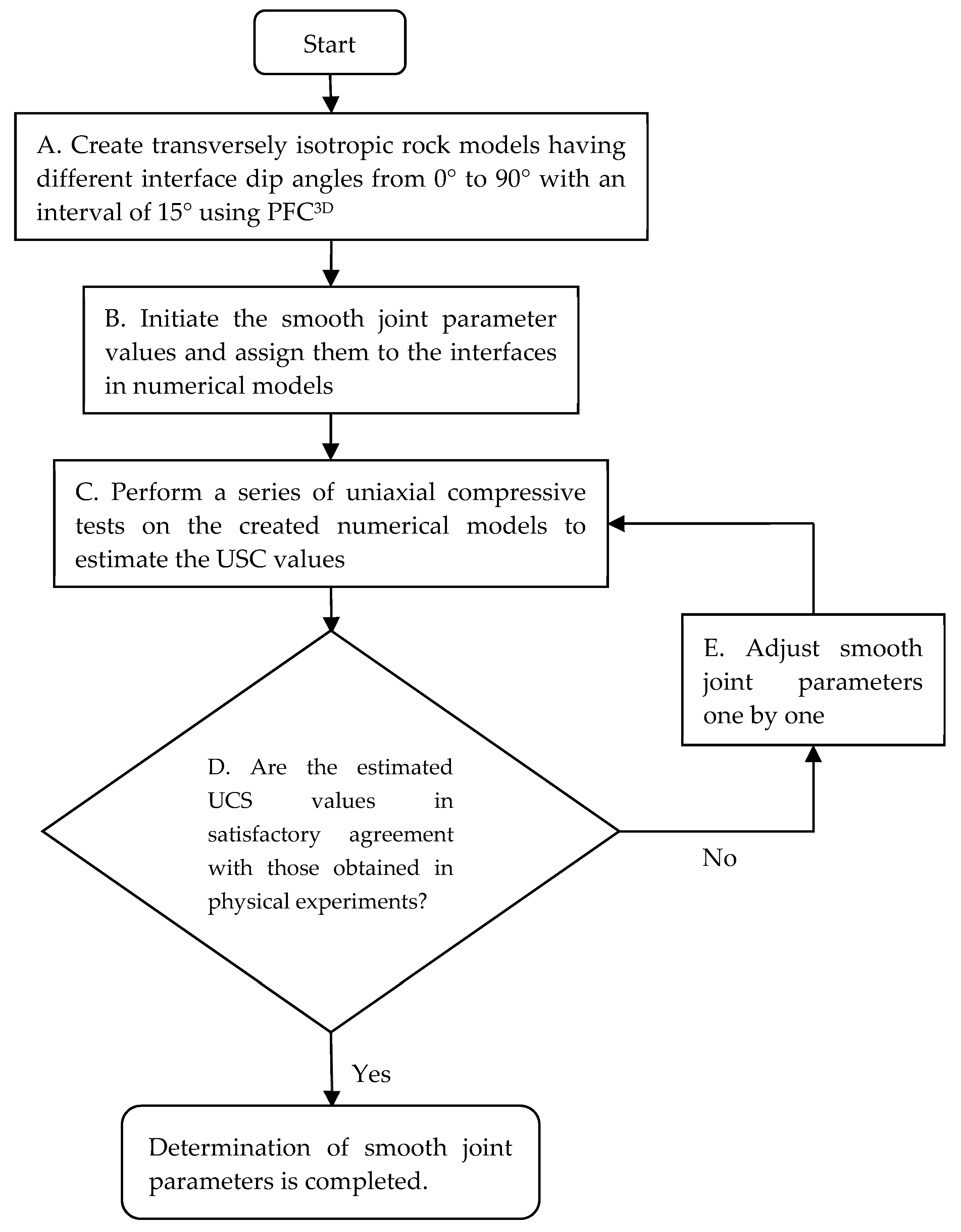
2.3.2. Calibration and Validation of Smooth Joint Mechanical Parameters

The smooth joint parameters consist of the joint normal stiffness, ${\overline{k}}_{nj}$; joint shear stiffness, ${\overline{k}}_{sj}$; joint tensile strength, ${\overline{\sigma }}_{cj}$; joint shear strength, ${\overline{\tau }}_{cj}$; joint coefficient of friction, ${\mu }_j$; and joint dilation angle, ${\psi }_j$. These mechanical parameters have been determined through a calibration procedure utilizing the data of experiments carried out by Tien et al. [23] on simulated transversely isotropic rock samples. The calibration process is illustrated in Figure 6. During the calibration procedure, sets of trial-and-error tests were implemented on numerically developed transversely isotropic rock samples (Figure 3) to reproduce the uniaxial compressive strength data with those obtained by Tien et al. [23].

Through the above calibration procedure, the mechanical parameters of the smooth joint model for simulating interfaces are determined as listed in

Table 3. Mechanical parameter values used for the smooth joint model.

Mechanical Parameter	Determined Value	Mechanical Parameter	Determined Value
${\overline{k}}_{nj}$ (N/m³)	1.81 × 1012	${\overline{\sigma }}_{cj}$ (MPa)	23.8
${\overline{k}}_{sj}$ (N/m³)	0.79 × 1012	$c_j$ (MPa)	13.0
${\mu }_j$	0.78	${\phi }_j$	22.5°
$\psi$	0	-	-

. Note that the value for each smooth joint parameter is not unique. That is to say, each joint parameter in Table 3 is changeable along with re-adjusting other joint parameters. Strong coupling effects exist between various joint parameters such that the macro mechanical properties of the simulated transversely isotropic rock models is a result of the complicated interaction among these joint parameters [30]. Based on the calibrated smooth joint mechanical parameters, the UCS of transversely isotropic rock samples are matched well with those obtained by Tien et al. [23].

Table 4. Comparison of UCS values between physical experiment and numerical simulation results.

Comparison Condition	UCS Value for Different Interface Dip Angle
Dip angle, α (deg.) Physical experiment (MPa)	0 53.0	15 47.0	30 50.0	45 38.0	60 30.0	75 38.0	90 66.0
Numerical simulation (MPa)	51.6	56.8	51.5	36.7	32.0	36.2	52.4

shows a comparison of unconfined strength values (UCS) between the experiments and the particle flow simulations. The comparison given claims the capability of the particle flow modeling method to derive the strength property of transversely isotropic rock models under uniaxial compressive loading. The uniaxial compressive strength values obtained through particle flow simulations agree well with those obtained through physical experiments. The particle flow models with the determined intact material and smooth joint mechanical parameters are subsequently utilized to investigate the failure mechanism of transversely isotropic rocks.

3. Results and Discussion

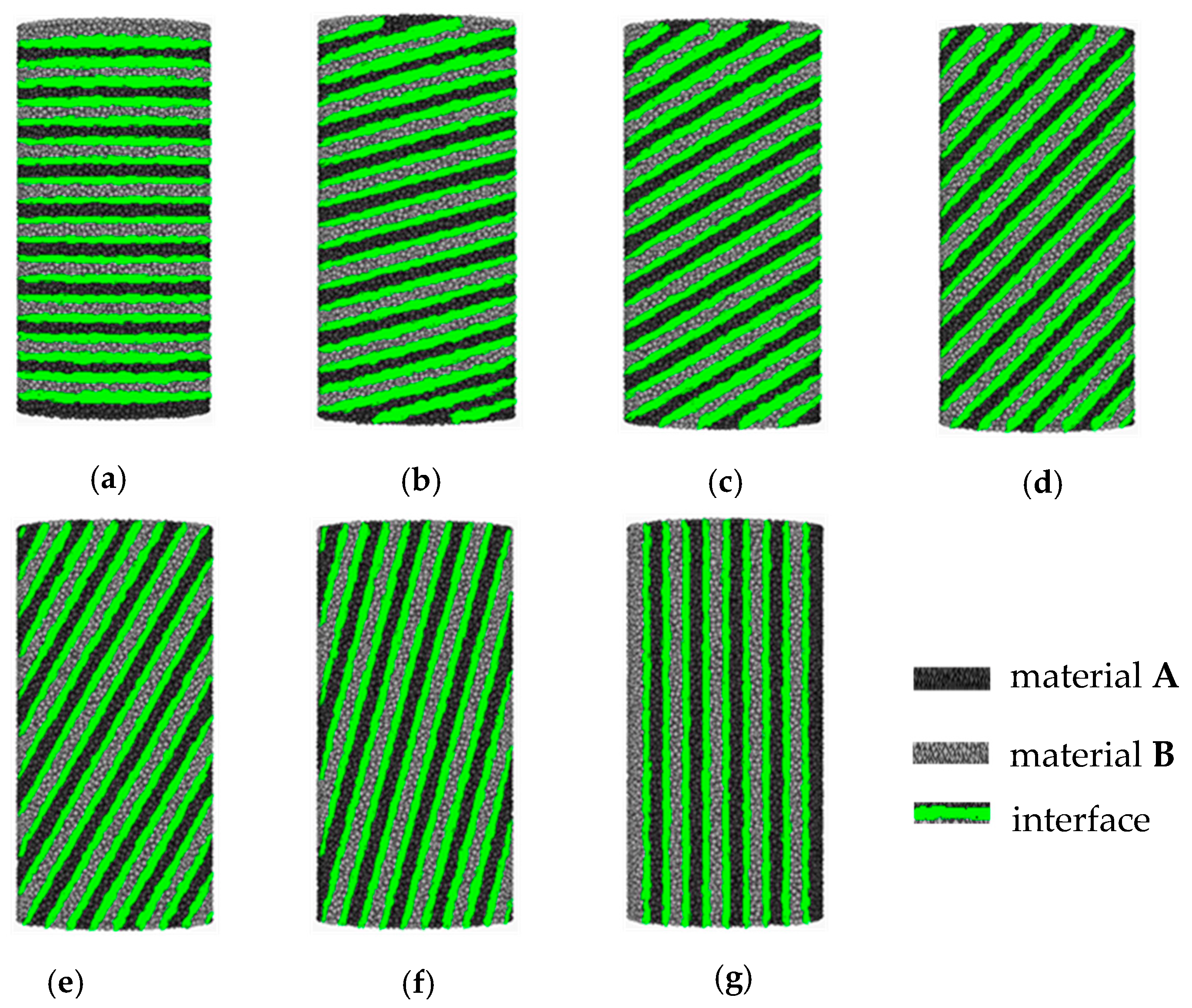
3.1. Failure Mechanism of Transversely Isotropic Rocks

For better understanding of the failure mechanism of transversely isotropic rocks under uniaxial compressive loading, the created particle flow models, of which the mechanical parameters are determined through the above calibration procedure, were investigated under differing interface dip angles. The interface dip angles were varied from 0° to 90° with an interval of 15°. In this section, failure modes of transversely isotropic rock models are analyzed in terms of newly generated cracks which present the breakage of parallel bonds as well as the smooth joint bonds. Figure 7 plots the failure process of transversely isotropic rock models having different interface dip angles. Note that the breakage of parallel bonds is shown as red (tensile) or blue (shear) crack items, whereas the breakage of smooth joint bonds is marked as magenta (tensile) or black (shear) crack items. As shown in Figure 7, when the interface dip angles, α, are 0° and 15°, under uniaxial compressive loading the cracks initiate in the soft material (material B) rather than in the hard material (material A). With subsequent compression, the cracks (tensile and shear) increasingly occur both in material A and material B, and eventually coalesce into a macro failure plane penetrating the transversely isotropic rock models. This macro failure plane comes across the simulated interfaces, the rock models fail, and resistance capability was lost. At α = 30°, the cracks also initiated in material B under uniaxial compressive loading, as shown in Figure 7. With increasing compression stress, the cracks develop not only in intact materials (material A and material B), but also in interfaces. As a result, the final failure planes were generated along the soft intact material as well as the interfaces. At α = 45°, although considerable cracks developed in the soft intact material and interfaces, the failure planes that penetrated and failed the whole rock samples only occurred along the interfaces. When the interface dip angle increased to 60° and 75°, similar failure processes were observed, as shown in Figure 7, and the final failure planes were generated along the interfaces. When the beddings were vertical (α = 90°), numerous cracks occurred both in material A and material B, and were mainly concentrated in the top and bottom ends of the simulated rock sample at the final stage.

Figure 8 shows a comparison of the failure modes of artificial and simulated transversely isotropic rock samples with dip angles of 0°, 15°, and 30°. This figure shows that the numerically simulated failure modes matched well with those obtained by Tien et al. in the physical experiments [23]. Therefore, the numerically simulated failure modes could be referred to as tensile fractures across discontinuities as defined in physical experiments. To be more specific, in this study the failure mechanism was further analyzed at the mesoscale. Figure 9 illustrates the microcrack number evolution of transversely isotropic rock models having interface dip angles of 0°, 15°, and 30°. As shown in this figure, under uniaxial compressive loading, the crack number increased slowly at the beginning, and increased sharply when the axial stress reached the peak. Additionally, the crack number in intact materials was consistently larger than that in interfaces. That is to say, the intact materials rather than the interfaces dominated the resistance capability of the whole transversely isotropic rock models. Moreover, as shown in Figure 10, in intact materials, the tensile crack number was dramatically larger than that of shear cracks. Therefore, tensile failure of an intact material is thought to be the main cause of the transversely isotropic rock models failing when the interface dip angles are relatively low, e.g., α = 0° and 15°. Taking the effect of interfaces into consideration, this type of failure mode, herein, was redefined as the tensile failure across interfaces. As the interface dip angle increased from 0° to 30° through 15°, the difference of crack number in intact materials and in interfaces decreased, as shown in Figure 9. Furthermore, at α = 30°, the crack number in interfaces almost equaled that in interfaces. Therefore, when the interface dip angle was 30° the transversely isotropic rock sample partially fails in the mode of tensile failure across interfaces.

Figure 11 displays the comparison of failure modes of artificial and simulated transversely isotropic rock models having dip angles of 45°, 60°, and 75°. It shows that the numerically simulated failure modes were also in good agreement with those obtained through physical experiments [23]. The numerically simulated failure modes could be defined as a sliding failure along discontinuities in accordance with the physical experiments. Furthermore, Figure 12 displays the crack number evolution of transversely isotropic rock models having interface dip angles of 45°, 60°, and 75°. As shown in this figure, under compressive loading, the crack number increases slowly for a relatively long period, and increases sharply when the axial stress arrives at peak stress. Contrary to transversely isotropic rock samples having low dip angles (α = 0°, 15°, and 30°), the transversely isotropic rock samples having medium dip angles (α = 45°, 60°, and 75°) generated more cracks in interfaces than in intact materials. That is to say, the interfaces rather than the intact materials dominated the resistance capability of the whole rock models. Moreover, as shown in Figure 13, in interfaces, the shear crack number was much larger than that of the tensile crack. Therefore, the shear failure of interfaces was the main mechanism of the transversely isotropic rock models failing when the interface dip angles were medium, e.g., α = 45°, 60°, and 75°. To emphasize the failure mechanism of the transversely isotropic rock models, this type of failure mode, herein, is redefined as the shear failure along interfaces.

Figure 14 plots the comparison of failure modes of transversely isotropic rock models with vertical interfaces in numerical simulations and in physical experiments [23]. In the numerically simulated rock model, there were many more cracks observed than those in the physical rock model. This might be because the particle flow modeling method could recognize more microcracks than the eyes [18]. On the other hand, Figure 15 displays that before the peak stress, the number of interface cracks was larger than that of intact material crack, which accounts for the failure planes mainly observed in vertical interfaces of artificial rock models having a dip angle of 90°. This failure mode, herein, is referred to as tensile failure along interfaces.

3.2. Effect of Interfaces on Strength of Transversely Isotropic Rocks

As aforesaid, the role of interfaces played an influence on the failure behavior of transversely isotropic rocks. The failure mode of transversely isotropic rocks were classified into three types, which are tensile failure across interfaces, shear failure along interfaces, and tensile failure along interfaces. The failure mode are significantly dependent on the interface dip angle. However, in laboratory experiments, the interfaces between material A and material B were somehow ignored without taking their mechanical properties into account [23]. This section thus focuses on the effect of interfaces on the strength behavior of transversely isotropic rock models.

For comparison, Figure 16 displays the failure modes of transversely isotropic rock models without interfaces. This figure shows that the rock models having only inter-beddings of material A and material B still behaved anisotropically. The microcracks mainly concentrated in the soft material, i.e., material B, and most of them were tensile cracks (red), which was also observed by Kim et al. [12] through experimental tests on Berea sandstone. However, as shown in Figure 17, which illustrates the comparison of UCS of transversely isotropic rocks with and without weak interfaces, the UCS values of rock models without weak interfaces were highly beyond those obtained in physical experiments. On the contrary, the UCS values of rock models with weak interfaces agreed very well with the physical experiment results. In addition, the shape of the compressive strength interface dip angle curve obtained in physical experiments could be classified as a shoulder type [31], which means that the compressive strength was relatively high with low and high dip angles, while the compressive strength was relatively low with medium dip angles. Some typical examples of such curves are verified by Yasar [32], Autio et al. [33], Nasseri et al. [34], Cho et al. [35], and Fjaer and Nes [36]. In these studies, the research objects included various rocks such as sandstone, siltstone, shale, gneiss, and schist. In most of these works, it was noted that bedding planes acted as planes of weakness. The particle flow modeling results of transversely isotropic rocks with interfaces fit this type of the compressive strength interface dip angle curve. That is to say, the interfaces were very necessary elements to build transversely isotropic rock models with particle flow modeling method. To further understand the effect of interfaces on the failure behavior of transversely isotropic rocks, the mechanical properties of interfaces were systematically investigated as follows.

3.2.1. Joint Normal Stiffness

To look into the effect of the interface property on the failure behavior of transversely isotropic rock models, the joint normal stiffness of interfaces, ${\overline{k}}_{nj}$, was first investigated. A set of joint normal stiffness values of 0.15 × 10¹³ N/m³, 0.50 × 10¹³ N/m³, 1.50 × 10¹³ N/m³, and 5.00 × 10¹³ N/m³ were numerically tested, respectively, for the transversely isotropic rock samples having various interface dip angles from 0° to 90° with an interval of 15° (Figure 3). Meanwhile, the joint shear stiffness, ${\overline{k}}_{sj}$, was set to be $1/3{\overline{k}}_{nj}$ for all tests. Furthermore, the other smooth joint parameters were kept constant, i.e., ${\overline{\sigma }}_{cj}=23.8 \mathrm{MPa}$, ${\phi }_j=22.5°$, $c_j=13.0 \mathrm{MPa}$, and ${\mu }_j=0.40$. Due to the planar surface of the interfaces in the physical experiments, the joint dilation angle, ${\psi }_j$, was always set to be 0. Figure 18 shows the uniaxial compressive strength variation of transversely isotropic rock samples with different joint normal stiffness. It is shown that the joint normal stiffness had a dramatic effect on the uniaxial compressive strength (UCS) of transversely isotropic rocks. Particularly, when the interface dip angle was less than 30° (i.e., α = 0° and 15°), the UCS basically increased with the increment of joint normal stiffness. Whereas, when the interface dip angle was equal or more than 30° (α ≥ 30°), the UCS decreased with the increment of joint normal stiffness. Moreover, as the joint normal stiffness, ${\overline{k}}_{nj}$, was set to be 0.50 × 10¹³ N/m³, the numerically obtained set of UCS values of transversely isotropic rock samples were close to those obtained in physical experiments [23].

3.2.2. Joint Shear Stiffness

Keeping the joint normal stiffness constant (i.e., ${\overline{k}}_{nj}=0.5\times {10}^{13} \mathrm{N}/{\mathrm{m}}^3$), the joint shear stiffness, ${\overline{k}}_{sj}$, is subsequently adjusted from $1/10{\overline{k}}_{nj}$ to $1.0{\overline{k}}_{nj}$ through $1/3{\overline{k}}_{nj}$. Furthermore, the other smooth joint parameters were set to be constant, that is to say, ${\overline{\sigma }}_{cj}=23.8 \mathrm{MPa}$, ${\phi }_j=22.5°$, $c_j=13.0 \mathrm{MPa}$, and ${\mu }_j=0.40$. Figure 19 shows the UCS variation of transversely isotropic rock samples with different joint shear stiffness. As shown in this figure, the joint shear stiffness possessed a similar influence to the joint normal stiffness with respect to the UCS values of transversely isotropic rock samples. When the interface dip angle was less than 30°, the UCS basically increased with the increment of joint shear stiffness. Meanwhile, when the interface dip angle was equal to or more than 30° (α ≥ 30°), the UCS decreased with the increment of joint shear stiffness. Specially, as the joint shear stiffness, ${\overline{k}}_{sj}$, was set to be $1/3{\overline{k}}_{nj}$, the numerically obtained set of UCS values of transversely isotropic rock samples agreed well with those obtained by Tien et al. in the physical experiments [23].

The joint normal stiffness and joint shear stiffness had a similar influence on the UCS variation of transversely isotropic rock models. When the interface dip angle was low (e.g., α = 0° and 15°), the uniaxial loading compressed the inter-layered materials (material A, material B, and interfaces) to deform normally, which was dominated by the normal stiffness, and further to deform tangentially, which was dominated by the shear stiffness because of the Poisson’s ratio effect, which means that the normal deformation would induce the tangential deformation. If the joint stiffness was low, the interfaces would have a large stiffness difference compared with the adjacent intact materials (material A and material B), which resulted in a significant deforming difference between them. Figure 20 shows the force chains in the transversely isotropic rock models having horizontal interfaces (α = 0°) with different joint normal stiffness values at the peak stress. It shows that the deforming difference caused tensile force chains in the interfaces, and the lower joint stiffness (e.g., ${\overline{k}}_{nj}=0.15\times {10}^{13} {\mathrm{N}/\mathrm{m}}^3$) introduced more tensile force chains. These tensile force chains further cause tensile cracks and eventually lower the UCS values of transversely isotropic rock samples. Therefore, the UCS decreased with the reduction of joint stiffness at low dip angles (i.e., α = 0° and 15°), as shown in Figure 18 and Figure 19. On the other hand, when the interface dip angle was higher (α ≥ 30°), both the high joint stiffness and the low joint stiffness induced substantial tensile force chains in the interfaces. However, the lower joint stiffness (e.g., ${\overline{k}}_{nj}=0.15\times {10}^{13} {\mathrm{N}/\mathrm{m}}^3$) increased the deforming capability of these interfaces and postponed their failure. This process motivated more intact material to contribute to the bearing capability of the whole rock samples. Therefore, the UCS increased with the reduction of joint stiffness at higher dip angles (i.e., α ≥ 30°).

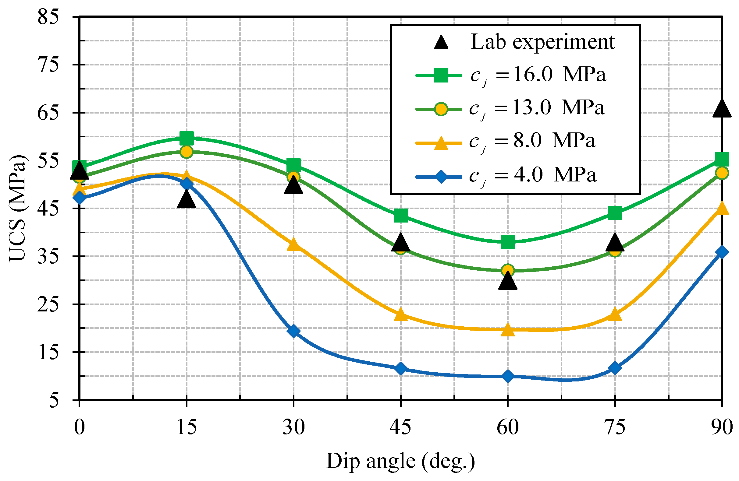
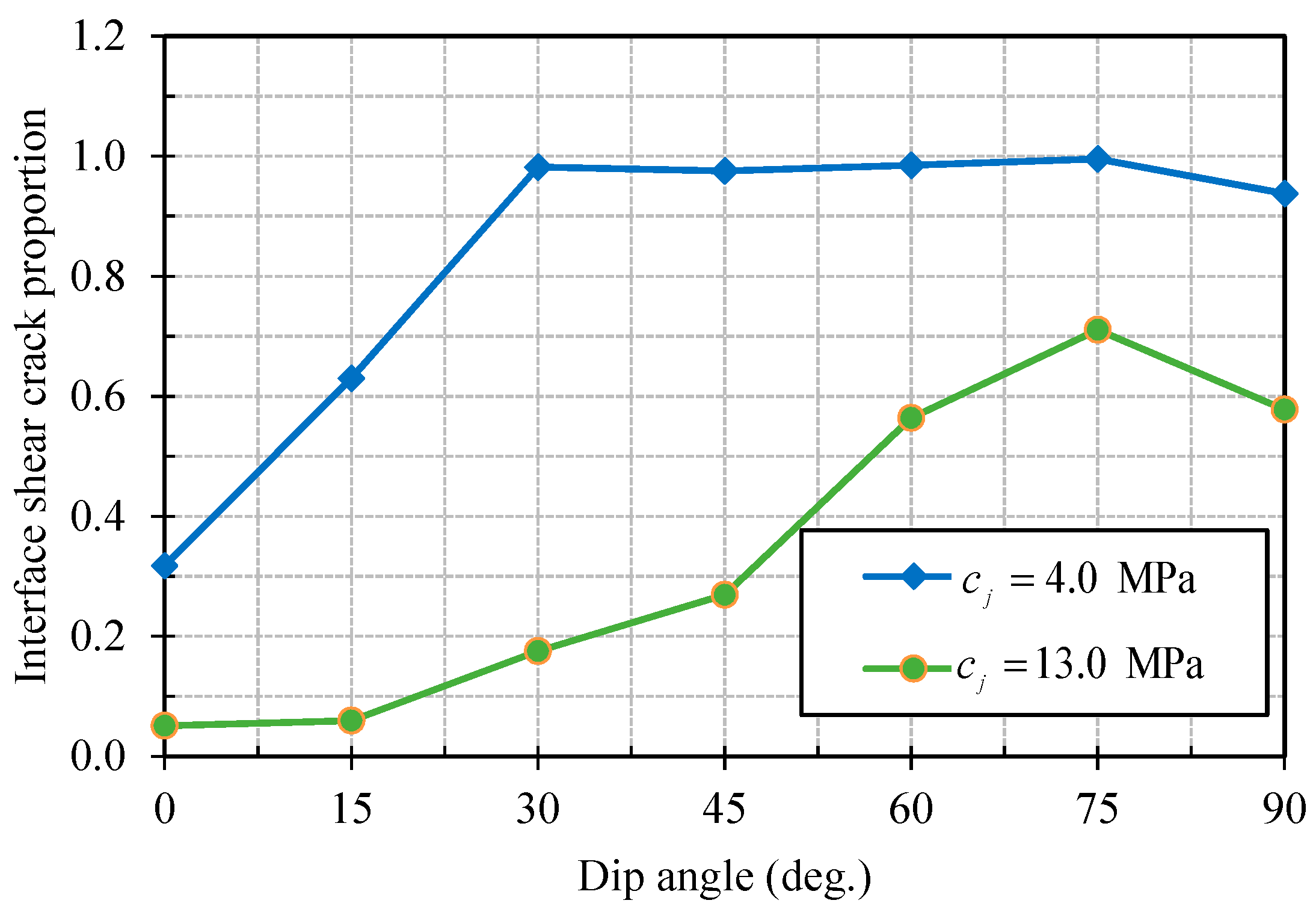
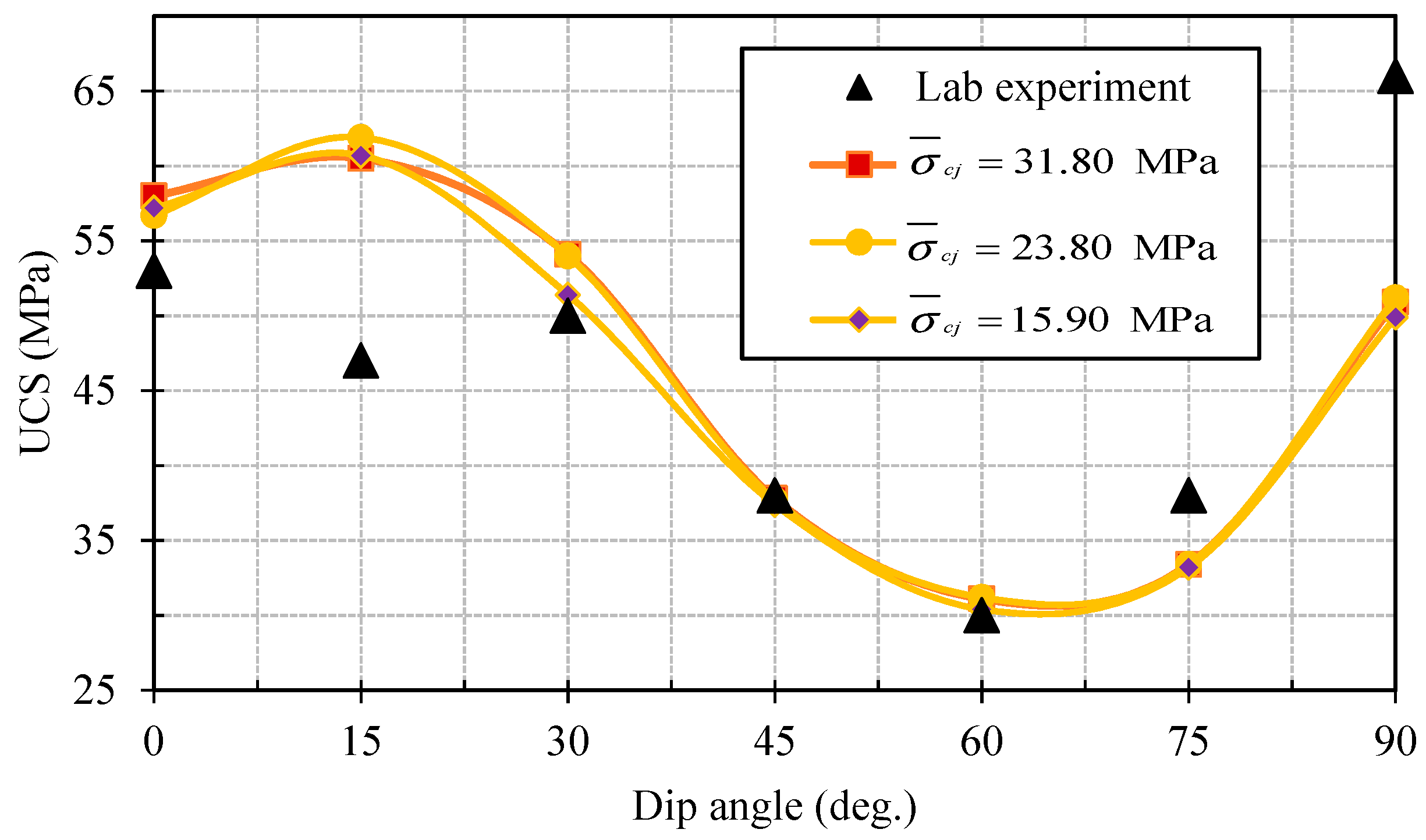
3.2.3. Bonded Joint Cohesion

Further investigation was implemented to look into the effect of interface strength parameters, including joint shear strength, ${\overline{\tau }}_{cj}$, joint coefficient of friction, ${\mu }_j$, and joint tensile strength, ${\overline{\sigma }}_{cj}$, on the strength behavior of transversely isotropic rock models. In accordance with Equation (9), the joint shear strength consisted of bonded joint cohesion, $c_j$, and bonded joint friction angle, ${\phi }_j$. Herein, the bonded joint cohesion was first adjusted to be 4.0 MPa, 8.0 MPa, 13.0 MPa, and 16.0 MPa, while the other joint parameters were kept constant, i.e., ${\overline{k}}_{nj}=0.5\times {10}^{13} \mathrm{N}/{\mathrm{m}}^3$, ${\overline{k}}_{sj}=1/3{\overline{k}}_{nj}$, ${\overline{\sigma }}_{cj}=23.8 \mathrm{MPa}$, ${\phi }_j=22.5°$, and ${\mu }_j=0.40$.

Figure 21 shows the UCS variation of transversely isotropic rock samples with different bonded joint cohesion. As shown in this figure, the bonded joint cohesion, $c_j$, had a varying influence on the UCS values depending on the interface dip angle. Specifically, when the interface dip angles, α, were 0° and 15°, the UCS values decreased slightly with the decrement of bonded joint cohesion. Even though the transversely isotropic rock samples with dip angles of 0° and 15° failed in the mode of tensile failure across interfaces (Figure 8), the shear cracks occurred in interfaces, as shown in Figure 22. This figure displays the interface shear crack proportion at peak stress varying with bonded joint cohesion of 13.0 MPa and 4.0 MPa. For a better understanding, the shear crack number in interfaces was normalized by the total crack number in the whole rock model. With the decrement of bonded joint cohesion, the shear crack number in the interfaces increased significantly. At α = 0°, when the bonded joint cohesion decreased from 13.0 MPa to 4.0 MPa, the interface shear crack proportion increased from 5.1% to 31.8%. The occurrence of more interface shear cracks accelerated the failure of the whole rock model. Moreover, at α = 15°, when the bonded joint cohesion decreased from 13.0 MPa to 4.0 MPa, the interface shear crack proportion increased from 5.9% to 63.0%. Therefore, the shear failure, in this case, became dominated when the bonded joint cohesion was small, and the failure mode changed from tensile failure across interfaces to shear failure along interfaces.

When the interface dip angles were medium (α = 30°, 45°, 60°, and 75°), the UCS values decreased heavily with the decrement of the bonded joint cohesion (Figure 21). The decrement of bonded joint cohesion directly reduced the shear resistance capability of interfaces, and made them much easier to fail. As shown in Figure 22, with the bonded joint cohesion decreasing from 13.0 MPa to 4.0 MPa, the shear cracks in the interfaces having medium dip angles were the main cracks occurring in the whole rock models. The intact materials (material A and material B) could not play their role effectively to contribute to the resistance capability of the whole models, which accounted for the decrement of UCS values in Figure 21. When the interfaces were vertical (α = 90°), even though the interface shear crack proportion increased from 57.8% to 93.8% with the bonded joint cohesion decreasing from 13.0 MPa to 4.0 MPa, the UCS value decreased less significantly, as shown in Figure 21. This was because the intact materials (material A and material B) could still resist the top and bottom loading platens moving towards each other, and even their connections (interfaces) were very weak.

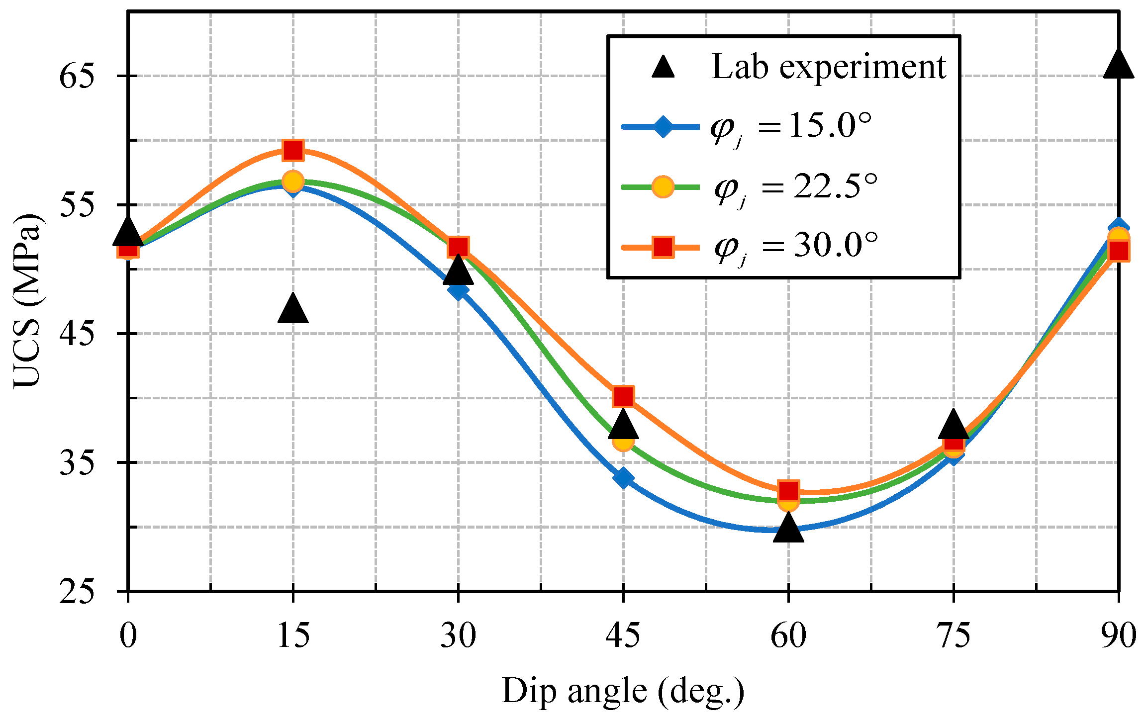
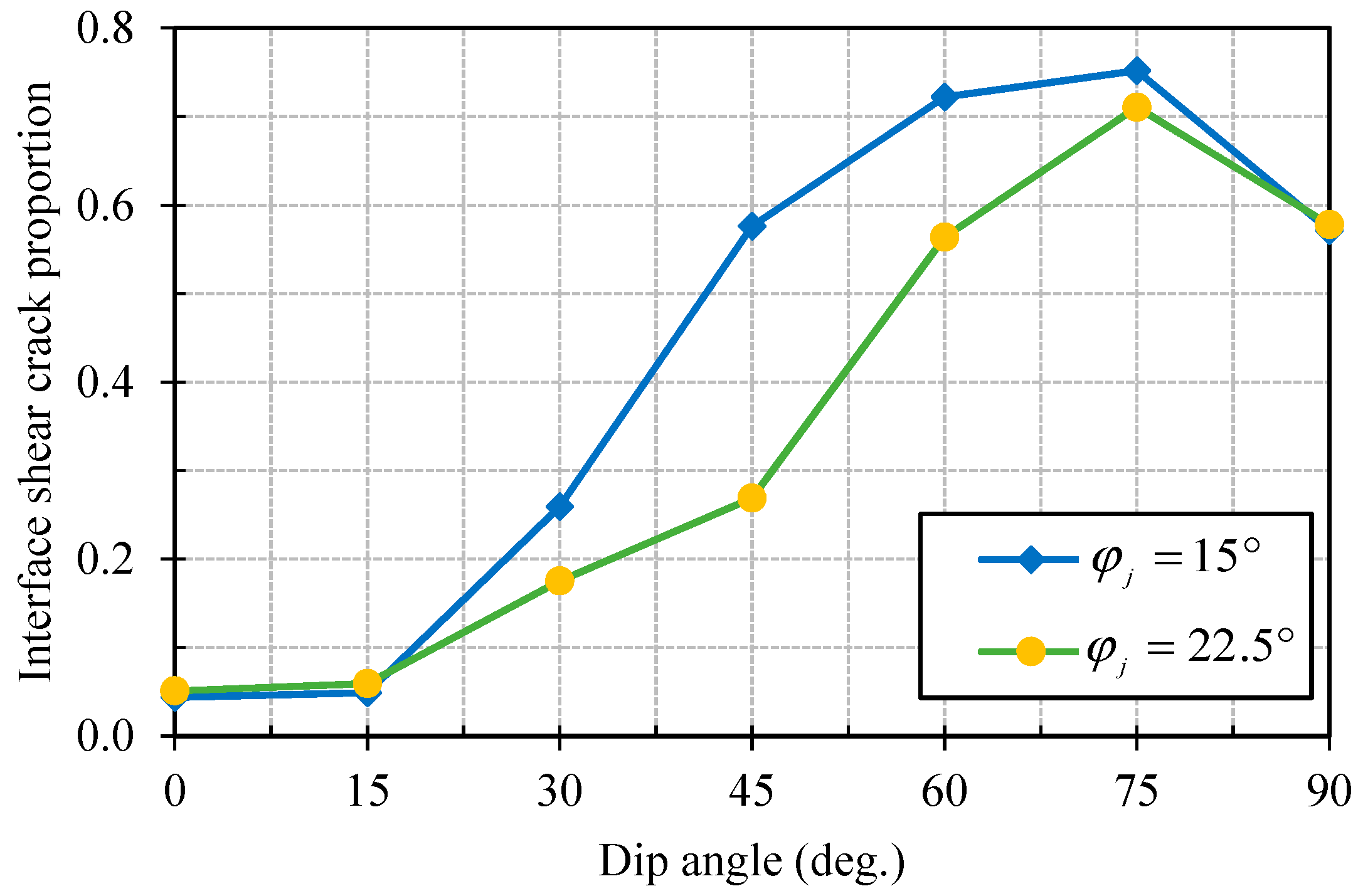
3.2.4. Bonded Joint Friction Angle

The bonded joint friction angle, ${\phi }_j$, was then adjusted to 15°, 22.5°, and 30°, respectively, while the other joint parameters were kept constant, i.e., ${\overline{k}}_{nj}=0.5\times {10}^{13} \mathrm{N}/{\mathrm{m}}^3$, ${\overline{k}}_{sj}=1/3{\overline{k}}_{nj}$, ${\overline{\sigma }}_{cj}=23.8 \mathrm{MPa}$, $c_j=13.0 \mathrm{MPa}$, and ${\mu }_j=0.40$. Figure 23 shows the UCS variation of transversely isotropic rock samples with different bonded joint friction angles. As shown in this figure, the modification of the bonded joint fiction angle had certain influences on the UCS values of transversely isotropic rock samples when the interface joint angles were medium. However, this influence was negligible when the interface was horizontal (α = 0°) or vertical (α = 90°). Like bonded joint cohesion, the bonded joint friction angle contributed to the shear strength of interfaces. However, the contribution of the bonded joint friction angle depended on the normal stress component in accordance with Equation (9). Thus, the bonded joint friction had a negligible influence on the shear resistance of the interfaces when the dip angles were high, i.e., α = 75° and 90°, due to the small normal stress component. With respect to the case of α = 0°, although the normal stress component was considerable, which enhanced the interface shear strength, the shear behavior of the interfaces was not the main mechanism for the failure of the whole rock model. This accounted for the negligible variation of the UCS values with the bonded joint friction angle at α = 0° in Figure 23. Figure 24 further indicates that the change of bonded joint friction angle mainly influenced the failure behavior of transversely isotropic rock samples when the dip angles were medium.

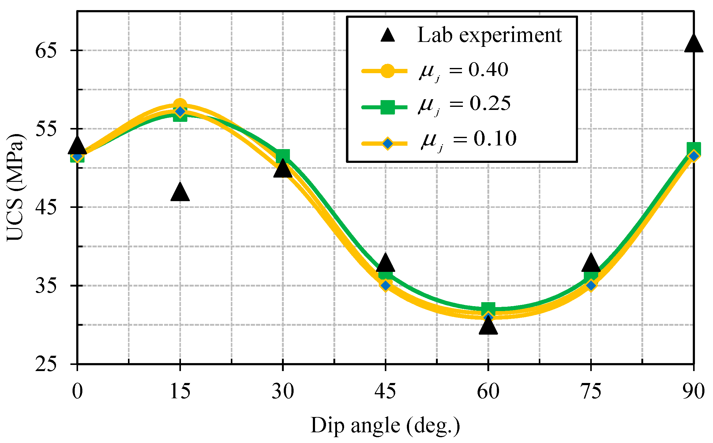
3.2.5. Joint Coefficient of Friction

The joint coefficient of friction began to work only after the joint bond broke to provide the residual shear strength. To learn about the effect of the interface residual shear strength on the failure behavior of transversely isotropic rock models, the joint coefficient of friction, ${\mu }_j$, was set to be 0.10, 0.25, and 0.40, whereas, the other joint parameters were kept constant, i.e., ${\overline{k}}_{nj}=0.5\times {10}^{13} \mathrm{N}/{\mathrm{m}}^3$, ${\overline{k}}_{sj}=1/3{\overline{k}}_{nj}$, ${\overline{\sigma }}_{cj}=23.8 \mathrm{MPa}$, $c_j=13.0 \mathrm{MPa}$, and ${\phi }_j=22.5°$. Figure 25 displays the UCS variation of transversely isotropic rock samples with different joint coefficients of friction. As shown in this figure, the joint coefficient of friction had a negligible influence on the resistance capability of transversely isotropic rock samples. For rock samples having low dip angles, e.g., α = 0° and 15°, the increment of the interface shear strength was not effective enough to affect UCS values because the rock samples tended to fail in the mode of tensile failure across interfaces. Furthermore, when the dip angle increased to be medium, such as α = 30°, 45°, 60°, and 75°, even though the shear strength of interfaces mattered, the joint coefficient of friction could not contribute to the peak stress of the whole rock model. This was due to the fact that the interface shear cracks began to occur quite close to the peak stress stage, as shown in Figure 12. Therefore, the joint coefficient of friction mainly contributed to the residual strength rather than to the UCS of the whole rock models, which agreed very well with Ref. [25]. For α = 90°, the transversely isotropic rock model failed according to tensile failure along interfaces, which accounted for the negligible influence of the joint coefficient of friction on UCS values.

3.2.6. Joint Tensile Strength

A parametric study on the influence of the joint tensile strength, ${\overline{\sigma }}_{cj}$, on the strength behavior of transversely isotropic rock models was carried out as well through varying this joint micro-mechanical parameter from 15.90 MPa to 31.80 MPa through 23.80 MPa while setting the other parameters constant. In accordance with Figure 26, the joint tensile strength had a slight influence on the UCS values of transversely isotropic rock models. For rock samples having low dip angles (α = 0°, 15°, and 30°), although the increment of the joint tensile strength somehow affected the strength behavior of transversely isotropic rock models, the influence was not significant. When the dip angle was medium, because the rock models failed in the mode of shear failure along interfaces, the increment of the interface tensile strength had a negligible influence on the strength of the whole rock models. Furthermore, although the rock model failed in the mode of tensile failure along interfaces, the UCS of the transversely isotropic rock sample was mainly contributed by the vertical intact materials. Thus, the change of joint tensile strength also had a negligible influence on the UCS value.

4. Conclusions

Particle flow modeling was undertaken to investigate the failure mechanism of transversely isotropic rocks under uniaxial compressive loading. After setting up a particle flow model with the PFC^3D software package according to the conceptual model proposed by Tien et al. [23], a parametric study was then carried out to investigate the effect of the interface dip angle and interface mechanical parameters on the failure mode and uniaxial compressive strength of the transversely isotropic rock models. The following conclusions can be drawn from the obtained particle flow modeling results:

(1)

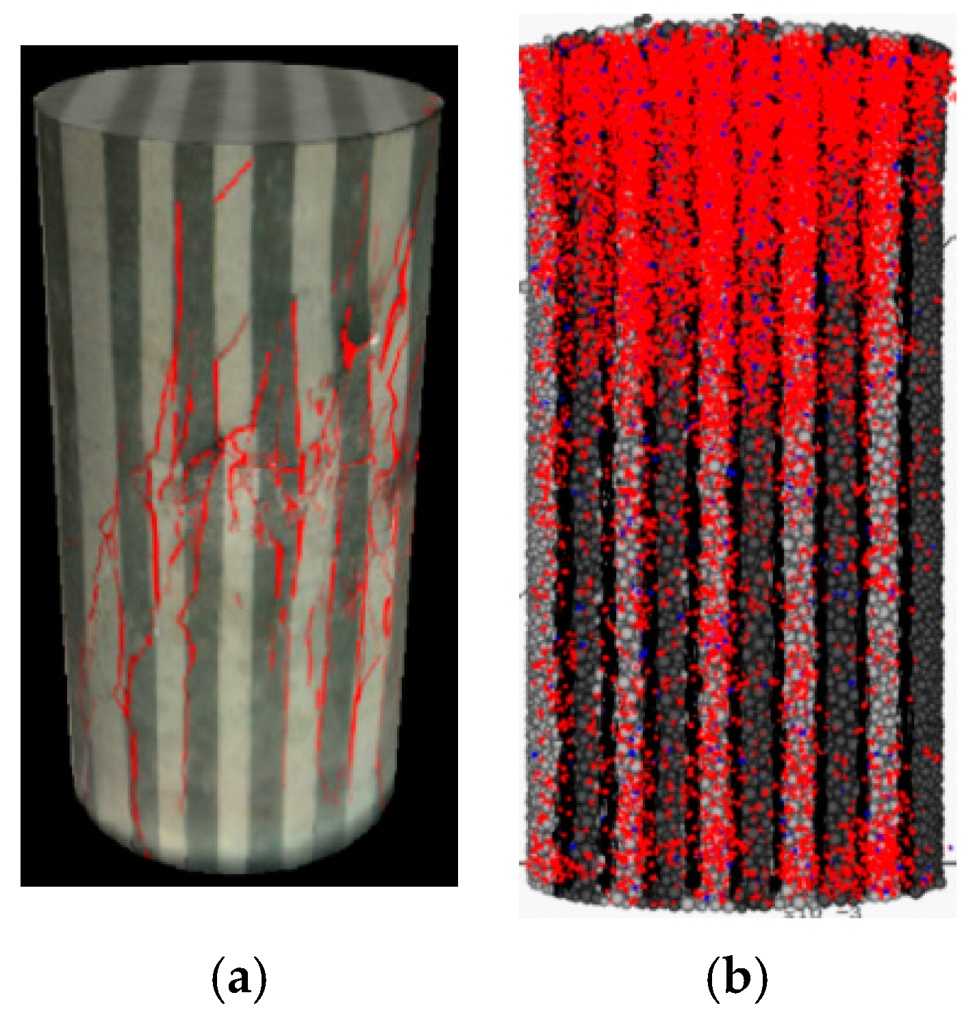
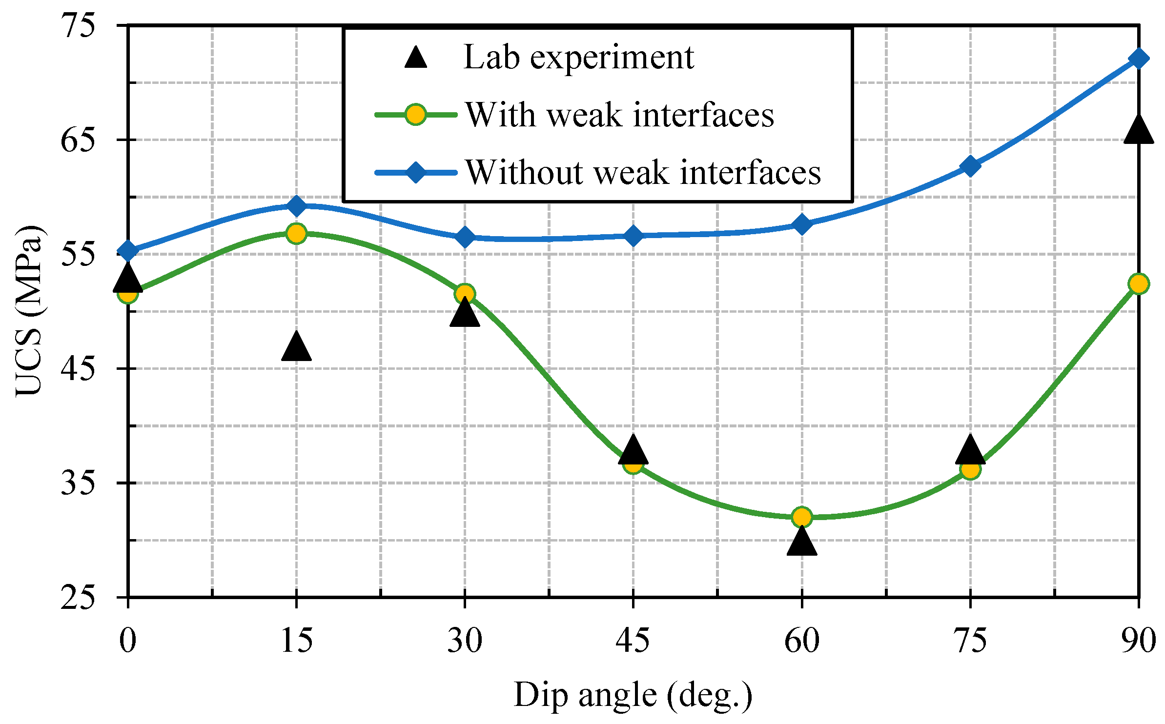
The interfaces interspaced in intact materials were pivotal elements to successfully build transversely isotropic rock models with a particle flow modeling method. With careful calibrations of the interface mechanical parameters, these simulated transversely isotropic rock models derived quite similar failure modes and UCS values to those obtained in physical experiments.

(2)

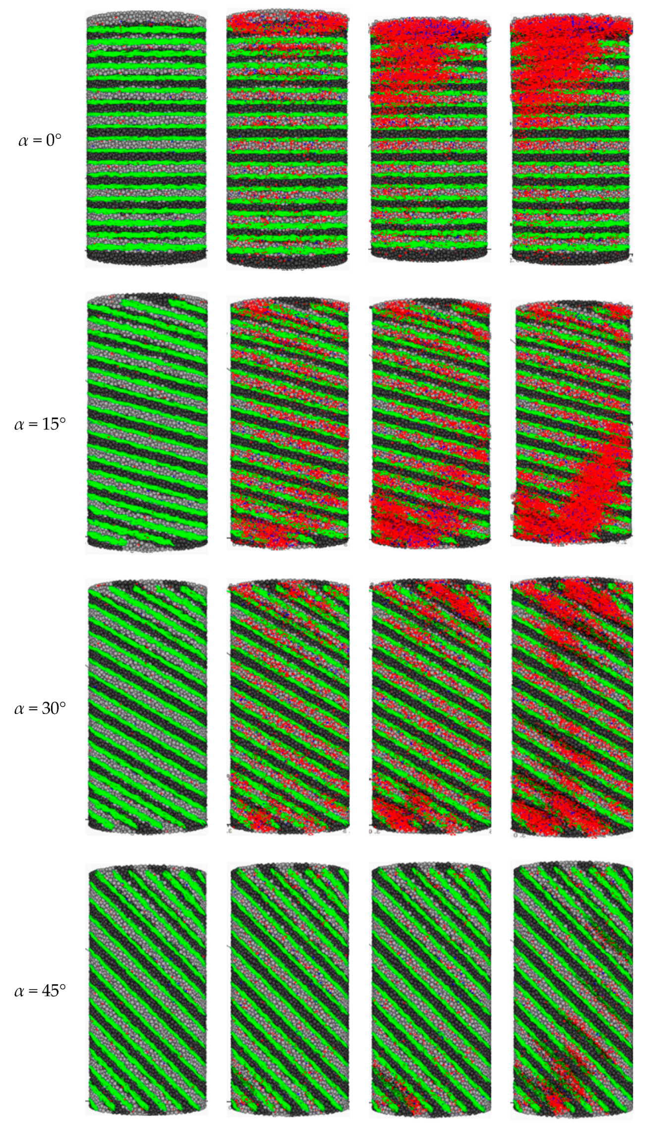
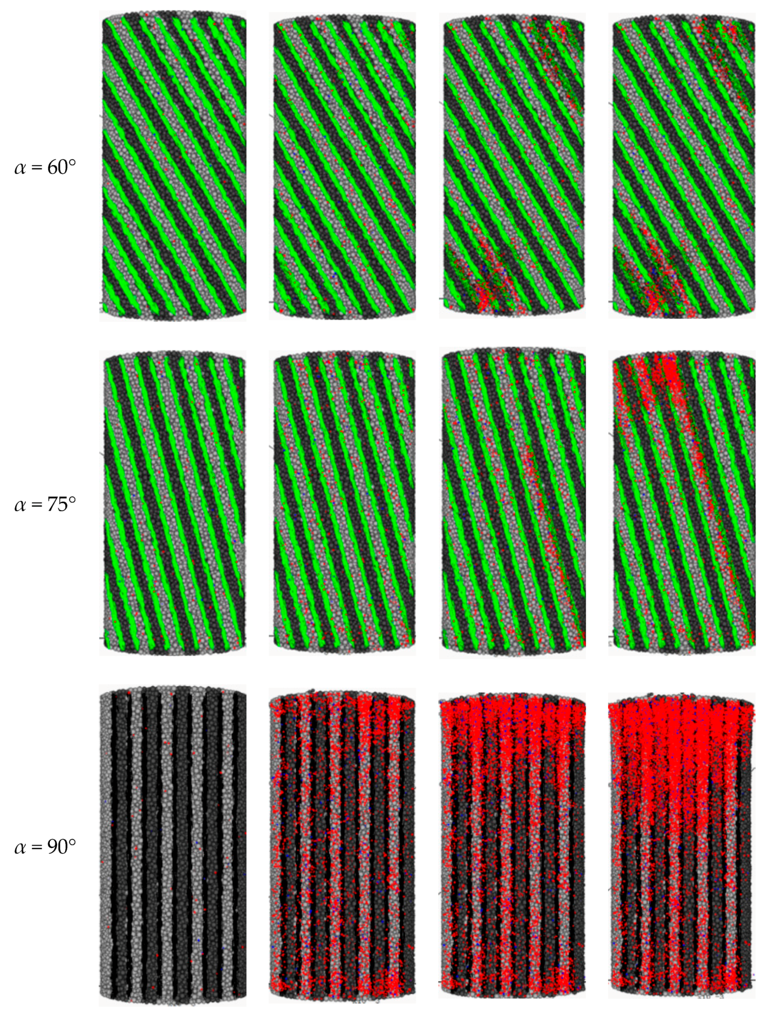
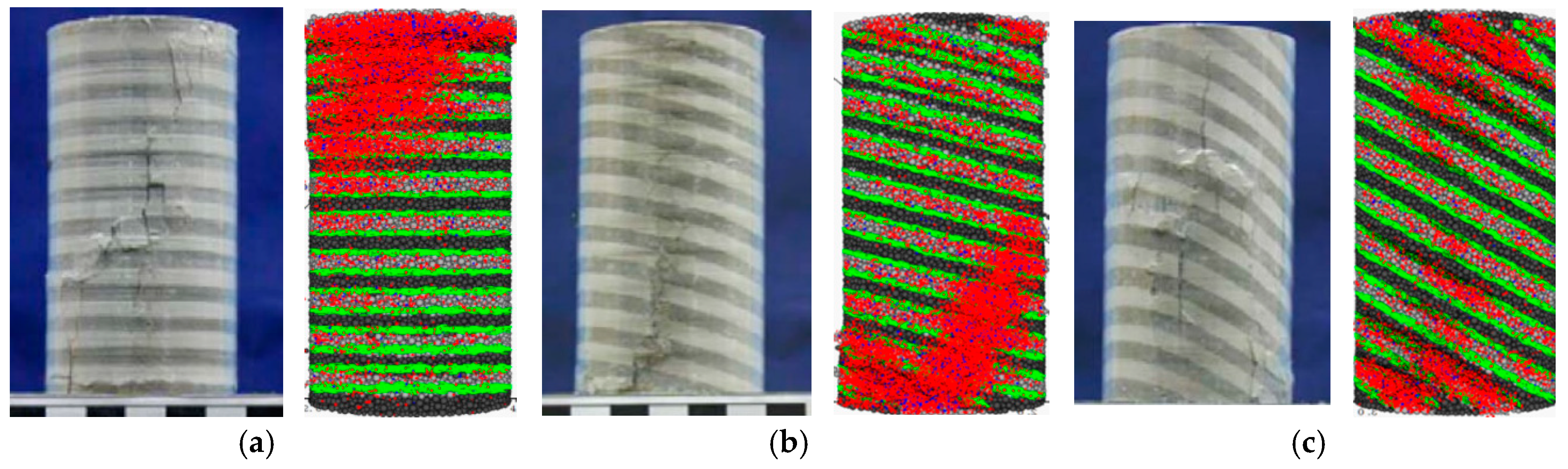
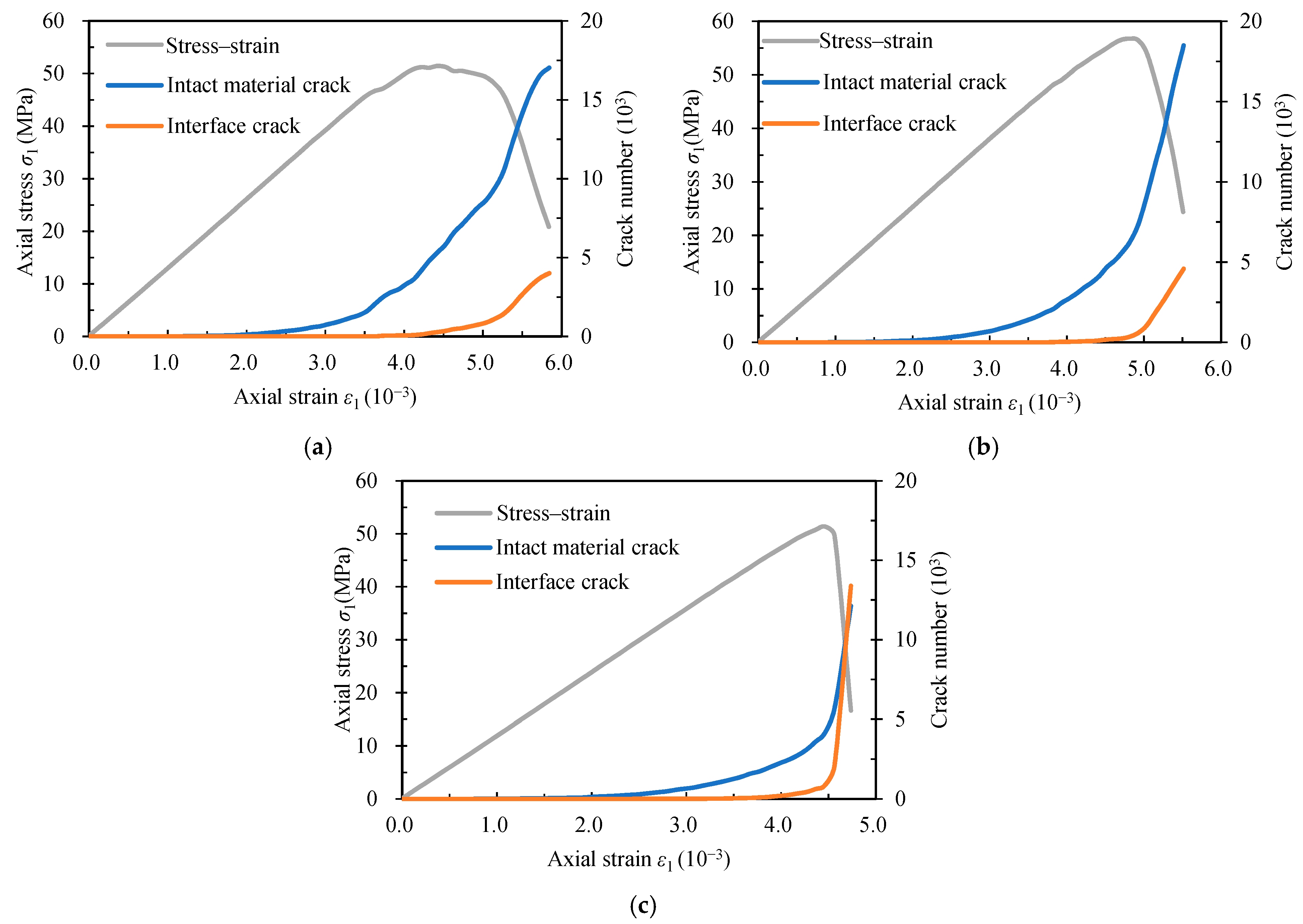
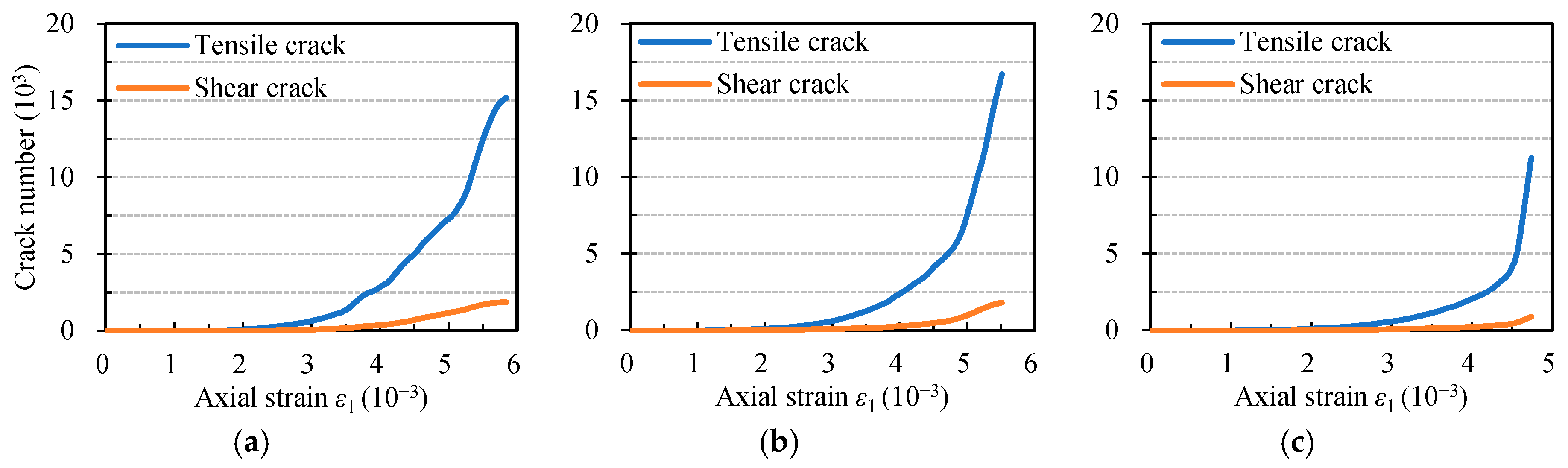
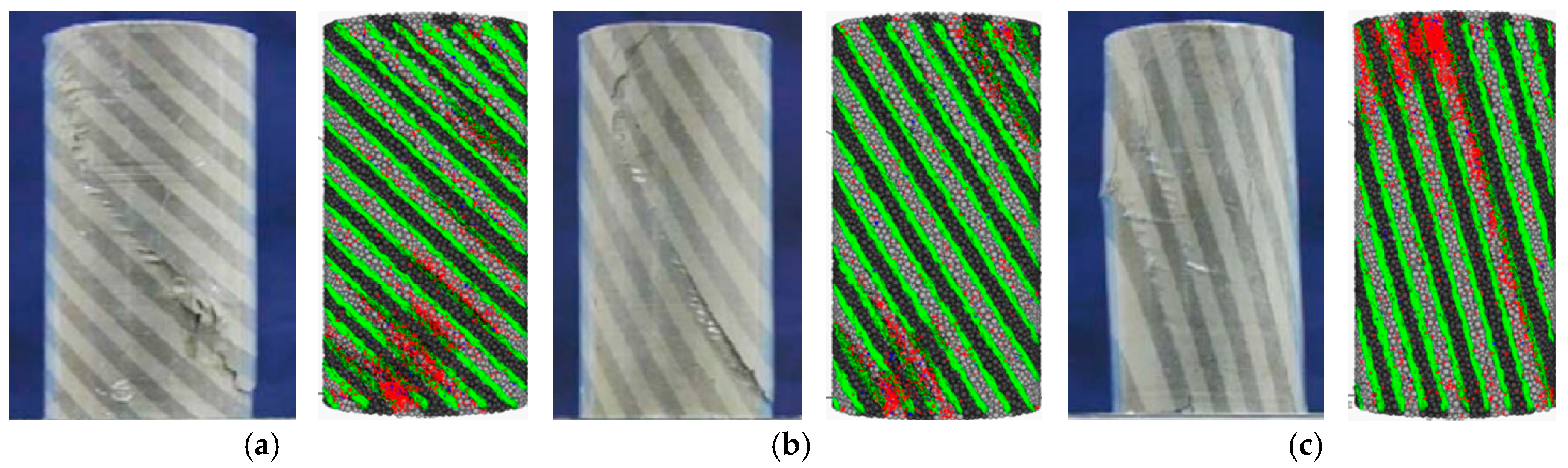
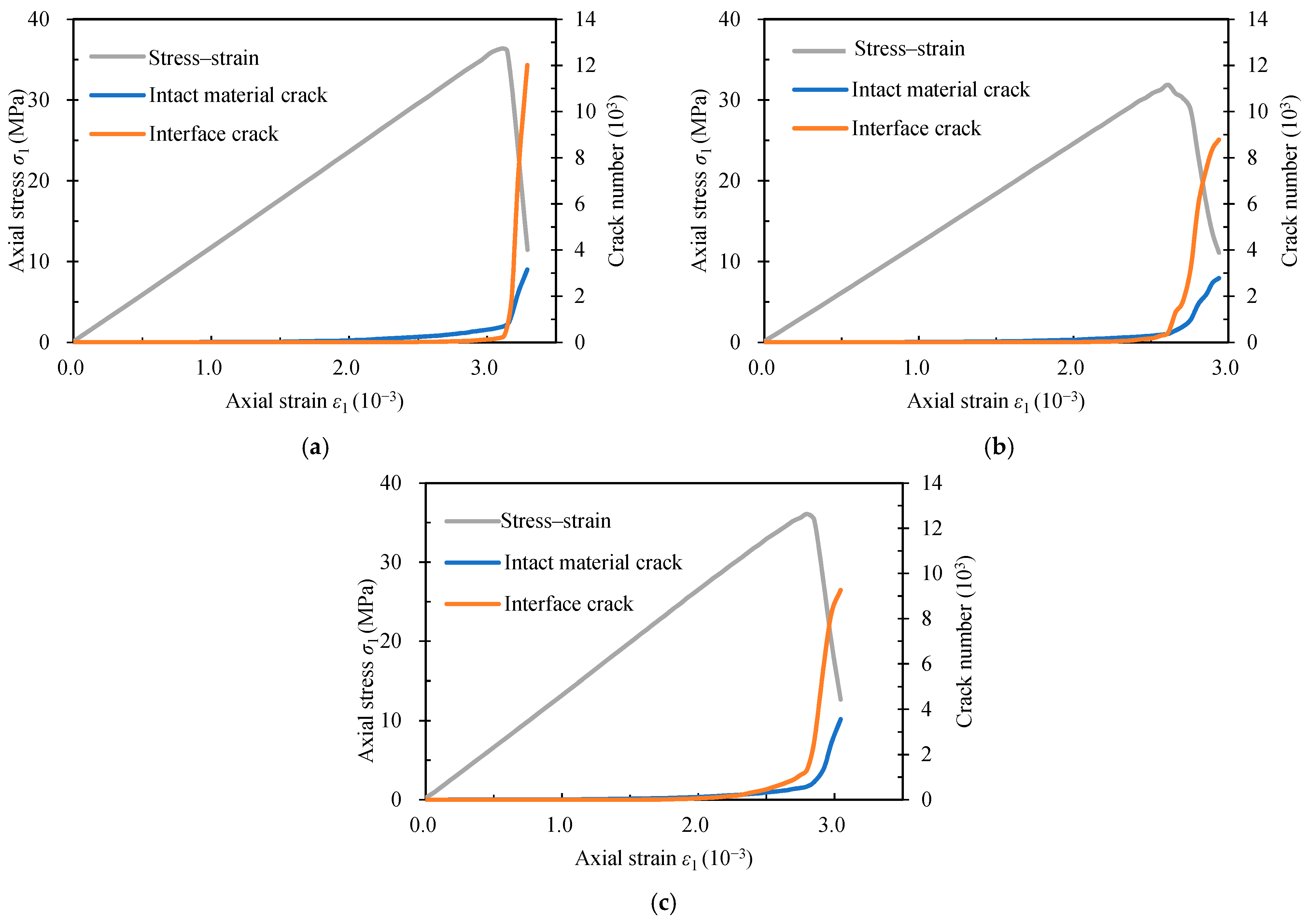
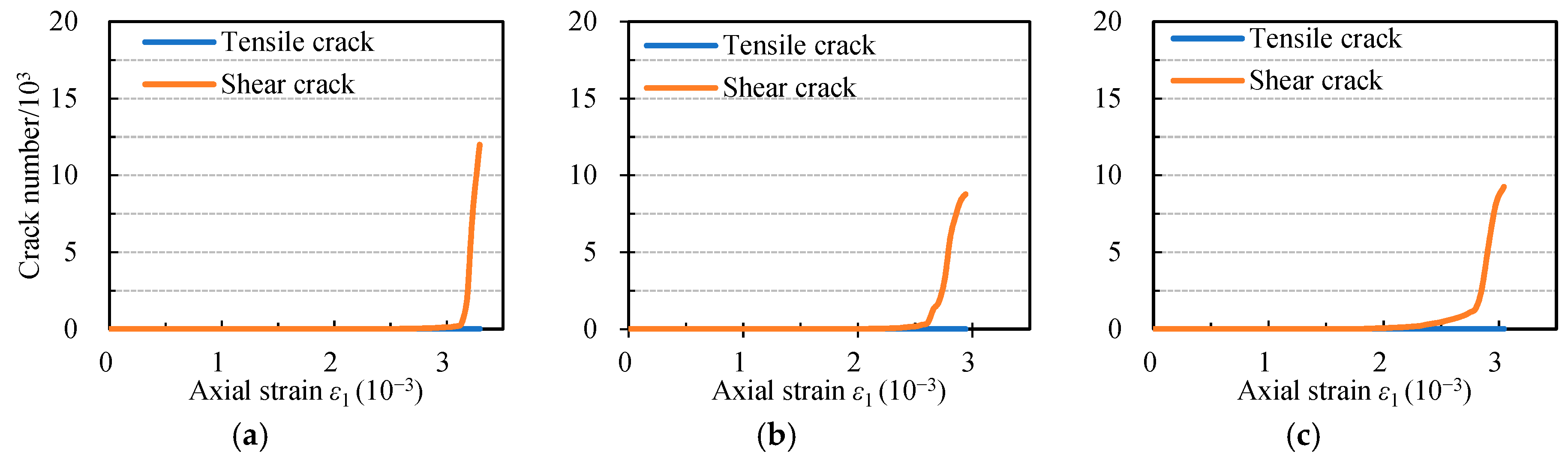
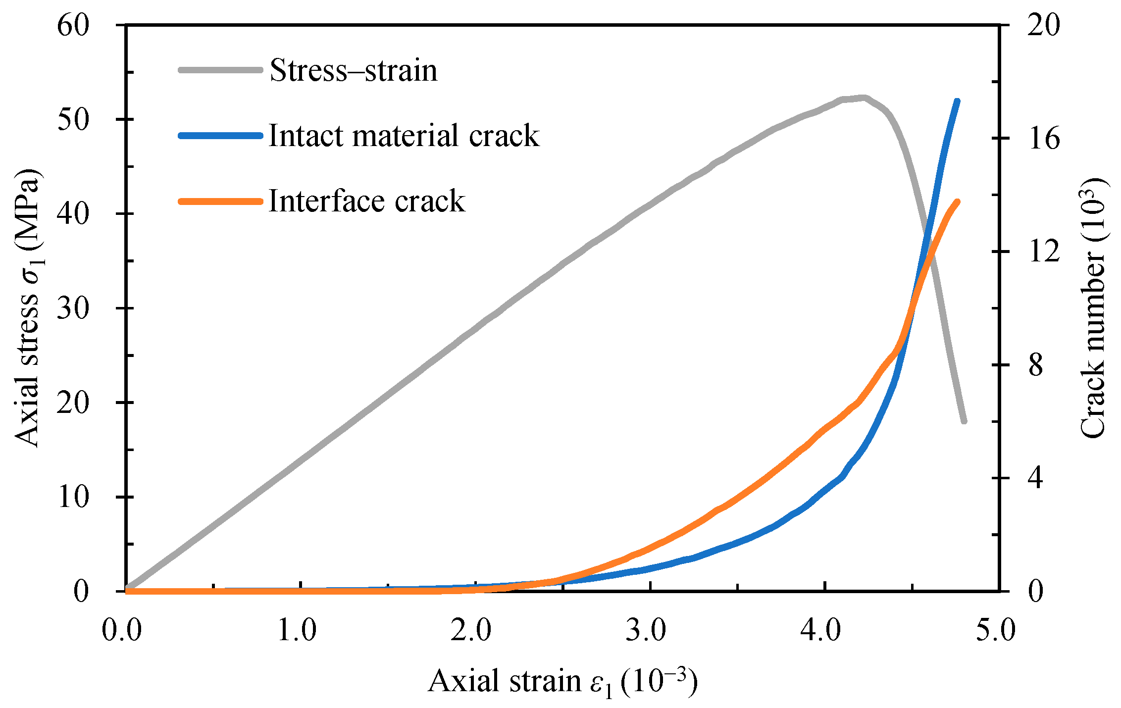
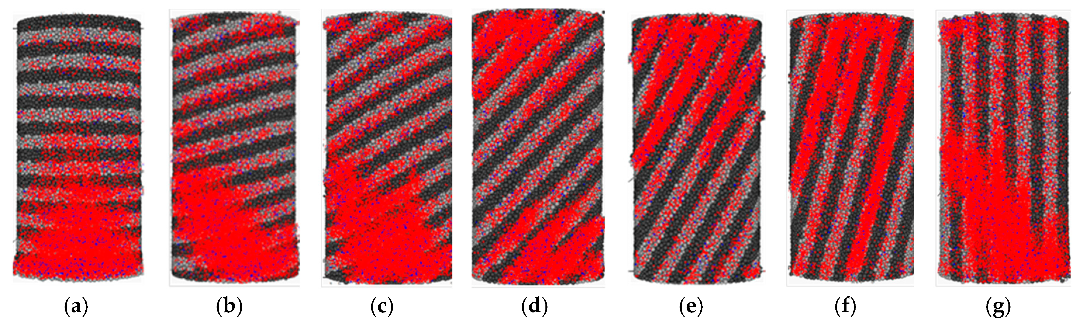
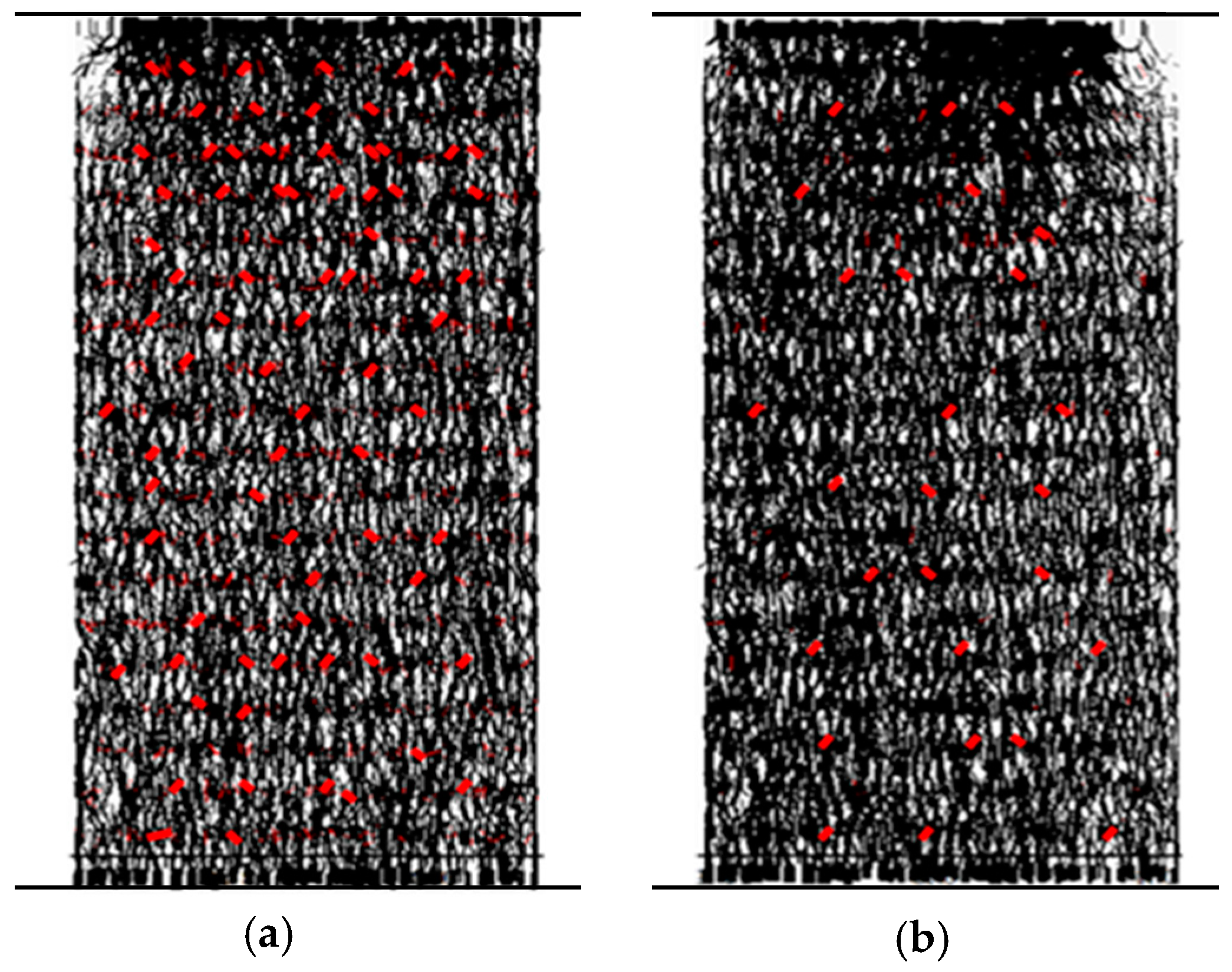
To highlight the effect of interfaces, the failure mode of transversely isotropic rock models was redefined according to the observed crack revolution at the meso level. Three basic failure modes were identified in the transversely isotropic rock models under uniaxial compressive loading: (a) tensile failure across interfaces, (b) shear failure along interfaces, and (c) tensile failure along interfaces.

(3)

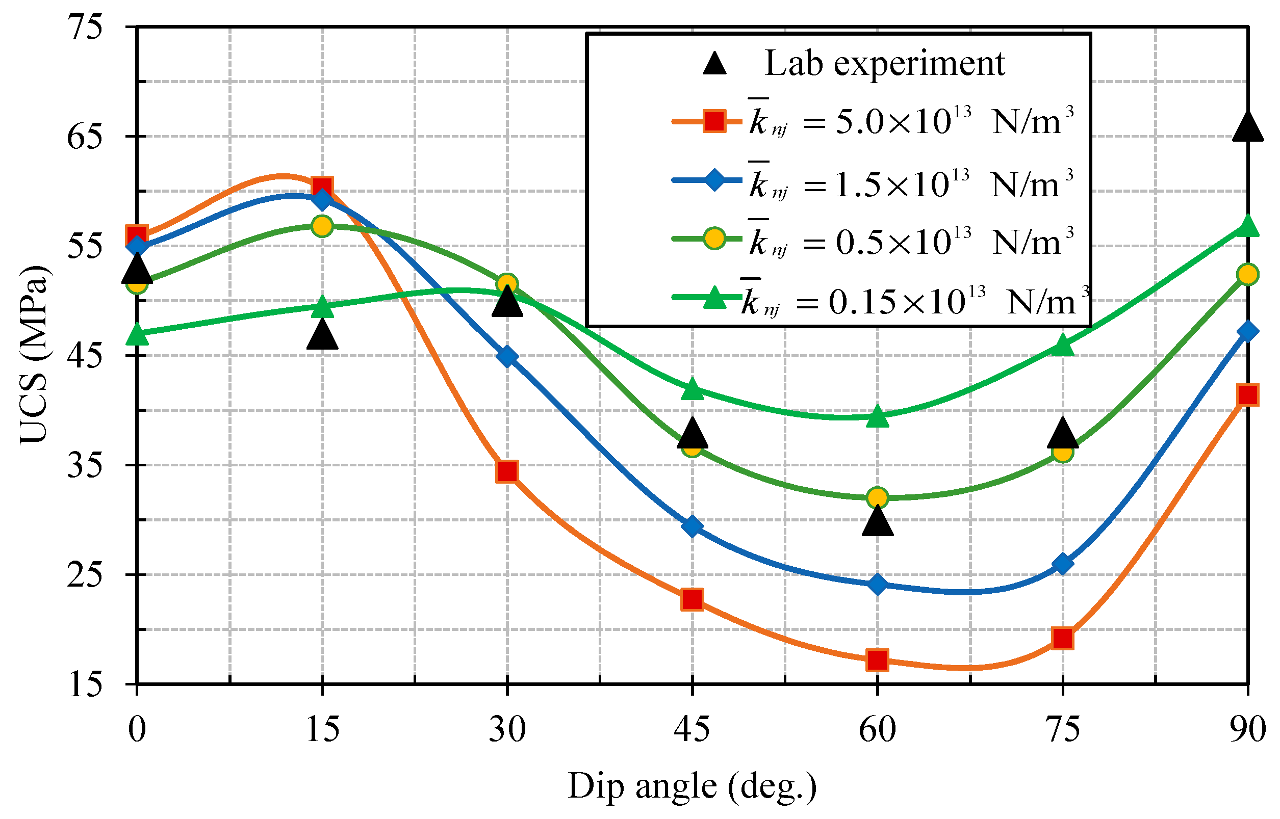
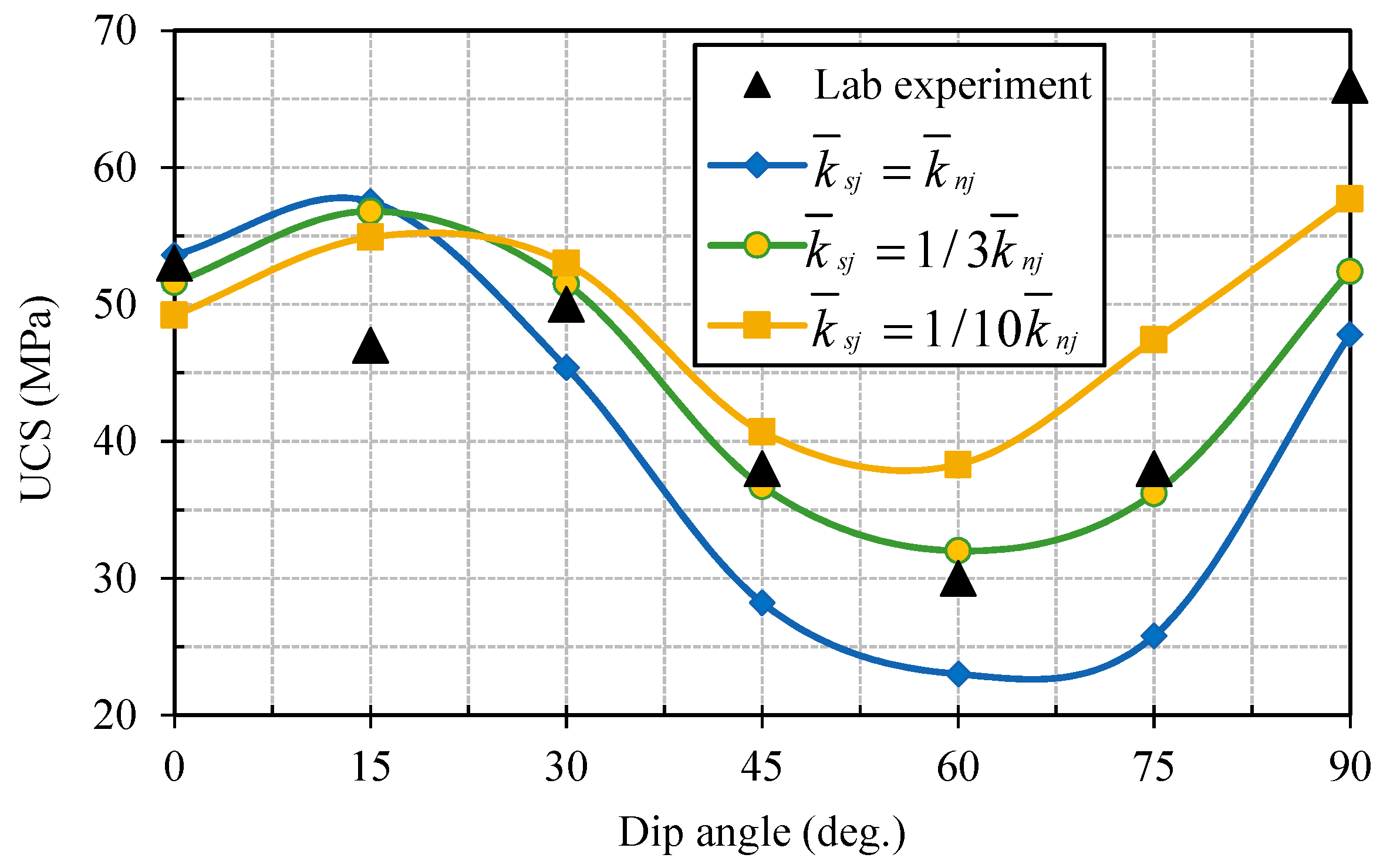
The joint normal stiffness and joint shear stiffness had a dramatic influence on the failure strength of transversely isotropic rock models. The difference of mechanical response to uniaxial compressive loading for each layered material accounted for the UCS variation with varying stiffness values.

(4)

The mechanical parameters for the bonded joint shear strength property had quite a different influence on the failure behavior of transversely isotropic rock models. The bonded joint cohesion and bonded joint friction angle, which contributed to the shear strength of interfaces, had a considerable influence on the UCS values, while the joint coefficient of friction, which contributed to the residual strength of interfaces, had a negligible influence on the UCS values.

(5)

The shear failure of interfaces was the dominant mechanism for anisotropic behavior of layered rock models, the change of joint tensile strength had a negligible influence on the UCS values of transversely isotropic rock models.

The present study put the emphasis on the failure mechanism of transversely isotropic rocks under the unconfined compression condition, whilst a further study on the anisotropic behavior of transversely isotropic rocks under the triaxial stress condition is undergoing. Moreover, the hydromechanical behavior of the transversely isotropic rocks is also a challenge topic that is of our interest. The following studies would provide useful guidelines for the stabilization control of engineering structures constructed in or on the transversely isotropic rocks.

References

1. Tan, X.; Konietzky, H.; Frühwirt, T.; Quoc Dan, D. Brazilian tests on transversely isotropic rocks: Laboratory testing and numerical simulations. Rock Mech. Rock Eng. 2015, 48, 1341–1351. [Google Scholar] [CrossRef]
2. Feng, X.T.; An, H. Hybrid intelligent method optimization of a soft rock replacement scheme for a large cavern excavated in alternate hard and soft rock strata. Int. J. Rock Mech. Min. Sci. 2004, 41, 655–667. [Google Scholar] [CrossRef]
3. Hudson, J.A.; Feng, X.T. Updated flowcharts for rock mechanics modelling and rock engineering design. Int. J. Rock Mech. Min. Sci. 2007, 44, 174–195. [Google Scholar] [CrossRef]
4. Okland, D.; Hydro, N.; Cook, J.M. Bedding-related borehole instability in high angle wells. In Proceedings of the EUROCK ‘98-Rock Mechanics in Petroleum Engineering, Trondheim, Norway, 8–10 July 1998. [Google Scholar]
5. Meier, T.; Rybacki, E.; Backers, T.; Dresen, G. Influence of bedding angle on borehole stability: A laboratory investigation of transversely isotropic oil shale. Rock Mech. Rock Eng. 2015, 48, 1535–1546. [Google Scholar] [CrossRef]
6. Zoback, M.D.; Barton, C.A.; Brudy, M.; Castillo, D.A.; Finkbeiner, T.; Grollimund, B.R.; Moos, D.B.; Peska, P.; Ward, C.D.; Wiprut, D.J. Determination of stress orientation and magnitude in deep wells. Int. J. Rock Mech. Min. Sci. 2003, 40, 1049–1076. [Google Scholar] [CrossRef]
7. Zhang, J. Borehole stability analysis accounting for anisotropies in drilling to weak bedding planes. Int. J. Rock Mech. Min. Sci. 2013, 60, 160–170. [Google Scholar] [CrossRef]
8. Liu, R.C.; Li, B.; Jiang, Y.J. Critical hydraulic gradient for nonlinear flow through rock fracture networks: The roles of aperture, surface roughness, and number of intersections. Adv. Water Res. 2016, 88, 53–65. [Google Scholar] [CrossRef]
9. Zhou, Y.Y.; Feng, X.T.; Xu, D.P.; Fan, Q.X. Experimental investigation of the mechanical behavior of bedded rocks and its implication for high sidewall caverns. Rock Mech. Rock Eng. 2016, 49, 3643–3669. [Google Scholar] [CrossRef]
10. Cai, M.; Kaiser, P.K.; Tasaka, Y.; Minami, M. Determination of residual strength parameters of jointed rock masses using the GSI system. Int. J. Rock Mech. Min. Sci. 2007, 44, 247–265. [Google Scholar] [CrossRef]
11. Gatelier, N.; Pellet, F.; Loret, B. Mechanical damage of an anisotropic porous rock in cyclic triaxial tests. Int. J. Rock Mech. Min. Sci. 2002, 39, 335–354. [Google Scholar] [CrossRef]
12. Kim, K.Y.; Zhuang, L.; Yang, H.; Kim, H.; Min, K.B. Strength anisotropy of Berea sandstone: Results of X-ray computed tomography, compression tests, and discrete modeling. Rock Mech. Rock Eng. 2016, 49, 1201–1220. [Google Scholar] [CrossRef]
13. Heng, S.; Guo, Y.T.; Yang, C.H.; Daemen, J.K.; Li, Z. Experimental and theoretical study of the anisotropic properties of shale. Int. J. Rock Mech. Min. Sci. 2015, 74, 58–68. [Google Scholar] [CrossRef]
14. Kulatilake, P.H.S.W.; He, W.; Um, J.; Wang, H. A physical model study of jointed rock mass strength under uniaxial compressive loading. Int. J. Rock Mech. Min. Sci. 1997, 34, 165.e1–165.e15. [Google Scholar] [CrossRef]
15. Yang, Z.Y.; Chen, J.M.; Huang, T.H. Effect of joint sets on the strength and deformation of rock mass models. Int. J. Rock Mech. Min. Sci. 1998, 35, 75–84. [Google Scholar] [CrossRef]
16. Yang, X.X.; Jing, H.W.; Tang, C.A.; Yang, S.Q. Effect of parallel joint interaction on mechanical behavior of jointed rock mass models. Int. J. Rock Mech. Min. Sci. 2017, 92, 40–53. [Google Scholar] [CrossRef]
17. Bahaaddini, M.; Sharrock, G.; Hebblewhite, B.K.; Mitra, R. Direct shear tests to model the shear behavior of rock joints by PFC2D. In Proceedings of the 46th US Rock Mechanics/Geomechanics Symposium, American Rock Mechanics Association, Chicago, IL, USA, 24–27 June 2012. [Google Scholar]
18. Bahaaddini, M.; Sharrock, G.; Hebblewhite, B.K. Numerical investigation of the effect of joint geometrical parameters on the mechanical properties of a non-persistent jointed rock mass under uniaxial compression. Comput. Geotech. 2013, 49, 206–225. [Google Scholar] [CrossRef]
19. Chiu, C.C.; Wang, T.T.; Weng, M.C.; Huang, T.H. Modeling the anisotropic behavior of jointed rock mass using a modified smooth-joint model. Int. J. Rock Mech. Min. Sci. 2013, 62, 14–22. [Google Scholar] [CrossRef]
20. Prudencio, M.; Van Sint Jan, M. Strength and failure modes of rock mass models with non-persistent joints. Int. J. Rock Mech. Min. Sci. 2007, 44, 890–902. [Google Scholar] [CrossRef]
21. Park, B.; Min, K.B. Bonded-particle discrete element modeling of mechanical behavior of transversely isotropic rock. Int. J. Rock Mech. Min. Sci. 2015, 76, 243–255. [Google Scholar] [CrossRef]
22. Yang, S.Q.; Huang, Y.H. Particle flow study on strength and meso-mechanism of Brazilian splitting test for jointed rock mass. Acta Mech. Sin. 2014, 30, 547–558. [Google Scholar] [CrossRef]
23. Tien, Y.M.; Kuo, M.C.; Juang, C.H. An experimental investigation of the failure mechanism of simulated transversely isotropic rocks. Int. J. Rock Mech. Min. Sci. 2006, 43, 1163–1181. [Google Scholar] [CrossRef]
24. Potyondy, D.O.; Cundall, P.A. A bonded-particle model for rock. Int. J. Rock Mech. Min. Sci. 2004, 41, 1329–1364. [Google Scholar] [CrossRef]
25. Itasca Consulting Group Inc. PFC3D-Particle Flow Code in Three Dimensions, version 4.0; Itasca Consulting Group Inc.: Minneapolis, MN, USA, 2008. [Google Scholar]
26. Mas Ivars, D.M.; Pierce, M.E.; Darcel, C.; Juan, R.M.; Potyondy, D.O.; Young, R.P.; Cundall, P.A. The synthetic rock mass approach for jointed rock mass modelling. Int. J. Rock Mech. Min. Sci. 2011, 48, 219–244. [Google Scholar] [CrossRef]
27. Kulatilake, P.H.S.W.; Malama, B.; Wang, J.L. Physical and particle flow modeling of jointed rock block behavior under uniaxial loading. Int. J. Rock Mech. Min. Sci. 2001, 38, 641–657. [Google Scholar] [CrossRef]
28. Yang, X.X.; Kulatilake, P.H.S.W.; Jing, H.W.; Yang, S.Q. Numerical simulation of a jointed rock block mechanical behavior adjacent to an underground excavation and comparison with physical model test results. Tunn. Undergr. Space Technol. 2015, 50, 129–142. [Google Scholar] [CrossRef]
29. Yang, X.X.; Kulatilake, P.H.S.W.; Chen, X.; Jing, H.W.; Yang, S.Q. Particle flow modeling of rock blocks with nonpersistent open joints under uniaxial compression. Int. J. Geomech. 2016, 16, 04016020-1-17. [Google Scholar] [CrossRef]
30. Yang, X.X.; Qiao, W.G. Numerical investigation of the shear behavior of granite materials containing discontinuous joints by utilizing the flat-joint model. Comput. Geotech. 2018, 104, 69–80. [Google Scholar] [CrossRef]
31. Tien, Y.M.; Kuo, M.C. A failure criterion for transversely isotropic rocks. Int. J. Rock Mech. Min. Sci. 2001, 38, 399–412. [Google Scholar] [CrossRef]
32. Yasar. Failure and failure theories for anisotropic rocks. In Proceedings of the 17th International Mining Congress and Exhibition of Turkey (IMCET), Ankara, Turkey, 19–22 June 2001; pp. 417–424. [Google Scholar]
33. Autio, J.; Wanne, T.; Potyondy, D. Particle mechanical simulation of the effect of schistosity on strength and deformation of hard rock. In Proceedings of the 5th North American Rock Mechanics Symposium & 17th Tunneling Association of Canada Conference: NARMS-TAC, Toronto, ON, Canada, 7–10 July 2002; Vo1ume 1, pp. 275–282. [Google Scholar]
34. Nasseri, M.H.B.; Rao, K.S.; Ramamurthy, T. Anisotropic strength and deformation behavior of Himalayan schists. Int. J. Rock Mech. Min. Sci. 2002, 40, 3–23. [Google Scholar] [CrossRef]
35. Cho, J.W.; Kim, H.; Jeon, S.; Min, K.B. Deformation and strength anisotropy of Asan gneiss, Boryeong shale, and Yeoncheon schist. Int. J. Rock Mech. Min. Sci. 2012, 50, 158–169. [Google Scholar] [CrossRef]
36. Fjaer, E.; Nes, O.M. Strength anisotropy of Mancos shale. In Proceedings of the 47th US Rock Mechanics/Geomechanics Symposium, San Francisco, CA, USA, 23–26 June 2013. [Google Scholar]
Figure 1. A typical transversely isotropic rock sample (α = 0°).
Processes 06 00171 g001
Figure 2. The contact model and parallel bond model: (a) intact material, (b) particle contact, and (c) parallel bond.
Processes 06 00171 g002
Figure 3. Numerically developed transversely isotropic rock samples having different interface dip angles: (a) α = 0°, (b) α = 15°, (c) α = 30°, (d) α = 45°, (e) α = 60°, (f) α = 75°, and (g) α = 90°.
Processes 06 00171 g003
Figure 4. Smooth joint model: (a) numerical analog, and (b) physical analog.
Processes 06 00171 g004
Figure 5. Constitutive law for a bonded smooth joint model: (a) normal force, F n j , versus normal displacement, U n j ; (b) shear force, F s j , versus shear displacement, U s j ; and (c) strength envelope.
Processes 06 00171 g005
Figure 6. Calibration process for determination of smooth joint parameters.
Processes 06 00171 g006
Figure 7. Failure process of transversely isotropic jointed rock models.
Processes 06 00171 g007aProcesses 06 00171 g007b
Figure 8. Failure modes of transversely isotropic jointed rock models having dip angles of (a) α = 0°, (b) α = 15°, and (c) α = 30°. (Note that the failure images of physical samples were adopted from Ref. [23]).
Processes 06 00171 g008
Figure 9. Crack number evolution of transversely isotropic rock models with dip angles of (a) α = 0°, (b) α = 15°, and (c) α = 30°.
Processes 06 00171 g009
Figure 10. Intact material crack number evolution of transversely isotropic jointed rock models having dip angles of (a) α = 0°, (b) α = 15° and (c) α = 30°.
Processes 06 00171 g010
Figure 11. Failure modes of transversely isotropic jointed rock models having dip angles of (a) α = 45°, (b) α = 60°, and (c) α = 75°. (Note that the failure images of physical samples were adopted from Ref. [23]).
Processes 06 00171 g011
Figure 12. Crack number evolution of transversely isotropic rock models with dip angles of (a) α = 45°, (b) α = 60° and (c) α = 75°.
Processes 06 00171 g012
Figure 13. Intact material crack number evolution of transversely isotropic jointed rock models having dip angles of (a) α = 45°, (b) α = 60° and (c) α = 75°.
Processes 06 00171 g013
Figure 14. Failure modes of transversely isotropic jointed rock model having dip angle of 90°: (a) experiment sample, and (b) numerical sample. (Note that the failure images of physical samples were adopted from Ref. [23]).
Processes 06 00171 g014
Figure 15. Evolution of crack number in transversely isotropic jointed rock models having dip angle of 90°.
Processes 06 00171 g015
Figure 16. Failure modes of transversely isotropic rocks without weak interfaces: (a) α = 0°, (b) α = 15°, (c) α = 30°, (d) α = 45°, (e) α = 60°, (f) α = 75°, and (g) α = 90°.
Processes 06 00171 g016
Figure 17. Comparison of UCS of transversely isotropic rocks with and without weak interfaces.
Processes 06 00171 g017
Figure 18. UCS variation of transversely isotropic rock samples with different joint normal stiffness.
Processes 06 00171 g018
Figure 19. UCS variation of transversely isotropic rock samples with different joint shear stiffness.
Processes 06 00171 g019
Figure 20. Force chains in the transversely isotropic rock models having horizontal interfaces with different joint normal stiffness at peak stress: (a) k ¯ n j = 0.15 × 10 13   N / m 3 , and (b) k ¯ n j = 5.0 × 10 13   N / m 3 . Note that the black chain and red chain imply compression force and tension force, respectively, and the force quantity is proportional to the chain thickness.
Processes 06 00171 g020
Figure 21. Strength variation of transversely isotropic rock samples with different bonded joint cohesion.
Processes 06 00171 g021
Figure 22. Interface shear crack proportion variation with different bonded joint cohesion.
Processes 06 00171 g022
Figure 23. Strength variation of transversely isotropic rock samples with bonded joint friction angle.
Processes 06 00171 g023
Figure 24. Interface shear crack proportion variation with different bonded joint friction angle.
Processes 06 00171 g024
Figure 25. Strength variation of transversely isotropic rock samples with different joint coefficient of friction.
Processes 06 00171 g025
Figure 26. Strength variation of transversely isotropic rock samples with different joint tensile strength.
Processes 06 00171 g026