Novel Triplet Loss-Based Domain Generalization Network for Bearing Fault Diagnosis with Unseen Load Condition

Abstract

In the real industrial manufacturing process, due to the constantly changing operational loads of equipment, it is difficult to collect data from all load conditions as the source domain signal for fault diagnosis. Therefore, the appearance of unseen load vibration signals in the target domain presents a challenge and research hotspot in fault diagnosis. This paper proposes a triplet loss-based domain generalization network (TL-DGN) and then applies it to an unseen domain bearing fault diagnosis. TL-DGN first utilizes a feature extractor to construct a multi-source domain classification loss. Furthermore, it measures the distance between class data from different domains using triplet loss. The introduced triplet loss can narrow the distance between samples of the same class in the feature space and widen the distance between samples of different classes based on the action of the cross-entropy loss function. It can reduce the dependency of the classification boundary on bearing operational loads, resulting in a more generalized classification model. Finally, two comparative experiments with fault diagnosis models without triplet loss and other classification models demonstrate that the proposed model achieves superior fault diagnosis performance.

1. Introduction

In the discrete industry, large-scale equipment is typically a complex system with numerous components. Among them, rotating machinery such as fans and pumps have been widely utilized, yet prolonged operation in harsh environments may lead to wear and subsequent failures. Such failures not only disturb the normal operation of the equipment, but also have security risks. Hence, research on fault diagnosis of rotating machinery holds significant importance in quickly identifying fault locations and severity, which can ensure the safe and smooth operation of equipment and provides manufacturing enterprises with clear and prompt demands. During the operation of rotating machinery, vibration signals containing information about the equipment’s operating status are generated. When equipment malfunctions, changes in the operating status result in vibration signals differing from those during normal operation. Intelligent sensing units such as sensors can collect vibration signals from various parts of the rotating machinery, which can be utilized for process monitoring and fault diagnosis [1]. Moreover, with the development of data-driven fault diagnosis methods, research based on vibration signals has become a hotspot. Data-driven methods can make full use of operational data obtained from monitored equipment to diagnose faults through data acquisition, feature extraction, and modeling [2].

There are three main data-driven methods used in the fault diagnosis of rotating machinery: signal processing-based methods, machine learning-based methods, and deep learning-based methods. Signal processing-based fault diagnosis involves processing vibration data using time-frequency analysis techniques to extract signals that reflect faults [3]. These methods include adaptive mode decomposition [4], short-time Fourier transform [5], wavelet transform [6,7], etc. However, such methods require prior information about fault characteristic frequencies, which limits their applicability. Later, machine learning methods have been widely combined with signal processing methods to improve model classification performance. For example, some studies decompose vibration signals of roller bearing faults into a finite number of stationary intrinsic mode functions and extract energy features as input vectors for artificial neural networks [8]. Chen et al. proposed a multi-fault diagnosis model based on wavelet-PCA and fuzzy K-nearest neighbor (KNN) for rolling bearing data [9]. Wang et al. developed a rolling bearing fault diagnosis model based on wavelet packet denoising and random forests [10].

Nowadays, due to the increasingly complex structure of rotating machinery and the variations in vibration signals due to changes in operating conditions, manually extracting features for diagnosis is time consuming. Thus, a key challenge in rotating equipment fault diagnosis is to develop more efficient autonomous feature extraction and diagnostic methods that can effectively identify faults under variable loads and enhance the generalization of diagnostic models. Therefore, deep learning methods have been widely introduced into fault diagnosis modeling due to their excellent learning performance. Deep learning methods can establish end-to-end models for vibration signals, autonomously extract features, and identify healthy states [11]. Deep models such as deep belief networks [7], stacked autoencoders [12], and convolutional neural networks [13] are widely applied in rolling bearing fault diagnosis [14]. Wang et al. proposed a multi-scale learning neural network containing one-dimensional and two-dimensional convolution channels [15], capable of learning the local correlations of periodic signals such as neighboring and non-neighboring intervals in vibration data. Niu et al. proposed an adaptive deep belief network-based fault diagnosis method for rolling bearings using principal component analysis and parameter-corrected linear unit activation layers [16]. Cui et al. proposed a feature distance stack autoencoder for rolling bearing fault diagnosis [17], first classifying normal and faulty data using a simple linear support vector machine, then classifying faults using the proposed feature distance stack autoencoder. Nie et al. proposed a normalized recursive neural network for noisy label fault diagnosis, utilizing normalized long short-term memory to improve training and introducing forward cross-entropy loss to address the negative effects of noisy labels [18]. Wang et al. proposed an imbalanced fault diagnosis method based on a conditional variational autoencoder generative adversarial network [19], initially using the encoder network of the conditional variational autoencoder to obtain the distribution of fault samples, then generating a large number of similar fault samples through the encoder network, and finally continuously optimizing the parameters of the generator, discriminator, and classifier through adversarial learning mechanisms, applying the trained model for intelligent fault diagnosis of planetary gearboxes.

However, most existing fault detection methods are designed for situations where the target domain is visible, meaning the target domain participates in model training. In real industrial manufacturing environments, target domain data may not be available for training. On the one hand, the operational loads of equipment vary greatly, making it impossible to collect complete fault signals for every load condition. On the other hand, suppose a fault occurs the first time the equipment operates under a certain load. In that case, there are no fault signals collected for that load condition at that time. Additionally, some equipment may not be allowed to operate in a faulty state for an extended period, making it impossible to collect complete fault data. In such cases, how to extract universal and effective information from available source domain data and apply it to fault diagnosis in unseen domains is crucial for intelligent diagnostic technologies. In recent years, in response to the issue of fault diagnosis in unseen domain bearings, an increasing number of researchers have proposed fault diagnosis algorithms based on domain generalization networks [20]. The main idea of domain generalization is to learn from one or multiple source domains and then extract a domain-agnostic model that can be applied to an unseen domain [21,22]. Chen et al. proposed a generic domain-regressive fault diagnosis model for unseen bearing faults [23]. Shi et al. developed a domain transferability-based deep domain generalization model for rotary machinery cross-domain fault diagnosis [24]. Zhao and Shen designed a federated domain generalization framework combining edge computing and cloud computing to realize robust fault diagnosis [25]. Fan et al. developed a deep mixed domain generalization network to achieve cross-domain fault diagnosis under unseen working conditions or machines [26]. Wang and Liu proposed a triplet loss-guided adversarial domain adaptation method [27]. The paper of [27] addressed the domain shift issue by concatenating two mini-batches of data from the source and target domains into a single mini-batch and incorporating triplet loss. The commonality between our paper and [27] lies in the use of triplet loss to minimize the distribution difference between classes in the feature space. The difference between domain adaptation and domain generalization is shown in Figure 1 and Figure 2. In Figure 1, the model focuses on whether the distribution between the source and target domains can be aligned in a certain space so that the model can classify the target domain correctly but ignores the effect of the model in other unseen domains. In Figure 2, domain generalization is to learn a classification model that can be applied to unseen domains through multiple source domains and pay more attention to the generalization ability of the model.

This paper introduces the triplet loss-based domain generalization network (TL-DGN) method for diagnosing faults in unseen domain bearings, addressing challenges from differences in load conditions between training and testing samples. By integrating the triplet loss, it effectively tackles this issue. The TL-DGN method uses both cross-entropy loss for classification accuracy and triplet loss to manage feature distribution, promoting proximity among similar samples and separation among dissimilar ones. This results in a more generalized classification boundary. The TL-DGN method demonstrates discrimination between fault categories, achieves low classification errors through cross-entropy loss, facilitates feature clustering, and enhances generalization capabilities, making it less sensitive to changes in load conditions. The TL-DGN method proposed in this paper can integrate information from multiple source domains based on triplet loss. This method can delineate nonlinear boundaries among data categories from these domains, thus generalizing to unseen domains for fault classification.

The remainder of this paper is organized as follows. In Section 2, a brief introduction of domain generalization is given. In Section 3, the detailed description of triplet loss is shown. In Section 4, the structure of TL-DGN and the flowchart of the TL-DGN method are given. Section 5 validates the effectiveness of the proposed algorithm through a bearing data set and a gearbox data set.

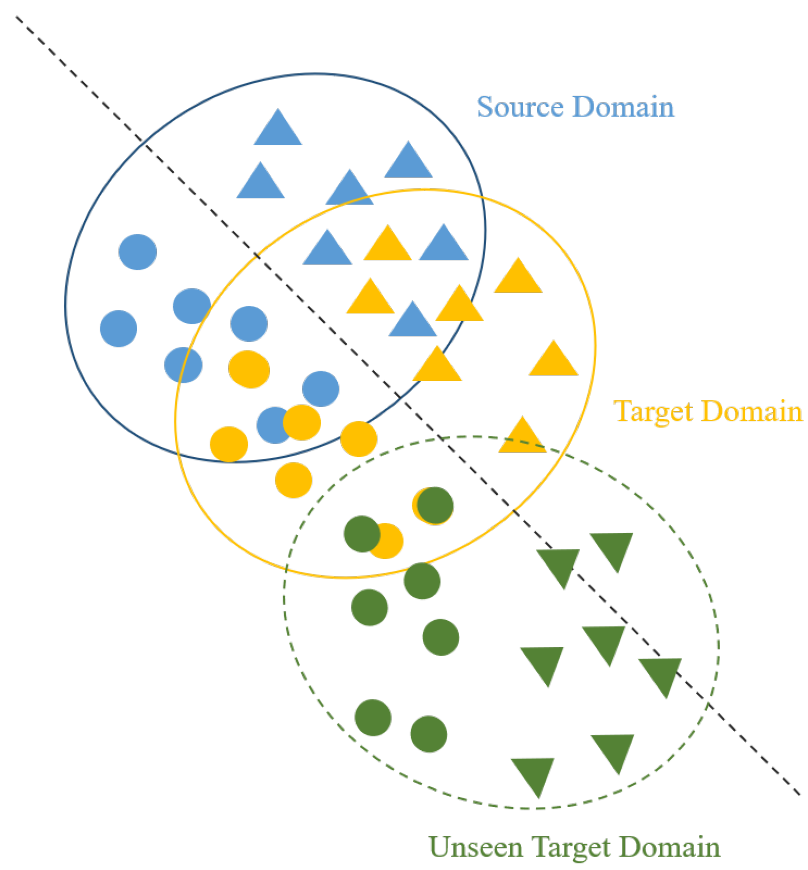
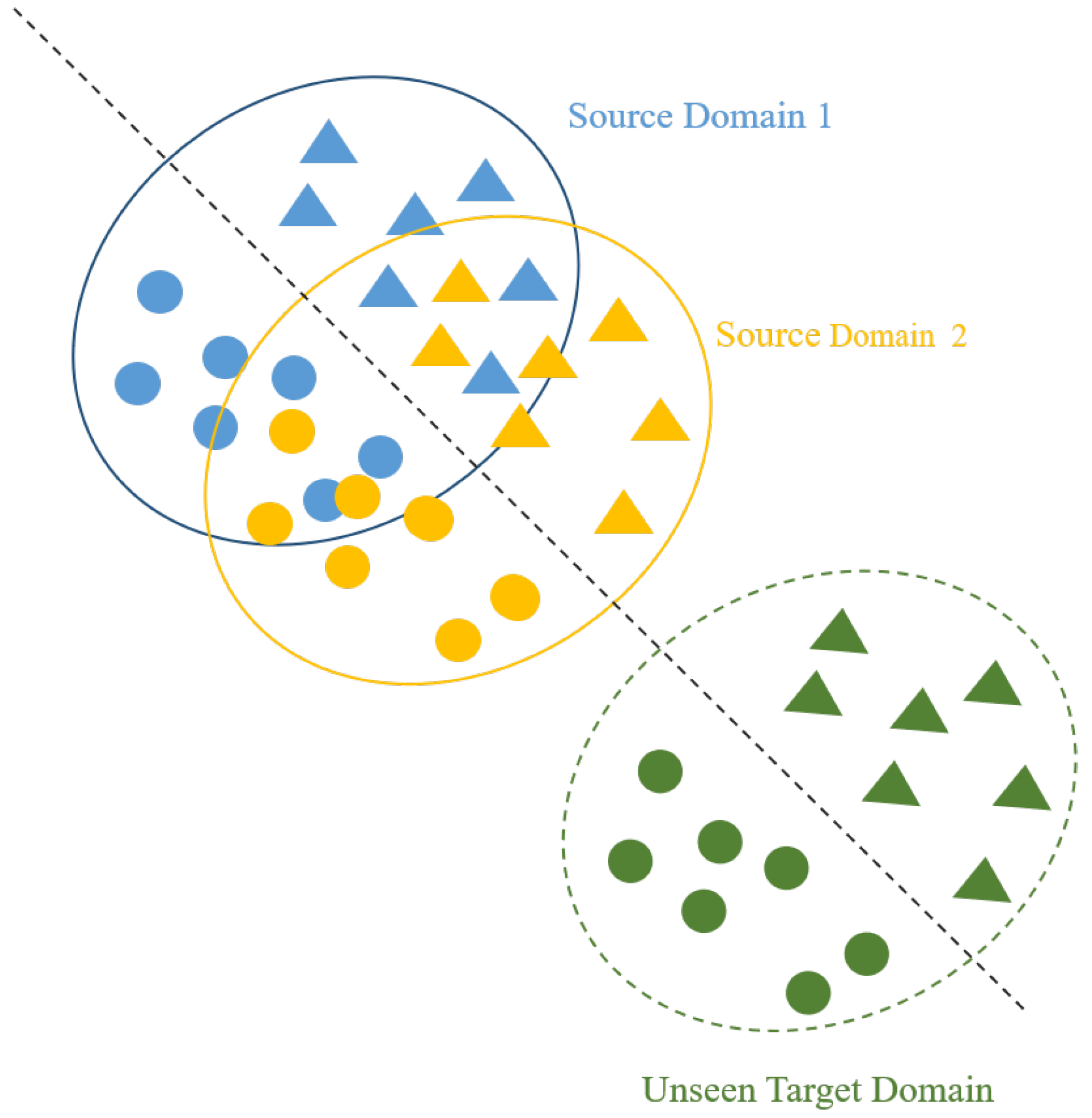
2. Brief Introduction of Domain Generalization

In domain generalization, available fault data may come from different operating conditions, such as different speeds or loads. Given M source domains ${\left\{D_m^s\right\}}_{m=1}^M$, the distributions between the source domains are different. The m-th source domain contains $n_m^s$ labeled samples $S_m^s={\{x_{m,i}^s,y_{m,i}^s\}}_{i=1}^{n_m^s}\sim D_m^s$, and the total number of source samples is $S^s={\left\{S_m^s\right\}}_{m=1}^M$. The target domain is $D^t$, the source domain is $D^s$, and the samples of the target domain are unseen during model construction and training process. The data distributions between the source and target domains are different, $D^s\ne D^t$. The goal of domain generalization networks is to learn an effective fault classification function from multiple known source domains, with available training samples ${\left\{S_m^s\right\}}_{m=1}^M$. This domain generalization network is then directly applied to the target domain with unseen operating conditions.

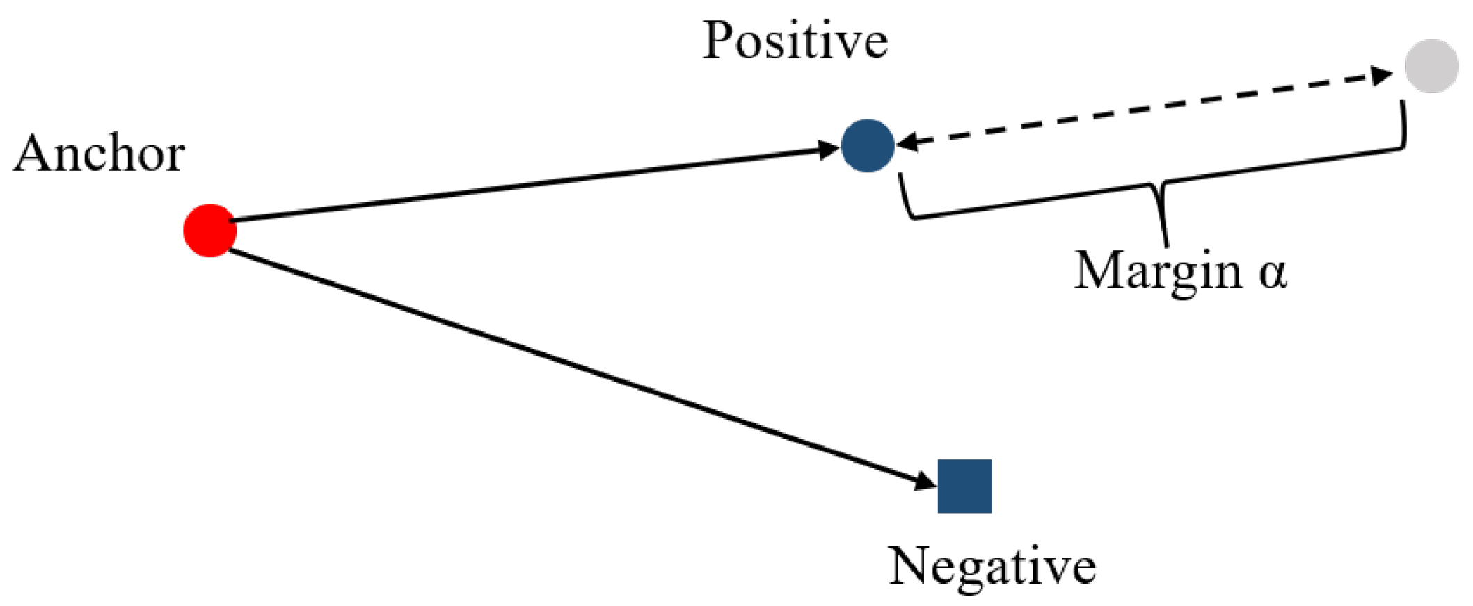
3. The Triplet Loss for Domain Generalization

Triplet loss is an effective loss in contrastive learning. The sketch of the triplet loss is given in Figure 3.

Triplets are composed of three samples, including the anchor sample $x_i^a$, the positive sample $x_j^p$, and the negative sample $x_k^n$. Among them, the anchor sample and the positive sample belong to the same category, while the anchor sample and the negative sample belong to different categories. The optimization goal of triplet loss is to reduce the distance between the anchor sample and the positive sample while increasing the distance between the anchor sample and the negative sample and can be represented as Equation (1).

$$\begin{array}{c}\hfill \parallel f\left(x_i^a\right)-f\left(x_j^p\right){\parallel }_2^2+\alpha <{\parallel f\left(x_i^a\right)-f\left(x_k^n\right)\parallel }_2^2\end{array}$$

(1)

$\forall (f\left(x_i^a\right),f\left(x_j^p\right),f\left(x_k^n\right))\in T$, where T is the set of all triplets, $\alpha$ is the margin value, $\alpha >0$, $f(·)$ is a deep neural network-based feature extractor. For each anchor sample, when forming a triplet, positive and negative samples are selected through traversal. However, not all arbitrary sets of three samples can form a triplet; two conditions must be satisfied:

(1)

$i,j,k$ are not equal, meaning all three samples are different.

(2)

The anchor sample and the positive sample belong to the same category, while the anchor sample and the negative sample belong to different categories.

Then, the triplet loss can be given as Equation (2):

$$\begin{array}{c}\hfill L_t=\sum _i^{N_{tr}}[\parallel f\left(x_i^a\right)-f\left(x_j^p\right){\parallel }_2^2-\parallel f\left(x_i^a\right)-f\left(x_k^n\right){{\parallel }_2^2+\alpha ]}_{+}\end{array}$$

(2)

where $N_{tr}$ represents the number of triplets, ${\parallel \ast \parallel }_2^2$ indicates the squared Euclidean distance, [∗]₊ indicates taking ∗ when $\ast >0$ and taking 0 when $\ast <0$. The margin value $\alpha$ can avoid projecting all samples to the same point in the feature space, i.e., $L_t=0$. Meanwhile, $\alpha$ also affects the size of the triplet loss, aiming to minimize the loss during training iterations. That is to say, the objective is to bring the anchor sample closer to the positive sample and farther from the negative sample. The choice of $\alpha$ can be analyzed as follows:

(1)

When $\alpha$ is smaller, the loss tends to approach 0 more easily. In this case, the anchor sample does not need to be pulled too close to the positive sample, and the anchor sample does not need to be pulled too far from the negative sample to quickly approach a loss of 0. However, the result obtained from such training may not effectively distinguish samples with different labels.

(2)

When $\alpha$ is larger, the network parameters need to work harder to reduce the distance between the anchor sample and the positive sample while increasing the distance between the anchor sample and the negative sample. Setting the margin value too large may result in the loss, maintaining a relatively large value, making it difficult to approach 0.

Therefore, setting a reasonable margin value is crucial, as it is an important parameter of the loss function. In summary, a smaller margin value makes the loss approach 0 more easily but may struggle to differentiate similar samples. A larger margin value makes it harder for the loss to approach 0 and may even lead to the network not converging, but it can more confidently differentiate relatively similar samples.

There are three types of triplets formed by samples: easy triplets, semi-hard triplets, and hard triplets. The distinctions among them are as follows.

The distance relationship among the three samples of easy triplets is given in Equation (3). The diagram of easy triplets is shown in Figure 4. Here, the distance between the anchor sample and the positive sample, plus $\alpha$, is smaller than the distance between the anchor sample and the negative sample. In this situation, such triplets have no impact on the total triplet loss.

$$\begin{array}{c}\hfill \parallel f\left(x_i^a\right)-f\left(x_j^p\right){\parallel }_2^2+\alpha <{\parallel f\left(x_i^a\right)-f\left(x_k^n\right)\parallel }_2^2\end{array}$$

(3)

The distance relationship among the three samples of semi-hard triplets is given in Equation (4). The diagram of semi-hard triplets is shown in Figure 5. Here, the distance between the anchor sample and the positive sample is smaller than the distance between the anchor sample and the negative sample. However, the sum of the distance between the anchor sample and the positive sample, and $\alpha$ is larger than the distance between the anchor sample and the negative sample. In this case, the semi-hard triplets have an impact on the triplet loss.

$$\begin{array}{c}\hfill \parallel f\left(x_i^a\right)-f\left(x_j^p\right){\parallel }_2^2<{\parallel f\left(x_i^a\right)-f\left(x_k^n\right)\parallel }_2^2\\ \hfill <\parallel f\left(x_i^a\right)-f\left(x_j^p\right){\parallel }_2^2+\alpha \end{array}$$

(4)

The distance relationship among the three samples of hard triplets is given in Equation (5). The diagram of hard triplets is shown in Figure 6. Here, the distance between the anchor sample and the positive sample is larger than the distance between the anchor sample and the negative sample. In this situation, the hard triplets have a significant impact on the triplet loss.

$$\begin{array}{c}\hfill \parallel f\left(x_i^a\right)-f\left(x_j^p\right){\parallel }_2^2>{\parallel f\left(x_i^a\right)-f\left(x_k^n\right)\parallel }_2^2\end{array}$$

(5)

Since easy triplets have no impact on triplet loss, to expedite the training speed of the network, attention is focused only on semi-hard triplets and hard triplets during training.

4. The Proposed TL-DGN Method for Unseen Domain Fault Diagnosis

Firstly, the triplet loss-based domain generalization network structure (TL-DGN) is constructed and illustrated in Figure 7. The TL-DGN consists of a feature extractor and a classifier. The feature extractor utilizes a one-dimensional convolutional neural network (CNN). The classifier employs two fully connected layers. Multi-source domain signals are input to the feature extractor. Then, the features extracted by the feature extractor are used to calculate the triplet loss without considering the source domain of the samples. The features are further input to the classifier, and the classification loss is computed for multi-source domains.

The loss function of TL-DGN can be given as in Equation (6):

$$\begin{array}{c}\hfill J=J_c+\beta J_{tr}\end{array}$$

(6)

where $J_c$ represents the classification loss of multi-source domains, $\beta$ is a weight coefficient. A larger $\beta$ indicates that the network pays more attention to the triplet loss. $J_{tr}$ represents the triplet loss. $J_c$ and $J_{tr}$ can be represented as Equations (7) and (8):

$$\begin{array}{ccc}\hfill & & J_c=\sum _{m=1}^M{J}_{ce}({\widehat{y}}_m,y_m)\hfill \\ & & J_{tr}=L_t\hfill \end{array}$$

(7)

$$\begin{array}{ccc}\hfill & =& \sum _i^{Ntr}[\parallel f\left(x_i^a\right)-f\left(x_j^p\right){\parallel }_2^2-\parallel f\left(x_i^a\right)-f\left(x_k^n\right){{\parallel }_2^2+\alpha ]}_{+}\hfill \end{array}$$

(8)

where $J_{ce}(·)$ is the cross-entropy loss, M is the number of source domains, ${\widehat{y}}_m$ and $y_m$, respectively, represent the classification result and the true label of fault data on the m-th source domain.

Then, the TL-DGN method can be applied to an unseen domain-bearing fault diagnosis. In real fault diagnosis scenarios, when the training sample and the test sample are not under the same load, and the load information of the test sample is unknown, the fault diagnosis model is always ineffective. To deal with the problem, TL-DGN is used for fault diagnosis of unseen domain bearings. Here, in addition to focusing on the classification loss measured by cross-entropy loss, triplet loss is used to consider the feature distribution of samples. This encourages similar samples to be close to each other and dissimilar samples to be separated, resulting in a more generalized classification boundary. The TL-DGN method for unseen domain bearing fault diagnosis has the following characteristics.

(1)

Discrimination: Firstly, the TL-DGN method can discriminate between fault features of different categories. Moreover, based on cross-entropy loss, the model can achieve low classification errors on fault data.

(2)

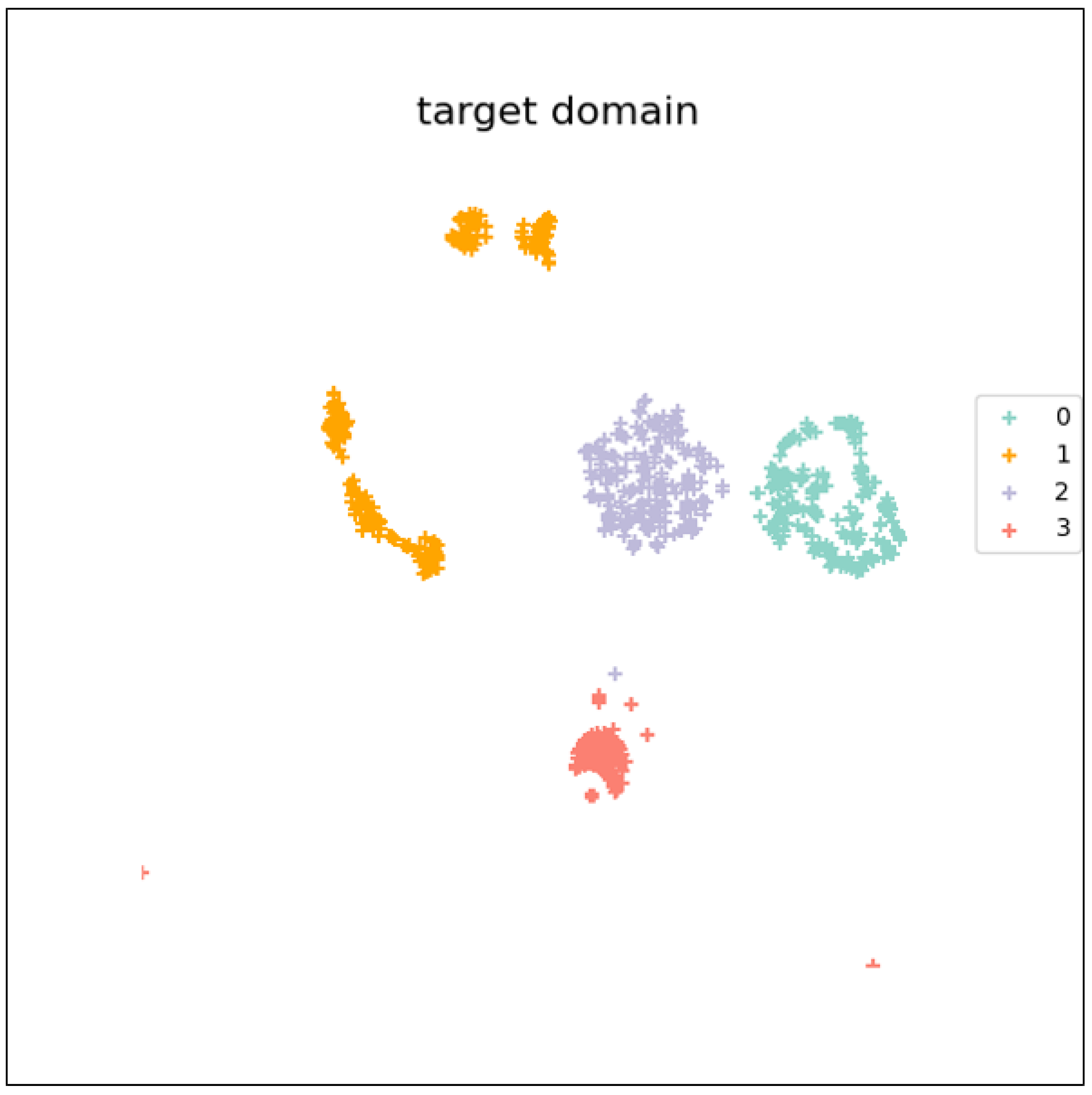
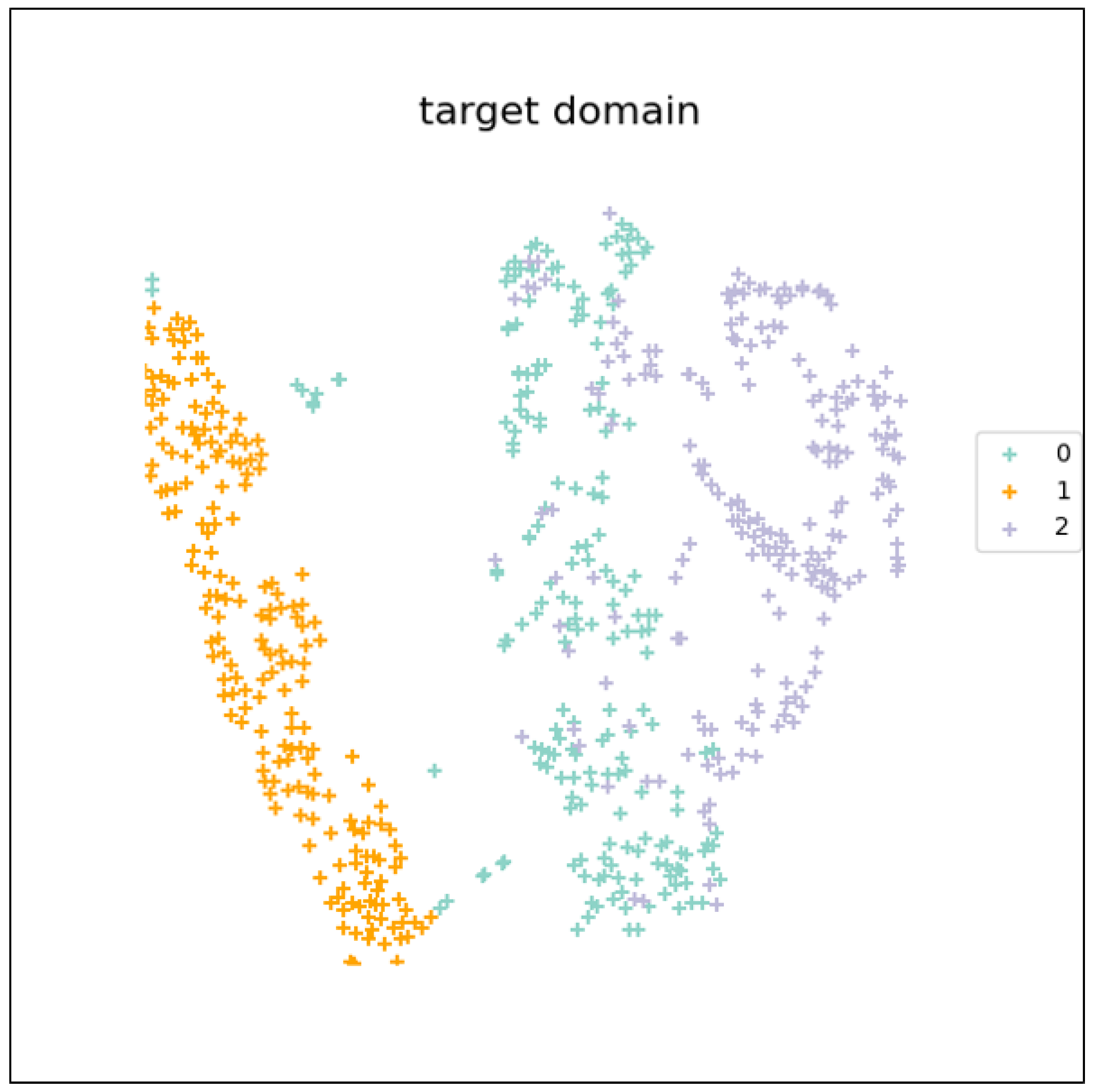
Feature clustering: In addition to classifying features, the introduced triplet loss allows features of similar fault data to cluster together, while features of dissimilar fault data are dispersed. This leads to a more discriminative classification boundary.

(3)

Generalization: Due to the discrimination and feature clustering characteristics of the proposed model, it can classify faults of different categories and aggregate features of the same category. This enhances the model’s generalization capability, making it relatively insensitive to changes in the load conditions.

The detailed process of the TL-DGN method for unseen domain-bearing fault diagnosis can be given as follows:

(1)

Collect vibration signals of bearing fault states under multiple loads as fault datasets from multi-source domains.

(2)

Establish the TL-DGN model based on Equation (6). In this model, the feature extractor is CNN, the activation function is ReLU, and the optimizer is Adam.

(3)

Divide the source domain datasets into equal-length segments. Input the vibration data from multi-source domains into the model for training while keeping the model parameters fixed.

(4)

Collect vibration signals from the target domain (signals from the target domain were not involved in the training phase). Input these signals into the trained model to obtain the diagnosis results for rolling bearing faults in the target domain.

The flowchart of the TL-DGN method for unseen domain-bearing fault diagnosis is shown in Figure 8.

5. Case Study

5.1. German Paderborn Bearing Data Set

In this section, the German Paderborn bearing data set [28] is utilized to verify the effectiveness of the proposed algorithm. The data set contains four types of loads. Among them, the rotational speed of the drive system, the radial force exerted on the test bearing, and the load torque are the main load-related operating parameters. During each measurement and acquisition process, the three parameters remain unchanged. The description of these loads is shown in

Table 1. Description of loads.

Date Set	Rotational Speed (rpm)	Load Torque (Nm)	Radial Force (N)	Name
A	1500	0.7	400	N15_M07_F04
B	1500	0.1	1000	N15_M01_F10
C	900	0.7	1000	N09_M07_F10
D	1500	0.7	1000	N15_M07_F10

.

In this paper, four categories of faults, KI01, KA01, KA07, and KI03, were chosen for the diagnosis experiment. To simplify the description, datasets with load names N15_M07_F04, N15_M01_F10, N09_M07_F10, and N15_M07_F10 are respectively referred to as datasets A, B, C, and D. Bearing damage includes two types: artificial damage and real damage. Both types of damage are applied to the inner and outer races of the 6203 model bearings. Here, artificial damage includes three types: electro-discharge machining (with a groove length of 0.25 mm in the rolling direction and a depth of 1–2 mm), drilling (with diameters of 0.9 mm, 2 mm, and 3 mm), and manual electric engraving (damage lengths ranging from 1–4 mm). Detailed information about artificially damaged bearings is provided in

Table 2. Description of faults.

Bearing Code	Module	Damage Degree	Damage Mode
KI01	IR	1	Electro discharge machining
KA01	OR	1	Electro discharge machining
KA07	OR	1	Drilling
KI03	IR	1	Electric engraving

, where OR refers to the outer race and IR refers to the inner race.

Here, fault signals in each category were partitioned into segments of length 1024, with 1000 samples for each fault category. In this experiment, the training and testing sets were split in an 8:2 ratio for each load. The data sets under each load are shown in

Table 3. Experimental data set.

Fault Category	Label	Number of Sample	Dimension of Sample
KI01	0	1000	1 × 1024
KA01	1	1000	1 × 1024
KA07	2	1000	1 × 1024
KI03	3	1000	1 × 1024

.

The structure and parameters of the proposed model are shown in

Table 4. Model structure and parameters.

	Layer	Parameter
	Input	/	/
	Conv1D_1	kernel_size = 11, filters = 32	ReLU
	MaxP_2	pool_size = 11	/
Feature	Conv1D_3	kernel_size = 5, filters = 32	ReLU
Extractor	MaxP_4	pool_size = 5	/
	Conv1D_5	kernel_size = 3, filters = 16	ReLU
	AverP_6	pool_size = 3	/
	Dropout	0.5	/
Label	FC1	50	ReLU
Classifier	FC2	4	Softmax

. The experiment was undertaken under the Python 3.9 (pytorch) framework. The number of iterations was set to 50, the sample batch size was set to 128, the optimizer was Adam. The initial learning rate was set to 0.005 and adjusted according to exponential decay during the iteration process.

In order to verify the effectiveness of triplet loss, an experiment was first conducted with data set A. The training set of data set A was input into the model for network training, and the testing set of data set A was used to obtain the diagnosis results. Use t-SNE to observe the difference in feature distribution when the model was trained with triplet loss and without triplet loss. The feature visualizations of data set A are given in Figure 9 and Figure 10. In the experiment, considering the convergence speed of the model, in each round of iteration, for each anchor point sample, the nearest negative sample and the farthest positive sample are selected to form the hardest triplet to participate model optimization.

In this case, the margin $\alpha$ of the triplet loss was set to 10, and the weight parameter $\beta$ of the triplet loss was set to 0.1. Adding or not adding triplet loss into the loss function, the model distributions obtained from the test set of data set A showed a noticeable difference. The same category of data in Figure 9 was not as clustered as in Figure 10.

Then, the domain generalization comparison experiment with and without adding triplet loss was conducted. Similarly, in this experiment, the margin $\alpha$ of the triplet loss was set to 10, and the weight parameter $\beta$ of the triplet loss was set to 0.1. The fault diagnosis accuracy results of the model with and without adding triplet loss are shown in

Table 5. Accuracy of the model in the generalization experiment (%).

Source Domain	Target Domain	With Triplet Loss	Without Triplet Loss
A,B	C	70.02	69.15
A,B	D	99.97	99.97
A,C	B	98.67	97.77
C,D	A	96.52	94.02
C,D	B	99.45	97.50
A,C	D	99.22	99.02
Average		93.98	92.91

. In Table 5, the source domain column represents the data set participating in the training process, and the target domain column is the data set that cannot participate in the training process, that is, the unseen domain. For example, if the source domains are A and B, and the target domain is C, it indicates that the model was trained using datasets A and B, and tested on dataset C. In order to mitigate the randomness of diagnostic results, each experiment was repeated five times, and the results in Table 5 are the average of five repetitions.

With the addition of triplet loss, it has a higher fault diagnosis accuracy in the unseen target domain compared to the contrast experiments. However, in the generalization task between different loads, when the target domain is C, both the proposed method and the comparative methods have lower fault diagnosis accuracy compared to other tasks. This is attributed to the significant differences between data set C and the others. Data set C was collected at a driving system speed of 900 rpm, while the other three data sets were collected at a speed of 1500 rpm. When the A, B, and D data sets were used as target domains, the proposed algorithm achieved higher accuracy in the target domain. Judging from the average value of the six generalization tasks, the fault diagnosis accuracy obtained by the proposed method was higher than that of the comparative experiment.

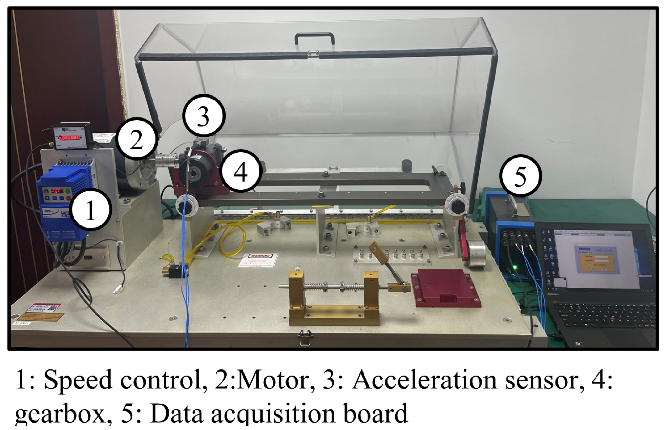
5.2. HUSTgearbox Data Set

The HUSTgearbox data set is publicly available from Huazhong University of Science and Technology and consists of gearbox data [29]. Gearbox fault testing was conducted using the Spectra-Quest mechanical fault simulator. There are three health states for the gearbox: Normal, Tooth broken, and Tooth missing, labeled 0, 1, 2. Test rig of HUSTgearbox dataset is shown in Figure 11. Photographs of the failure gears are given in Figure 12. In the experiment, a total of four different operating conditions were set. The operating conditions (rotating speed and load) include: A: 20 Hz and 0.113 Nm; B: 25 Hz and 0.226 Nm; C: 30 Hz and 0.339 Nm; D: 35 Hz and 0.452 Nm. Under each operating condition, 1000 samples were selected for each health state, divided into training and testing sets in an 8:2 ratio. Here, the three health states of conditions A, B, and C were used as the training set, while the three states of condition D were used as the testing set to validate domain generalization effects.

In this case, the margin $\alpha$ of the triplet loss was set to 5, and the weight parameter $\beta$ of the triplet loss was set to 0.001, 0.002, and 0.005. For the TL-DGN model, the number of iterations was set to 100, the sample batch size was set to 50, and the optimizer was Adam. The proposed model was compared with the KNN [30] and support vector machine (SVM) [31] methods, classification model without triplet loss ($\beta =0$), and $\beta =0.01$, 0.02, and 0.05. The experimental results are given in

Table 6. Accuracy of the model in the generalization experiment (%).

	KNN	SVM	Without Triplet Loss	$\mathit{\beta }=0.01$	$\mathit{\beta }=0.02$	$\mathit{\beta }=0.05$
Accuracy	0.3783	0.5050	0.6540	0.7556	0.7254	0.7238

.

Figure 13, Figure 14, Figure 15 and Figure 16 present feature visualizations of data set D.

From Table 6 and Figure 13, Figure 14, Figure 15 and Figure 16, it can be observed that introducing triplet loss to some extent enables different class samples in the target domain to be more dispersed, while samples of the same class are more aggregated, thereby improving the prediction accuracy of the model.

6. Conclusions

This paper innovatively introduces the TL-DGN model. In this method, in addition to focusing on the classification loss measured by cross-entropy loss, triplet loss is used to consider the feature distribution of samples. This encourages similar samples to be close to each other and dissimilar samples to be separated, resulting in a more generalized classification boundary. Through two comparison experiments with fault diagnosis models without triplet loss and other models, the proposed model in this paper achieved the best fault diagnosis performance. It can be observed that directly applying the model trained by multi-source domain data to fault diagnosis in unseen domains achieves poor results. However, the model based on triplet loss introduces contrastive learning principles, which can reduce the distance between samples of the same class from different domains and can be extended to unseen domains. From multiple feature visualization figures, it can be seen that after incorporating triplet loss, there is a certain improvement in the clustering effect in the target domain.

References

1. Edwards, S.; Lees, A.W.; Friswell, M.I. Fault diagnosis of rotating machinery. Shock Vib. Dig. 1998, 30, 4–13. [Google Scholar] [CrossRef]
2. Liu, R.; Yang, B.; Zio, E.; Chen, X. Artificial intelligence for fault diagnosis of rotating machinery: A review. Mech. Syst. Signal Process. 2018, 108, 33–47. [Google Scholar] [CrossRef]
3. Wang, T.; Han, Q.; Chu, F.; Feng, Z. Vibration based condition monitoring and fault diagnosis of wind turbine planetary gearbox: A review. Mech. Syst. Signal Process. 2019, 126, 662–685. [Google Scholar] [CrossRef]
4. Lei, Y.; Lin, J.; He, Z.; Zuo, M.J. A review on empirical mode decomposition in fault diagnosis of rotating machinery. Mech. Syst. Signal Process. 2013, 35, 108–126. [Google Scholar] [CrossRef]
5. Tao, H.; Wang, P.; Chen, Y.; Stojanovic, V.; Yang, H. An unsupervised fault diagnosis method for rolling bearing using STFT and generative neural networks. J. Frankl. Inst. 2020, 357, 7286–7307. [Google Scholar] [CrossRef]
6. Peng, Z.K.; Chu, F. Application of the wavelet transform in machine condition monitoring and fault diagnostics: A review with bibliography. Mech. Syst. Signal Process. 2004, 18, 199–221. [Google Scholar] [CrossRef]
7. Zheng, H.; Li, Z.; Chen, X. Gear fault diagnosis based on continuous wavelet transform. Mech. Syst. Signal Process. 2002, 16, 447–457. [Google Scholar] [CrossRef]
8. Yu, Y.; Junsheng, C. A roller bearing fault diagnosis method based on EMD energy entropy and ANN. J. Sound Vib. 2006, 294, 269–277. [Google Scholar] [CrossRef]
9. Chen, X.S.; Zeng, H.B.; Li, Z.X. A multi-fault diagnosis method of rolling bearing based on wavelet-PCA and fuzzy K-nearest neighbor. Appl. Mech. Mater. 2010, 29, 1602–1607. [Google Scholar] [CrossRef]
10. Wang, Z.; Zhang, Q.; Xiong, J.; Xiao, M.; Sun, G.; He, J. Fault diagnosis of a rolling bearing using wavelet packet denoising and random forests. IEEE Sens. J. 2017, 17, 5581–5588. [Google Scholar] [CrossRef]
11. Li, X.; Zhang, W.; Ding, Q.; Li, X. Diagnosing rotating machines with weakly supervised data using deep transfer learning. IEEE Trans. Ind. Inform. 2019, 16, 1688–1697. [Google Scholar] [CrossRef]
12. Wang, X.; Qin, Y.; Wang, Y.; Xiang, S.; Chen, H. ReLTanh: An activation function with vanishing gradient resistance for SAE-based DNNs and its application to rotating machinery fault diagnosis. Neurocomputing 2019, 363, 88–98. [Google Scholar] [CrossRef]
13. Pan, H.; He, X.; Tang, S.; Meng, F. An improved bearing fault diagnosis method using one-dimensional CNN and LSTM. J. Mech. Eng. Vestn. 2018, 64, 443–452. [Google Scholar]
14. Hoang, D.T.; Kang, H.J. A survey on deep learning based bearing fault diagnosis. Neurocomputing 2019, 335, 327–335. [Google Scholar] [CrossRef]
15. Wang, D.; Guo, Q.; Song, Y.; Gao, S.; Li, Y. Application of multiscale learning neural network based on CNN in bearing fault diagnosis. J. Signal Process. Syst. 2019, 91, 1205–1217. [Google Scholar] [CrossRef]
16. Niu, G.; Wang, X.; Golda, M.; Mastro, S.; Zhang, B. An optimized adaptive PReLU-DBN for rolling element bearing fault diagnosis. Neurocomputing 2021, 445, 26–34. [Google Scholar] [CrossRef]
17. Cui, M.; Wang, Y.; Lin, X.; Zhong, M. Fault diagnosis of rolling bearings based on an improved stack autoencoder and support vector machine. IEEE Sens. J. 2020, 21, 4927–4937. [Google Scholar] [CrossRef]
18. Nie, X.; Xie, G. A novel normalized recurrent neural network for fault diagnosis with noisy labels. J. Intell. Manuf. 2021, 32, 1271–1288. [Google Scholar] [CrossRef]
19. Wang, Y.R.; Sun, G.D.; Jin, Q. Imbalanced sample fault diagnosis of rotating machinery using conditional variational auto-encoder generative adversarial network. Appl. Soft Comput. 2020, 92, 106333. [Google Scholar] [CrossRef]
20. Ghifary, M.; Kleijn, W.B.; Zhang, M.; Balduzzi, D. Domain generalization for object recognition with multi-task autoencoders. In Proceedings of the IEEE International Conference on Computer Vision, Santiago, Chile, 7–13 December 2015; pp. 2551–2559. [Google Scholar]
21. Wang, J.; Lan, C.; Liu, C.; Ouyang, Y.; Qin, T.; Lu, W.; Chen, Y.; Zeng, W.; Philip, S.Y. Generalizing to unseen domains: A survey on domain generalization. IEEE Trans. Knowl. Data Eng. 2022, 35, 8052–8072. [Google Scholar] [CrossRef]
22. Zhou, K.; Liu, Z.; Qiao, Y.; Xiang, T.; Loy, C.C. Domain generalization: A survey. IEEE Trans. Pattern Anal. Mach. Intell. 2022, 45, 4396–4415. [Google Scholar] [CrossRef]
23. Chen, L.; Li, Q.; Shen, C.; Zhu, J.; Wang, D.; Xia, M. Adversarial domain-invariant generalization: A generic domain-regressive framework for bearing fault diagnosis under unseen conditions. IEEE Trans. Ind. Inform. 2021, 18, 1790–1800. [Google Scholar] [CrossRef]
24. Shi, Y.; Deng, A.; Deng, M.; Li, J.; Xu, M.; Zhang, S.; Ding, X.; Xu, S. Domain transferability-based deep domain generalization method towards actual fault diagnosis scenarios. IEEE Trans. Ind. Inform. 2022, 19, 7355–7366. [Google Scholar] [CrossRef]
25. Zhao, C.; Shen, W. Federated domain generalization: A secure and robust framework for intelligent fault diagnosis. IEEE Trans. Ind. Inform. 2023, 20, 2662–2670. [Google Scholar] [CrossRef]
26. Fan, Z.; Xu, Q.; Jiang, C.; Ding, S.X. Deep mixed domain generalization network for intelligent fault diagnosis under unseen conditions. IEEE Trans. Ind. Electron. 2023, 71, 965–974. [Google Scholar] [CrossRef]
27. Wang, X.; Liu, F. Triplet loss guided adversarial domain adaptation for bearing fault diagnosis. Sensors 2020, 20, 320. [Google Scholar] [CrossRef]
28. Lessmeier, C.; Kimotho, J.K.; Zimmer, D.; Sextro, W. Condition monitoring of bearing damage in electromechanical drive systems by using motor current signals of electric motors: A benchmark data set for data-driven classification. In Proceedings of the PHM Society European Conference, Bilbao, Spain, 5–8 July 2016; Volume 3. [Google Scholar]
29. Zhao, C.; Zio, E.; Shen, W. Domain Generalization for Cross-Domain Fault Diagnosis: An Application-oriented Perspective and a Benchmark Study. Reliab. Eng. Syst. Saf. 2024, 245, 109964. [Google Scholar] [CrossRef]
30. Sanchez, R.V.; Lucero, P.; Vasquez, R.E.; Cerrada, M.; Macancela, J.C.; Cabrera, D. Feature ranking for multi-fault diagnosis of rotating machinery by using random forest and KNN. J. Intell. Fuzzy Syst. 2018, 34, 3463–3473. [Google Scholar] [CrossRef]
31. Jing, C.; Hou, J. SVM and PCA based fault classification approaches for complicated industrial process. Neurocomputing 2015, 167, 636–642. [Google Scholar] [CrossRef]
Figure 1. Sketch of domain adaptation (circles and triangles represent two different categories).
Processes 12 00882 g001
Figure 2. Sketch of domain generalization (circles and triangles represent two different categories).
Processes 12 00882 g002
Figure 3. Sketch of triplet loss.
Processes 12 00882 g003
Figure 4. The diagram of easy triplets.
Processes 12 00882 g004
Figure 5. The diagram of semi-hard triplets.
Processes 12 00882 g005
Figure 6. Diagram of the hard triplet.
Processes 12 00882 g006
Figure 7. Network structure of the triplet loss-based domain generalization network (TL-DGN).
Processes 12 00882 g007
Figure 8. Flowchart of the triplet loss-based domain generalization network (TL-DGN) method.
Processes 12 00882 g008
Figure 9. Feature visualization of data set A (without triplet loss).
Processes 12 00882 g009
Figure 10. Feature visualization of data set A (triplet loss-based domain generalization network (TL-DGN)).
Processes 12 00882 g010
Figure 11. Test rig of HUSTgearbox dataset [29].
Processes 12 00882 g011
Figure 12. Photographs of the failure gears [29].
Processes 12 00882 g012
Figure 13. Feature visualization of data set D (without triplet loss).
Processes 12 00882 g013
Figure 14. Feature visualization of data set D (triplet loss-based domain generalization network (TL-DGN), β = 0.001 ).
Processes 12 00882 g014
Figure 15. Feature visualization of data set D (triplet loss-based domain generalization network (TL-DGN), β = 0.002 ).
Processes 12 00882 g015
Figure 16. Feature visualization of data set D (triplet loss-based domain generalization network (TL-DGN), β = 0.005 ).
Processes 12 00882 g016