Trajectory Tracking Control of Mobile Manipulator Based on Improved Sliding Mode Control Algorithm

Abstract

Research on trajectory tracking control for climbing welding robots holds significant importance in the field of automated welding. However, existing trajectory tracking methods suffer from issues such as jitter and slow speed. In this paper, an improved sliding mode control strategy is proposed based on the self-designed wall-climbing welding mobile manipulator. Firstly, a new adaptive sliding mode control strategy is proposed for the mobile platform based on the kinematic model. By introducing a new approach law, the controller is designed when the distance between the center of mass is unknown. Secondly, regarding the manipulator, we analyze simplified dynamic equations, extract uncertain components, and utilize a CNN for compensation. This compensation strategy is integrated into the sliding mode control law, achieving precise control over the manipulator and effectively resolving issues like slow tracking speeds, large errors, and chattering. The stability of the robot control system is proved by the Lyapunov function. Through simulation analysis and experimental validation, the proposed control method is confirmed to be feasible and superior.

1. Introduction

As one of the most widely used industrial robots, the climbing wall welding manipulator is an indispensable component in the automated welding operations of large-scale engineering structures, large storage tanks, ships, offshore platforms, large-diameter pipelines, and other equipment [1,2]. The harsh working environment, low efficiency, and unstable welding quality highlight the crucial significance and substantial economic value of designing efficient welding manipulators [3,4].

Researchers have conducted extensive studies on the structural design of robots [5,6,7,8]. Nagano et al. [9] designed a wheel-legged hybrid robot featuring four legs, each equipped with two shock absorbers and two joints, with wheels acting as feet. While the robot demonstrates adaptability to various types of rough and uneven ground, challenges arise when transitioning to the hull plate, particularly regarding the installation and stability of the adsorption device. Gui et al. [10] proposed a novel intelligent wall-climbing welding robot system for large steel structure manufacturing. The manipulator comprises a crosshead slipper and a swing device. While it can meet the working requirements, its flexibility is not sufficient. The climbing wall welding mobile manipulator is the most advanced type of welding robot, composed of one or more manipulator arms with operational capabilities and a mobile platform providing movement capabilities [11,12,13]. The sliding mode control (SMC), as a method for controlling nonlinear systems, is successful primarily due to its robustness against structured and unstructured uncertainties, as well as its ease of implementation [14]. However, the irreconcilable contradiction between chattering and tracking errors has constrained its development [15].

The speed of the mobile platform studied in this paper is relatively slow in the process of motion, and the method of the kinematics model can meet the control requirements. Variable structure sliding mode control based on the kinematic model has advantages such as simple control structure and easy implementation, but it has disadvantages such as time delay and constant switch closing in actual use, which is prone to high-frequency buffeting [16]. The control method based on the approach law can enhance the dynamic performance of the system by adjusting the parameters of the approach law and reducing buffeting. Wang et al. [17] propose a sliding mode control method based on the adaptive reaching law to maintain the good speed control performance of permanent magnet synchronous motors under internal and external disturbances. Sharaf et al. [18] designed a two-step controller for the DC microgrid using the deep neural network and sliding mode control method based on the exponential reaching law. The proposed control method uses the exponential reaching law to eliminate the chattering phenomenon and provide a fast arrival time.

Due to the nonlinear, strongly coupled, and uncertain characteristics of manipulators, the precise control of manipulators has been a challenging and focal point in the field of control [19]. Some recent studies have used the model-based NN-based SMC approach in robot control [20,21,22,23]. Duan et al. [24] proposed a neural network terminal SMC method that combines a fast non-singular terminal sliding mode control, radial basis function neural network, and improved sliding mode particle swarm optimization, which effectively improves the trajectory tracking accuracy of the manipulator under the influence of uncertain factors. Liu et al. [25] proposed a sliding mode control scheme of neural networks based on iterative learning, which, for the first time, incorporated the concept of iterative learning into the sliding mode control method of neural networks. The uncertainty and disturbance are compensated by the complementary neural network and iterative learning, and the motion performance of repetitive tasks is improved [26]. The use of CNN for the precise compensation of uncertain components in the manipulator model can mitigate the chattering drawbacks associated with traditional sliding mode control [27]. Due to the presence of operations such as convolution, these networks exhibit stronger learning capabilities compared to traditional radial basis function (RBF) neural network models [28]. This leads to a further improvement in tracking accuracy and the avoidance of delay estimation based on empirical data learning control laws.

The objective of this study is to design a novel climbing wall welding mobile manipulator and provide a more precise control method for the robot. The main tasks and contributions of this paper are outlined as follows:

• Designing a novel robot structure featuring a hybrid wheel-leg mobile platform, a non-contact variable magnetic adhesion mechanism, and a more flexible 5-DOF manipulator. This configuration endows the robot with enhanced operational capabilities, meeting the requirements of a wide range of tasks.
• A novel adaptive SMC strategy based on the kinematic model is proposed for the mobile platform. By introducing a novel reaching law, the controller is designed considering the unknown distance from the center of mass, and the stability is proved by the Lyapunov function.
• Introducing a control method for the trajectory tracking of the manipulator using a combination of a neural network and SMC. Initially, the dynamic model of the manipulator is analyzed, and the uncertain components are extracted. Subsequently, a CNN is designed to compensate for these uncertainties. The compensation terms are then incorporated into the SMC, enabling improved trajectory tracking through the refined SMC approach.

The remaining structure of this paper is outlined as follows: Section 2 introduces the overall structure of the robot; Section 3 designs the sliding mode controller for the mobile platform, and the robot arm, respectively; Section 4 verifies that the robot can basically achieve the functional requirements through simulation analysis and experiments; Section 5 introduces the conclusion.

2. Robot Design

2.1. Design Requirements

The designed wall-climbing welding mobile manipulator in this paper finds its primary application in the welding, testing, and maintenance of extensive ship surfaces or other large non-structural equipment. Through field investigations and analysis, we identified that the operating environment exhibits characteristics such as a large area, substantial curvature, and harsh conditions. Several considerations, encompassing robot structural design, operational requirements, and other specifications, need to be addressed, covering the following aspects:

(1)

Reliable load capacity. Due to the need to carry complex welding equipment for welding operations, to ensure flexible operation on different curvature walls, the robot needs to have sufficient load capacity while overcoming its own gravity.

(2)

Smooth obstacle-crossing ability. There are many obstacles on the working surface, such as sinews, welds, and grooves, and the robot needs to adapt to the environment and cross the inevitable obstacles in the process of movement.

(3)

Good control performance. In the process of operation, the robot needs to achieve wall climbing, obstacle crossing, movement or turning, and other functions and needs to realize welding operations through the robot arm. It is necessary to design a reliable control method while meeting the requirements of robot movement flexibility and safety.

In accordance with the analysis of the issues and design requirements, the primary technical parameters of the wall-climbing welding mobile manipulator are presented in

Table 1. Main technical parameters.

Design Index	Value/Type
Power type	Electric drive
Adsorption mechanism	Permanent non-contact magnet
Obstacle crossing mechanism	Electric lifting platform
Welding actuator	5-DOF manipulator
Body size/(mm)	780 × 300 × 450
Machine weight/(kg)	80
Maximum moving speed/(mm/min)	1800
Load capacity/(N)	200
Size of obstacles to cross/(mm)	90×90
Welding process	K-TIG

below.

2.2. Mechanical Structure and Working Principle

Combining examples of wheeled-leg hybrid robots operating on the ground, we propose a rational and efficient climbing wall welding mobile manipulator. The prototype is illustrated in Figure 1.

The mechanical structure and working principles are outlined as follows:

1. The robot’s legs consist of three electric lifting platforms installed on the abdomen, fixed beneath the top universal mounting plate. When the robot encounters unavoidable obstacles, the legs sequentially lift the structure of the wheels to overcome the obstacles, as depicted in Figure 2, (a–c) is the obstacle crossing process of the front wheel, (d–f) is the obstacle crossing process of the middle wheel, and (g–i) is the obstacle crossing process of the rear wheel. The robot can traverse obstacles up to a maximum height of 90 mm.

2. The wheel structure comprises six wheels, individually controlled by inner brushless DC servo motors. Connected to the top universal plate through elastic telescopic columns, the wheel structure can adapt to certain curved surfaces. The robot lacks a steering mechanism and achieves steering through differential wheel speed, as illustrated in Figure 3.

3. Magnets are installed beneath the motors to ensure the robot’s wall-climbing capability. Additionally, they can move up and down with the lifting of the legs, allowing for the adjustment of the magnetic force.

4. A laser radar and binocular camera are positioned at the front of the robot, enabling obstacle detection and environmental observation. Additional sensors are internally placed in the robot based on operational requirements.

5. Drivers, relays, control circuit boards, and other components are securely mounted on the universal mounting plate, significantly saving space.

6. The 5-DOF manipulator is installed on the exterior of the mobile platform shell. The first degree of freedom employs a rotary joint, while the second, third, and fourth degrees of freedom utilize pitch joints. The fifth degree of freedom adopts a rotary joint. This configuration effectively enhances the flexibility of trajectory planning within the local workspace for welding tasks. A COMS camera and K-TIG welding gun are mounted on a self-made clamping mechanism, facilitating efficient welding operations.

3. Controller Design of the Robot

The wall-climbing welding mobile robot studied in this paper is a complex redundant system composed of a moving platform and robot arm. The establishment of its kinematic mathematical model is the basis of its research and control [29,30].

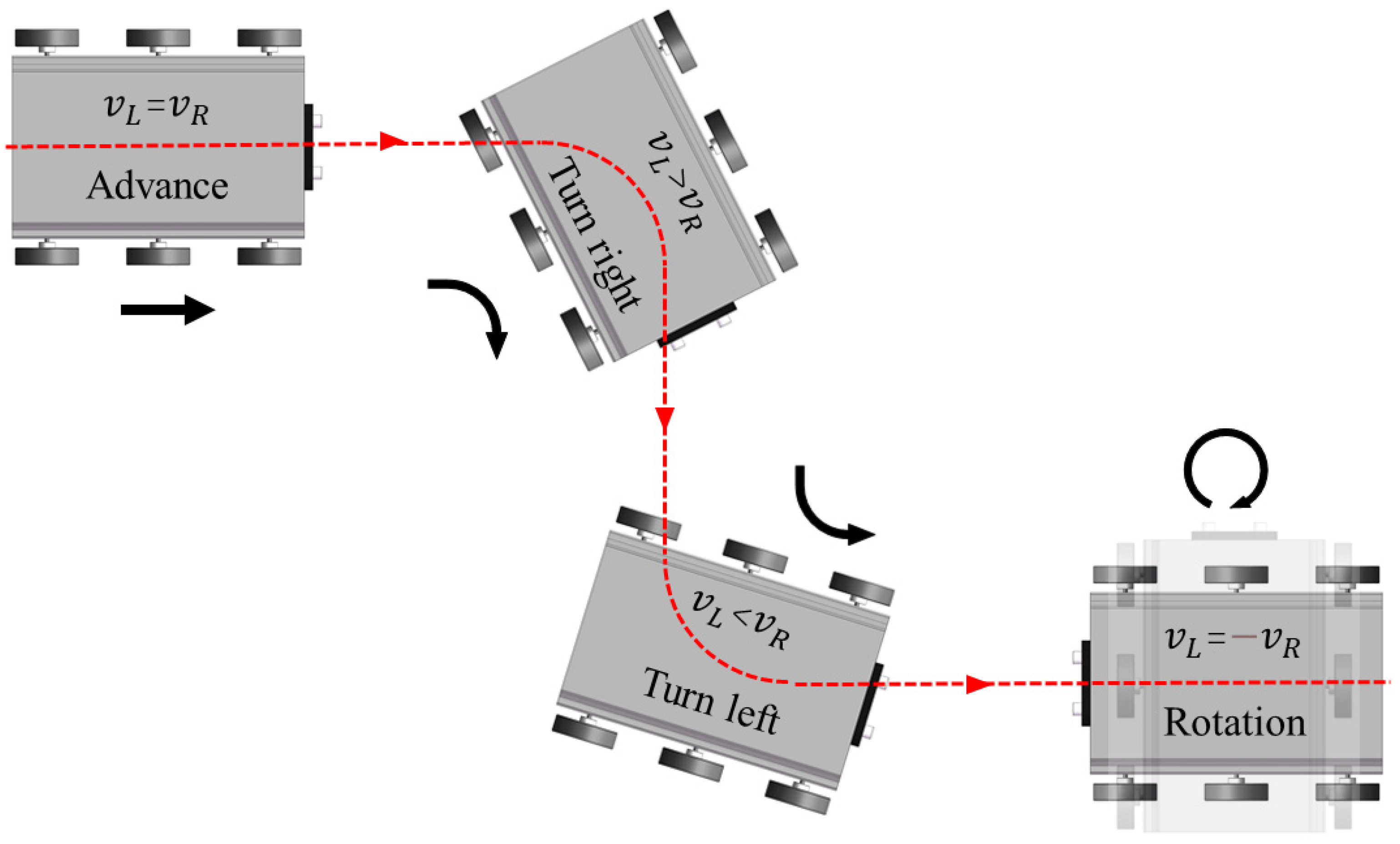
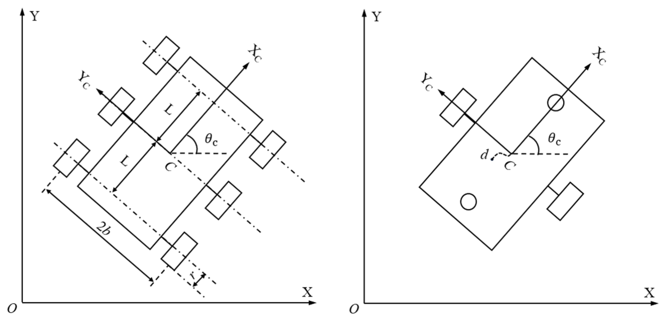
3.1. Kinematics Analysis of Mobile Platform

Due to the unique nature of the working environment, the robot is not equipped with a steering mechanism. Instead, steering is achieved through the differential motion of the left and right-side wheels. During the steering process, the mobile platform rotates around a point on the axis of the middle two wheels, with only these middle wheels rolling. The front and rear four wheels experience both lateral and radial sliding while rolling. To simplify the analysis, the front and rear wheel pairs were equivalently modeled as passive caster wheels. The differential motion is achieved through the middle two wheels, leading to a simplified two-wheel differential model, as illustrated in Figure 4. Based on this, the kinematic model of the robot is established.

$XOY$ is the geodetic coordinate system, $X_{c}C{Y}_c$ is the local coordinate system with the robot itself as the reference frame, ${\theta }_c$ representing the angle between the forward $X_c$ axis and the forward $X$ axis, that is, the yaw angle. The distance between the left and right wheels of the mobile platform is set as $2b$, and the radius of the wheels is set as $r$; $d$ is the distance between the center of mass of the robot. Let the actual linear velocity and angular velocity of the mobile platform be $v$ and $\omega$, respectively, $C$ is the geometric center of the robot, the pose coordinate in the $XOY$ coordinate system is $\left(x_c,y_c,{\theta }_c\right)$, and the actual pose of the mobile platform is expressed as follows: $q={\left[x_c,y_c,{\theta }_c\right]}^{\mathrm{T}}$.

In an ideal state, wheeled mobile robots are subject to the following non-holonomic constraints [31]:

$${\dot{y}}_c\cos {\theta }_c-{\dot{x}}_c\sin {\theta }_c-d{\dot{\theta }}_c=0$$

(1)

The robot can obtain the following kinematic model under the non-holonomic constraint (1):

$$\dot{q}=\left[\begin{array}{c}{\dot{x}}_c\\ {\dot{y}}_c\\ {\dot{\theta }}_c\end{array}\right]=\left[\begin{array}{cc}\cos {\theta }_c& -d\sin {\theta }_c\\ \sin {\theta }_c& d\cos {\theta }_c\\ 0& 1\end{array}\right]\left[\begin{array}{c}{v}_c\\ {\omega }_c\end{array}\right]$$

(2)

Given the expected linear velocity $v_d$, the expected angular velocity $w_d$, the expected pose coordinate ${(x_d,y_d,{\theta }_d)}^{\mathrm{T}}$, and the error pose $P_e={\left[x_e,y_e,{\theta }_e\right]}^{\mathrm{T}}$, the following kinematic model can be obtained:

$$P_e=\left[\begin{array}{c}{x}_e\\ y_e\\ {\theta }_e\end{array}\right]=\left[\begin{array}{ccc}\cos {\theta }_c& \sin {\theta }_c& 0\\ -\sin {\theta }_c& \cos {\theta }_c& 0\\ 0& 0& 1\end{array}\right]\left[\begin{array}{c}{x}_d-x_c\\ y_d-y_c\\ {\theta }_d-{\theta }_c\end{array}\right]$$

(3)

By combining (2) and (3), the following error equation of the robot can be obtained:

$$\{\begin{array}{l}{\dot{x}}_e={\omega }_c{y}_e+{\nu }_d\cos {\theta }_e-{\nu }_c-d{\omega }_d\sin {\theta }_e\hfill \\ {\dot{y}}_e=-{\omega }_c{x}_e+{\nu }_d\sin {\theta }_e+d{\omega }_d\cos {\theta }_e-d{\omega }_c\hfill \\ {\dot{\theta }}_e={\omega }_d-{\omega }_c\hfill \end{array}$$

(4)

The trajectory tracking control problem studied in this paper can be described as follows: design a suitable speed controller $v$ and $\omega$ so that the tracking error of the wheeled mobile robot under the action of the controller can asymptotically converge for any given initial value, that is, the modulus of the error matrix ${\left[x_e,y_e,{\theta }_e\right]}^{\mathrm{T}}$ converges to zero, then $\underset{t\to \infty }{\lim }\Vert {\left[x_e,y_e,{\theta }_e\right]}^{\mathrm{T}}\Vert =0$.

3.2. Controller Design of Mobile Platform

The mobile platform control system is a multi-input nonlinear system. The sliding mode surface is designed by combining the backstepping control algorithm. The idea is that when $x_e$ converges to 0 and ${\theta }_e$ converges to $-\arctan ({\nu }_d{y}_e)$, then $y_e$ also converges to 0, so just design the controller $[v,{\omega ]}^{\mathrm{T}}$ can produce $\underset{t\to \infty }{\lim }{x}_e=0$ and $\underset{t\to \infty }{\lim }{\theta }_e=-\arctan ({\nu }_d{y}_e)$. The switching function is given as follows:

$$s\left(P_e\right)=[\begin{array}{c}{s}_1\left(P_e\right)\\ s_2\left(P_e\right)\end{array}]=\left[\begin{array}{c}{x}_e\\ {\theta }_e+\arctan \left({\nu }_d{y}_e\right)\end{array}\right]$$

(5)

In practical applications, the typical reaching laws are the isokinetic reaching law, exponential reaching law, power reaching law, and general reaching law, but they have the disadvantages of jitter and slow convergence [32].

For the power reaching law $\dot{s}=-k|s{|}^{\alpha }\mathrm{sgn}(s)-ks$, $k>0$, $0<\alpha <1$, when the initial state of the system is far from the sliding mode surface, the power reaching law has a faster-reaching speed, but when approaching the sliding mode surface, the reaching speed slows down, resulting in too long of an arrival time, which is not conducive to the design of the controller [33]. In reference [34,35], the existing problems of different reaching laws are analyzed and improved methods are proposed. A new reaching law is introduced in this paper:

$$\dot{s}=-k_1{(a^{\left|s\right|}-1)}^{\beta }\mathrm{sgn}(s)-k_2|s{|}^{\alpha }\mathrm{sgn}(s)-k_{3}s$$

(6)

where $\beta =\{\begin{array}{c}b, \left|s\right|<{\log }_{a}2\\ \left|s\right|, \left|s\right|⩾{\log }_{a}2\end{array}$, $k_1$, $k_2$, $k_3>0$, $a>1$, $0<b<1$, $0<\alpha <1$, and the addition of the $-k_1{(a^{\left|s\right|}-1)}^{\beta }\mathrm{sgn}(s)$ term in (6) makes the base number continuously derivable, and at the same time realizes the continuity of the reaching law at $s=0$, and the control system converges asymptotically by taking different exponential parameters at $s<1$ and $s>1$. At the same time, the power reaching law $-k_2|s{|}^{\alpha }\mathrm{sgn}(s)$ and the isokinetic reaching law $-k_{3}s$ make the system converge quickly by appropriately increasing the values of $k_2$ and $k_3$ on the surface far away from and near the sliding mode, respectively.

Due to mechanical wear, measurement errors and other reasons, the centroid distance $d$ is often uncertain, and the adaptive sliding mode control algorithm is used to design the controller.

$$\{\begin{array}{l}\nu =y_e\omega +v_d\cos {\theta }_e-\widehat{d}{\omega }_d\sin {\theta }_e+k_1{(a^{|s_1|}-1)}^{\beta }\mathrm{sgn}(s_1)+k_2|s_1{|}^{\alpha }\mathrm{sgn}(s_1)+k_3{s}_1\\ \omega =\begin{array}{c}\frac{{\omega }_d+\frac{\partial \alpha }{\partial {\nu }_d}{\dot{v}}_d+\frac{\partial \alpha }{\partial y_e}{\nu }_d\sin {\theta }_e+\frac{\partial \alpha }{\partial y_e}{\omega }_d\widehat{d}\cos {\theta }_e+k_1{(a^{|s_2|}-1)}^{\beta }\mathrm{sgn}(s_2)+k_2|s_2{|}^{\alpha }\mathrm{sgn}(s_2)+k_3{s}_2}{1+\frac{\partial \alpha }{\partial y_e}{x}_e+\frac{\partial \alpha }{\partial y_e}\widehat{d}}\end{array}\end{array}$$

(7)

where $\alpha =-\arctan ({\nu }_d{y}_e)$, $\frac{\partial \alpha }{\partial {\nu }_d}=-\frac{y_e}{1+{({\nu }_d{y}_e)}^2}$, $\frac{\partial \alpha }{\partial y_e}=-\frac{{\nu }_d}{1+{({\nu }_d{y}_e)}^2}$; $\widehat{d}$ is the estimate of $d$.

The parameter adaptive law can be taken as follows:

$$\dot{\tilde{d}}=\gamma (s_1{w}_d\sin {\theta }_e-s_2{\omega }_d\cos {\theta }_e\frac{\partial \alpha }{\partial y_e}+s_2{\omega }_d\frac{\partial \alpha }{\partial y_e})$$

(8)

where $\gamma$ is the positive gain constant and $\tilde{d}=d-\widehat{d}$.

The Lyapunov function is designed as follows:

$$V=\frac{1}{2}{s}_1^2+\frac{1}{2}{s}_2^2+\frac{1}{2\lambda }{\tilde{d}}^2$$

(9)

Taking the derivative of Formula (9) by combining Formulas (7) and (8) gives the following:

$$\begin{array}{l}\dot{V}=s_1\left[\omega y_e+{\nu }_d\cos {\theta }_e-\nu -d{\omega }_d\sin {\theta }_e\right]+s_2\left[{\dot{\theta }}_e+\frac{\partial \alpha }{\partial {\nu }_d}{\dot{\nu }}_d+\frac{\partial \alpha }{\partial y_e}{\dot{y}}_e\right]+\frac{1}{\gamma }\tilde{d}\dot{\tilde{d}}\\ =s_1\left[-k_1{(a^{|s_1|}-1)}^{\beta }\mathrm{sgn}(s_1)-k_2|s_1{|}^{\alpha }\mathrm{sgn}(s_1)-k_3{s}_1\right]\\ +s_2[-k_1{(a^{|s_2|}-1)}^{\beta }\mathrm{sgn}(s_2)-k_2|s_2{|}^{\alpha }\mathrm{sgn}(s_2)-k_3{s}_2]\\ +\tilde{d}(s_1{\omega }_d\sin {\theta }_e-s_2{\omega }_d\cos {\theta }_e\frac{\partial \alpha }{\partial y_e}+s_2{\omega }_d\frac{\partial \alpha }{\partial y_e})⩽0\end{array}$$

(10)

It can be concluded that $\widehat{d}$ is constantly adjusted with the state of the system, and eventually $\tilde{d}$ converges to zero; that is, $\widehat{d}$ converges to $d$. In addition, the system is asymptotically stable under the action of controller (7), and the system error finally converges to zero. According to Lyapunov’s stability theorem, the equilibrium point of the system is asymptotically stable.

3.3. Dynamics Analysis of the Manipulator

The dynamic model of a robot manipulator can be considered as [36,37]:

$$M\ddot{q}+C\dot{q}+G=\tau +d$$

(11)

where $M(q)\in {ℝ}^{n\times n}$ denotes the mass matrix and $q\left(t\right)\in {ℝ}^n$ is the generalized joint coordinate vector with n number of joints, $C(q,\dot{q})\in {ℝ}^n$ represents the centrifugal and Coriolis forces vector, $G(q)\in {ℝ}^n$ is the vector of gravitational forces/torques, $\tau (t)\in {ℝ}^n$ is the vector of generalized torques acting at the joints, and $d(t)\in {ℝ}^n$ represents the external interference vector.

The dynamic model of the system incorporates the following parameter perturbations:

$$\Delta M=M-M_0,\Delta C=C-C_0,\Delta G=G-G_0$$

(12)

where $M_0$, $C_0$, $G_0$ represent the nominal values of $M$, $C$ and $G$, $\Delta M$, $\Delta C$, $\Delta G$ represent their parameter uncertainty values. Thus, the nominal model of the n-joint manipulator can be expressed as follows:

$$\left(M_0+\Delta M\right)\ddot{q}+\left(C_0+\Delta C\right)\dot{q}+\left(G_0+\Delta G\right)=\tau +d$$

(13)

3.4. Construction of the CNN

In the trajectory tracking control of the manipulator, the expected position signal is defined as $q_d$, and the position tracking error signal is defined as follows:

$$e={\left[e_1,e_2,\cdots ,e_n\right]}^T\in {ℝ}^n$$

(14)

$$e=q-q_d,\dot{e}=\dot{q}-{\dot{q}}_d$$

(15)

The sliding mode function is designed as follows,

$$s(t)=\dot{e}(t)+\Lambda e(t)$$

(16)

where $\Lambda$ represents a positive definite matrix.

The error equation of state is as follows:

$$\ddot{e}=F+M_0^{-1}\tau -{\ddot{q}}_d$$

(17)

where $F\left(t,q,\dot{q}\right)=M_0^{-1}\left(q\right)(-C_0\left(q,\dot{q}\right)\dot{q}-G_0\left(q\right)+d\left(t\right)-\left(\Delta M\left(q\right)\ddot{q}+\Delta C\left(q,\dot{q}\right)\dot{q}+\Delta G\left(q\right)\right)$.

This paper introduces a CNN model based on deep learning. The model consists of the following four main parts: the input layer, convolutional layer 1, convolutional layer 2, and the output layer. In this network, the pooling layer is omitted due to the relatively low dimensionality of the input layer. By applying delay estimation methods, the input matrix for the input layer is defined as follows:

$$V_0=\left[\begin{array}{c}(e)t,(e)t-1,\cdots (e)t-z\end{array}\right]\in {ℝ}^{n\times z}$$

(18)

where $z$ represents the number of delayed sampling points. The final output corresponds to the compensation $V_D\in {ℝ}^n$ for the uncertain part of the manipulator. As shown in Figure 5, the model of the convolutional neural network developed in this paper is depicted. The Batch Normalization layer (BN) is added behind the two convolution layers to alleviate overfitting to a certain extent, reduce the disappearance of gradients, accelerate the convergence speed, and improve the accuracy of training. The activation function $f$ is added behind the BN layer, which is a nonlinear mapping of the linear change relationship of the convolution operation, which can prevent the activation value of a certain layer from being suppressed and prevent the gradient from disappearing.

In convolutional layer 1, the input matrix $V_0\in {ℝ}^{n\times z}$ of the CNN undergoes filtering with $M_1$ convolutional kernels, denoted as $K_1\in {ℝ}^{H_{11}\times H_{12}}$. The filtered result is then subjected to the BN and $f$ to obtain the feature map $V_1\in {ℝ}^{N_{11}\times N_{12}\times M_1}$, which is subsequently used as the input for convolutional layer 2.

In convolutional layer 2, the feature map $V_1\in {ℝ}^{N_{11}\times N_{12}\times M_1}$ undergoes filtering with $M_2$ convolutional kernels, denoted as $K_2\in {ℝ}^{H_{21}\times H_{22}}$. The filtered result is subjected to the BN and $f$ to obtain the feature map $V_2\in {ℝ}^{N_{21}\times N_{22}\times M_2}$. The feature map is then transformed into a vector $V_v\in {ℝ}^{N_3\times 1}$, where $N_3=N_{21}\times N_{22}\times M_2.$ Finally, the convolutional neural network’s output $f_0$ is obtained through the transformation relation $V_D\in {ℝ}^n$.

1. Forward propagation calculation

The output of the CNN is calculated through the forward propagation process. The output of each convolutional layer is as follows:

$$V_l^{(k)}=f(\sum _{j=1}^{M_{l-1}}{w}_l^{(k)}\ast V_{l-1}^{(j)}+b_l^{(k)}),k=1,2\cdot \cdot \cdot M_l,l=1,2$$

(19)

where $V_l^{(k)}$ represents the feature map matrix in a convolutional layer, $w_l^{(k)}$ denotes the weights of the convolutional kernels in a layer, $b_l^{(k)}$ represents the biases of the convolutional kernels in a layer, $l$ represents the number of convolutional layers, $k$ represents the number of feature maps in a layer, $j$ represents the number of convolutional kernels in a layer, $M_l$ represents the total number of convolutional kernels in a layer, and “*” denotes the convolution operation [38]. In this paper, the activation function $f$ was chosen to be the rectified linear unit (ReLU) function. At present, ReLU is the most widely used activation function, which has a faster convergence rate and can better solve the problem of gradient disappearance:

$$\begin{array}{l}f(x)=\max (x,0)\\ f^{\prime }(x)=\{\begin{array}{l}0\mathrm{if}x<0\\ 1\mathrm{if}x>0\end{array}\end{array}$$

(20)

The output of the CNN is as follows:

$$V_D=f_0(V_v)=w_v\cdot V_v+b_v$$

(21)

where $w_v,b_v$ represents the weights and biases of the output layer of the convolutional neural network. $V_v$ is obtained through the output $V_2$ of convolutional layer 2.

2. Backward propagation calculation

The weight and offset of the convolutional neural network are updated by the correlation calculation of the reverse loop. The loss function can be defined as follows:

$$L=\sum _{i=1}^n{m}_i\cdot s\cdot \dot{s},i=1,2,\cdots ,n$$

(22)

where $m_i$ represents the mass of the i-th joint of the manipulator.

Using the gradient descent method, the updated formulas for the weights and biases of the convolutional neural network are as follows:

$$\begin{array}{c}{w}^{\prime }=w-r_w\cdot dw\\ b^{\prime }=b-r_b\cdot db\end{array}$$

(23)

where $w^{\prime }$, $b^{\prime }$ represents the updated weights and biases, $dw$, $db$ denotes the corresponding sensitivities, and $r_w$, $r_b$ represents the learning rate. The sensitivities can be calculated using the backpropagation method, and the results are as follows:

$$\begin{array}{l}d{w}_v^{(i,k)}=\frac{\partial L}{\partial w_v^{(i,k)}}=s_i\cdot V_v^{(k)}\\ d{w}_1^{(k)}=\frac{\partial L}{\partial w_1^{(k)}}=V_0\ast (s^{\mathrm{T}}\cdot w_v^{(k)}\cdot {\displaystyle \sum _{j=1}^{M_2}}(\mathrm{sign}(V_2^{(j)})\ast w_2^{(j)})\cdot \mathrm{sign}(V_1^{(k)}))\\ d{w}_2^{(k)}=\frac{\partial L}{\partial w_2^{(k)}}={\displaystyle \sum _{j=1}^{M_1}}(V_1^j\ast (s^{\mathrm{T}}\cdot w_v^{(k)}\cdot \mathrm{sign}(V_2^{(k)})))\\ d{b}_v^{(i)}=s_i\\ d{b}_1^{(k)}=s^{\mathrm{T}}\cdot w_v^{(k)}\cdot sign(V_1^{(k)})\cdot {\displaystyle \sum _{j=1}^{M_2}}(sign(V_2^{(j)})\ast w_2^{(j)})\\ d{b}_2^{(k)}=s^{\mathrm{T}}\cdot w_v^{(k)}\cdot \mathrm{sign}(V_2^{(k)})\end{array}$$

(24)

We define $w_v^{\ast }$ and $b_v^{\ast }$ as the ideal weights and biases of the output layer of the convolutional neural network, and $\delta ={\left(\begin{array}{c}{\delta }_1,{\delta }_2,\cdots ,{\delta }_n\end{array}\right)}^{\mathrm{T}}$ as the approximation error. Consequently, an approximation of the uncertain part of the model can be obtained:

$$F(t,q,\dot{q})=w_v^{\ast }\cdot v_v+b_v^{\ast }+\delta$$

(25)

The approximation error of the CNN is as follows:

$$\tilde{F}(t,q,\dot{q})=F(t,q,\dot{q})-V_D={\tilde{w}}_v\cdot v_v+{\tilde{b}}_v+\delta$$

(26)

where ${\tilde{w}}_v=w_v^{\ast }-w_v$ and ${\tilde{b}}_v=b_v^{\ast }-b_v$ represent the weight matrix and bias matrix of the approximation error, respectively.

3.5. Controller Design of the Manipulator

In this paper, a sliding mode controller based on CNN is designed. Figure 6 shows the structure of the control system. The input of the SMC and CNN is the position tracking error signal $e$ and the speed tracking error signal $\dot{e}$, and the output is the control moment $\tau$ of the manipulator, which contains the compensation term $V_D$ of the convolutional neural network. The design control rate is as follows:

$$\tau (t)=-M_0(V_D-{\ddot{q}}_d+\beta s+\eta \frac{s}{\parallel s\parallel }+\mathsf{\Lambda }\dot{e})$$

(27)

where $\eta$ is the switching switch and $\eta ⩾\parallel \delta \parallel +\rho$, $\beta$, $\rho$ is a constant greater than zero.

Lyapunov’s function is defined as follows:

$$V=\frac{1}{2}{s}^{\mathrm{T}}s+\frac{1}{2}{r}_w\sum _{i,k}{({\tilde{w}}_v^{(i,k)})}^2+\frac{1}{2}{r}_b{\tilde{b}}_v^T{\tilde{b}}_v$$

(28)

The derivative of (28) can be taken, bringing the argument in to obtain the following:

$$\dot{V}⩽-\rho \Vert s\Vert -\beta {\Vert s\Vert }^2⩽0$$

(29)

As time approaches infinity, the Formula (29) gradually converges to zero, and the sliding surface approaches the origin. At the same time, the trajectory tracking error and speed tracking error of the robot arm tend to be zero, and the control system is stable.

4. Simulation Analysis and Experiment

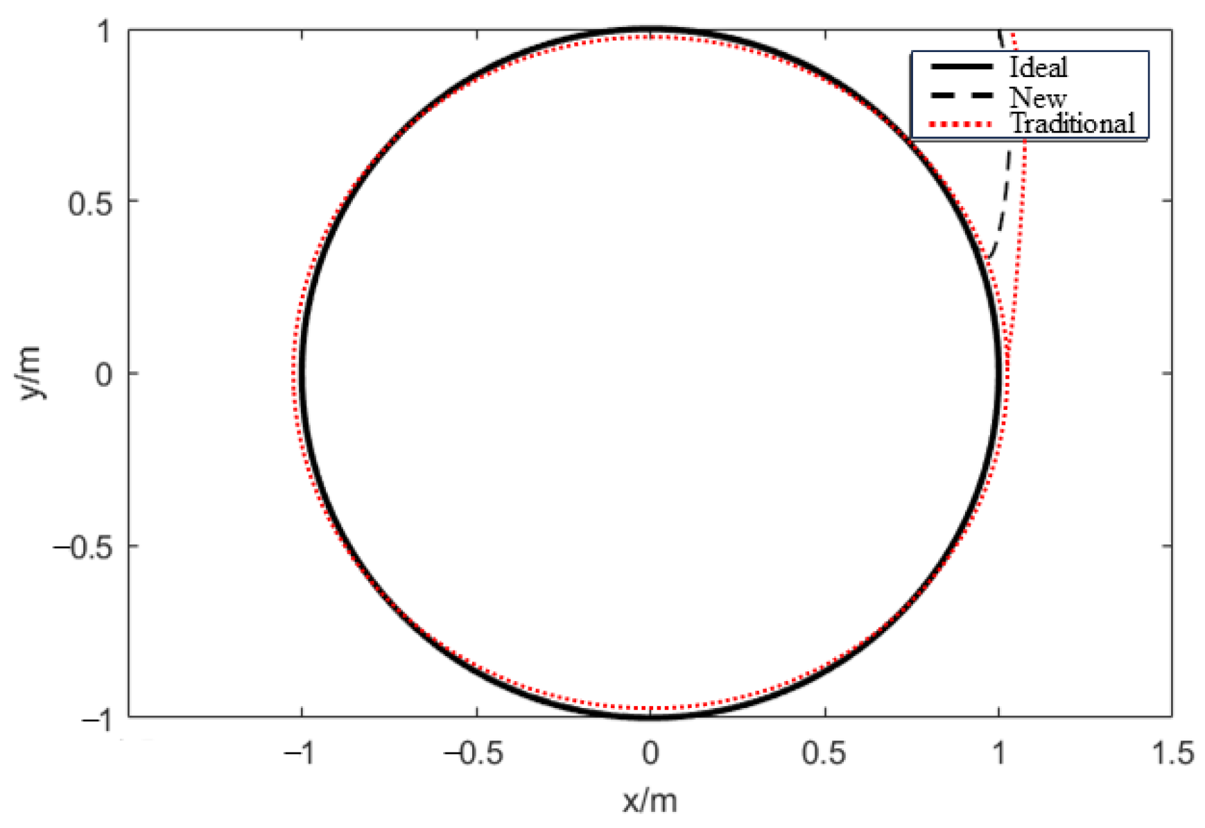
4.1. Simulation Analysis of Mobile Platform

To verify the accurate behavior of the proposed control method, simulation experiments are carried out in this section. The parameters of the ideal motion trajectory of the mobile platform are as follows: $v_d=1.5$, $w_d=1$, $\gamma =0.1$, $d=0.025$, $\widehat{d}=0.06$. The initial pose is $(x_c,y_c,{\theta }_c)=(1,1,\frac{\pi }{3})$, and the expected trajectory is $x_d=\cos (t)$, $y_d=\sin (t)$, ${\theta }_d=t$. In order to verify that the newly designed sliding mode controller can effectively solve the problems of slow tracking speed, large errors, and the flutter of the robot, this section adopts the research method of comparative analysis, respectively, using the sliding mode controller based on the new reaching law and the traditional sliding mode controller without reaching the law to control the robot, and compares and analyzes the experimental results. The error of the new controller is $(x_e,y_e,{\theta }_e)$, and the error of the linear velocity and angular velocity is $v_e$ and ${\omega }_e$. The error of the traditional controller is $(x_u,y_u,{\theta }_u)$, and the error of the linear velocity and angular velocity is $v_u$ and ${\omega }_u$. The system parameters refer to

Table 2. New approach rate parameter.

Parameter	k1	k2	k3	$\mathit{\alpha }$	$\mathit{a}$	$\mathit{b}$
$v$	1	0.8	9	1.5	1.7	0.5
$\omega$	1.1	0.8	9	0.9	1.6	0.5

, and the simulation results are shown in Figure 7, Figure 8, Figure 9 and Figure 10.

As can be seen from Figure 7, the new reaching law proposed in this paper makes the robot’s motion in direction $X$, $Y$, $\theta$ converge within 2 s with a small error, and the closed-loop system tends to be stable immediately. As can be seen from Figure 8, $\widehat{d}$ can converge from 0.06 m to 0.025 m within 1 s. Therefore, the system can still quickly adjust the pose error under the action of the adaptive law when the robot’s centroid distance is unknown. As can be seen from Figure 9, the convergence of $v$ and $\omega$ of the robot can be completed within 1 s. As can be seen from Figure 10, the robot system enters a stable state and has good trajectory tracking performance. Through comprehensive comparative analysis, it can be concluded that the new controller has superior performance and effectively solves the problems of slow robot tracking speed, large errors, and chattering.

4.2. Mobile Platform Trajectory Tracking Experiment

The trajectory tracking test for the mobile platform is conducted to evaluate its performance. This involves navigating the robot along a predefined trajectory to assess its ability to accurately follow the preset path. To better observe the robot’s motion process, we removed the manipulator section and the outer shell of the robot. The length of the preset path (1) is 700 mm, the preset path (2) is 1200 mm, and the robot speed is 700 mm/min. The movement of the robot is depicted in Figure 11.

During the motion process, users only need to set the preset path and choose the robot’s operating speed on the upper computer. The robot then automatically completes trajectory tracking, and it also controls the speed automatically during turns to ensure smooth operation. As shown in Figure 11, the robot essentially meets the functional requirements. The experimental results show that the robot using the new SMC method takes 68.84 s to complete the tracking of the preset path (1), 29.12 s to complete the turning movement, and 102.85 s to complete the tracking of the preset path (2). The time of the robot using the traditional SMC method is 73.56 s, 31.42 s, and 118.39 s, respectively. After analysis, the time of the new SMC method to complete the preset path (1) tracking, turning movement, and preset path (2) tracking is reduced by 12.37%, 7.32%, and 13.13%, respectively, which effectively solves the problems of slow tracking speed, large errors, and the flutter of the mobile platform.

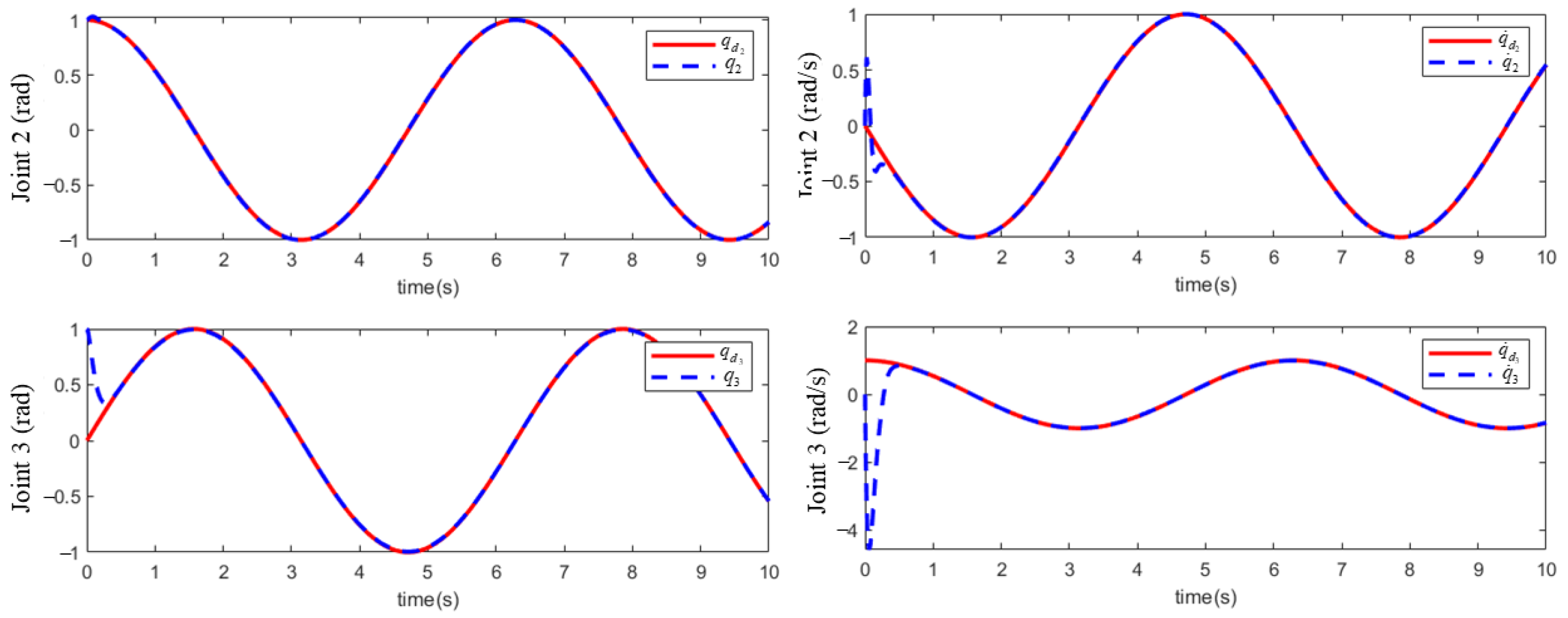
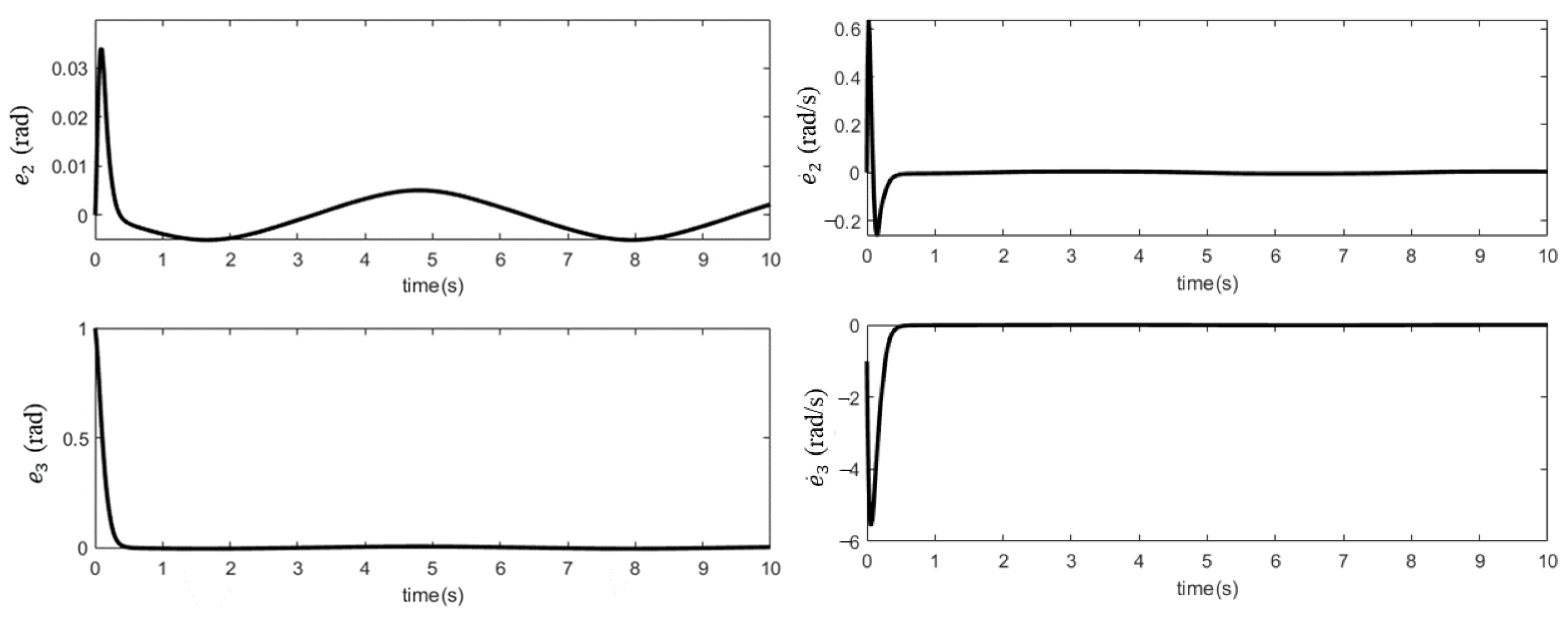
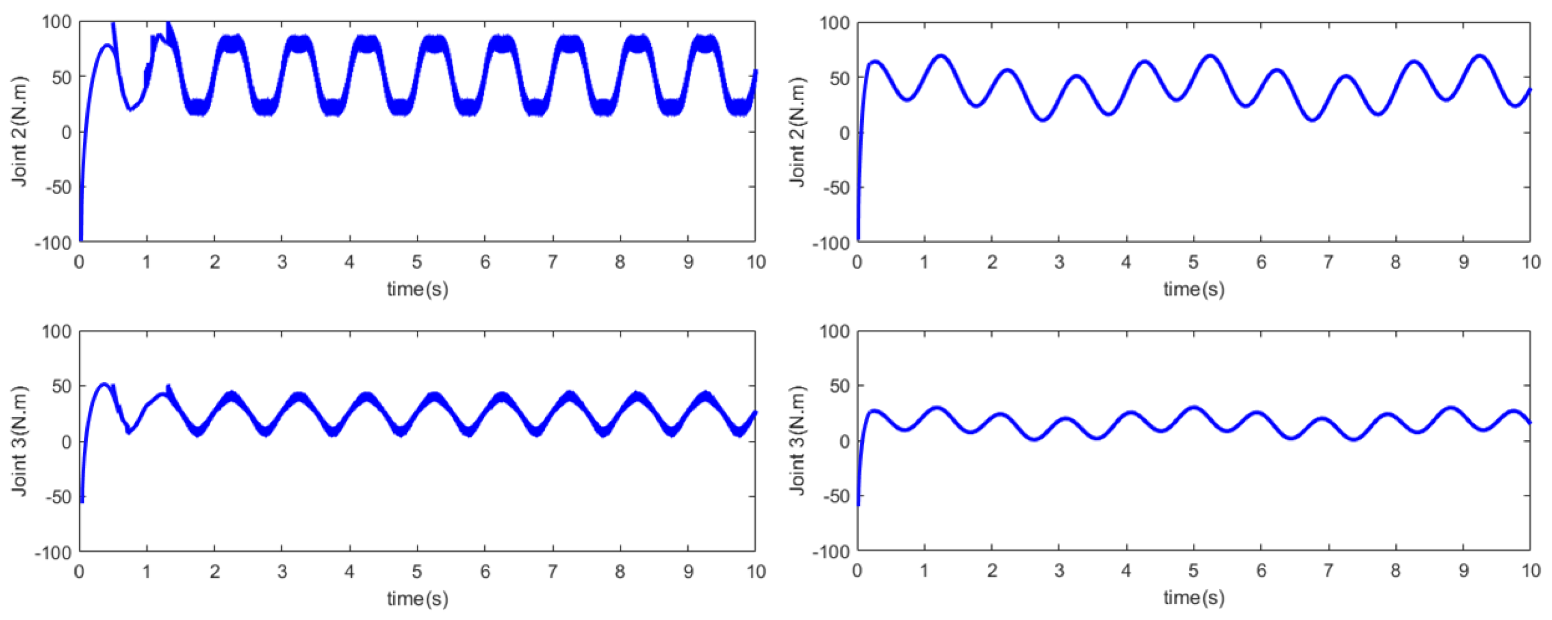
4.3. Simulation Analysis of Manipulator

To facilitate this study, by simplifying the manipulator, the second joint and the third joint were formed into a double-joint manipulator, and the simplified dynamic model of the manipulator was obtained as follows:

$$\begin{array}{c}M\ddot{q}+C\dot{q}+G=\tau +d\\ M\left(q\right)=[\begin{array}{cc}{H}_1+H_2+2H_3\cos q_3& H_2+H_3\cos q_3\\ H_2+H_3\cos q_3& H_2\end{array}]\\ C\left(q,\dot{q}\right)=[\begin{array}{cc}{H}_3{\dot{q}}_3\sin q_3& H_3\left({\dot{q}}_2-{\dot{q}}_3\right)\sin q_3\\ H_3{\dot{q}}_2\sin q_3& 0\end{array}]\\ G\left(q\right)=\left[\begin{array}{c}-H_{4}g\cos q_2-H_{5}g\cos \left(q_2+q_3\right)\\ -H_{5}g\cos \left(q_2+q_3\right)\end{array}\right]\end{array}$$

(30)

where $H_1=\left(m_2+m_3\right)a_2^2$, $H_2=m_3{a}_3^2$, $H_3=m_3{a}_2{a}_3$, $H_4=\left(m_2+m_3\right)a_2$, and $H_5=m_3{a}_3$. The external interference amount is $d(t)=\left[\begin{array}{c}0.1\sin (t);0.1\sin (t)\end{array}\right]$, the expected trajectory of the two joints is $q_d=\left[\begin{array}{c}\cos (t);\sin (t)\end{array}\right]$, and the initial state is $q_0=\left[\begin{array}{c}1;0;1;0\end{array}\right]$. The relevant parameters of the manipulator are $m_2=2.5 \mathrm{kg}$, $m_3=4 \mathrm{kg}$, $a_2=0.23 \mathrm{m}$, $a_3=0.27 \mathrm{m}$, $g=9.8 \mathrm{m}/\mathrm{s}$, and $t=10 \mathrm{s}$.

Table 3. Related parameters of convolutional neural network.

z	H11	H12	H21	H22	M1	M2	rw	rb
5	2	2	1	4	5	5	5	5

shows the relevant parameters of CNN. The simulation results are shown in Figure 12, Figure 13 and Figure 14.

The initial weights $w$ and biases $b$ of the CNN are initialized with random values within the range of [−1, 1]. The controller’s performance can be evaluated by analyzing the states $q_2$, $q_3$, ${\dot{q}}_2$ and ${\dot{q}}_3$. Figure 12 displays the position and velocity tracking curves for joint 2 and joint 3 of the manipulators. The control method proposed in this paper enables the manipulator’s two joints to approach the desired trajectory in the time of 0.5 s, indicating that the controller effectively guides the manipulator to track the required angles. Furthermore, the establishment time for states $q_2$, $q_3$, ${\dot{q}}_2$ and ${\dot{q}}_3$ is finite, signifying that the system reaches a stable state within a reasonable time. This demonstrates the rapid convergence characteristic of the proposed controller.

In Figure 13, the corresponding error signals for the two states are depicted. The error signal represents the difference between the desired trajectory and the actual measured values of the system states. The error signals converge to zero, indicating that the proposed controller successfully minimizes the difference between the desired trajectory and the system states. This affirms the controller’s ability to accurately track the required trajectories, ensuring precise and reliable operation, thereby enhancing the system’s performance and stability.

Figure 14 shows the control signals applied to the two joints of the manipulator after the application of the traditional controller and the new controller, respectively. They were designed to generate the necessary torque or force to drive both joints. As can be seen from the figure, the control signal curve generated by the application of the new controller is smoother, greatly reducing buffeting and accurately tracking the desired trajectory.

5. Conclusions

In this paper, a new and efficient mobile robot is designed to increase the smooth obstacle crossing function without affecting the welding operation. By designing a new SMC, the precise control of the robot is realized, and the problems such as slow tracking speed, large errors and flutter are effectively solved. The stability of the mobile robot control system is proved by the Lyapunov function. Through simulation analysis and testing, it is concluded that the mobile platform can complete convergence within 2 s, and the tracking error is very small. In the simplified manipulator, the variables $q_2$, $q_3$, ${\dot{q}}_2$ and ${\dot{q}}_3$ converge within 0.5 s with errors not exceeding 0.01 m, resulting in smoother control signals and resolving to chatter. In future work, we intend to increase the number of high-precision sensors to achieve remote automated control.

References

1. Seungwoo, H.; Yong, U.; Jaejun, P.; HaeWon, P. Agile and versatile climbing on ferromagnetic surfaces with a quadrupedal robot. Sci. Robot. 2022, 7, eadd1017. [Google Scholar]
2. Yang, P.; Sun, L.; Zhang, M. Design and analysis of a passive adaptive wall-climbing robot on variable curvature ship facades. Appl. Ocean Res. 2024, 143, 103879. [Google Scholar] [CrossRef]
3. Wang, T.; Xue, Z.L.; Dong, X.Q.; Xie, S.L. Autonomous intelligent planning method for welding path of complex ship components. Robotica 2020, 39, 428–437. [Google Scholar] [CrossRef]
4. Feng, X.B.; Tian, W.; Wei, R.; Pan, B.W.; Chen, Y. Application of a wall-climbing, welding robot in ship automatic welding. J. Coast. Res. 2020, 106, 609–613. [Google Scholar] [CrossRef]
5. Jiang, Z.; Zhao, Z.; Chen, B.; Li, Y.C.; Zhao, Y.S.; Xu, Y.D. Design and analysis of a passive adaptive wall-climbing robot based on five-bar mechanisms. Ocean Eng. 2024, 298, 117140. [Google Scholar] [CrossRef]
6. Abdulkader, R.E.; Veerajagadheswar, P.; Lin, N.H.; Kumaran, S.; Vishaal, S.R.; Mohan, R.E. Sparrow: A magnetic climbing robot for autonomous thickness measurement in ship hull maintenance. Mar. Sci. Eng. 2020, 8, 469. [Google Scholar] [CrossRef]
7. Olivier, K. A magnetic climbing robot to perform autonomous welding in the shipbuilding industry. Robot. Comput. Integr. Manuf. 2018, 53, 178–186. [Google Scholar]
8. Ye, D.; Shikun, L.; Xukun, R.; Chaofang, X.; Xinlei, N. Review of key technologies of climbing robots. Front. Mech. Eng. 2023, 18, 4. [Google Scholar]
9. Nagano, K.; Fujimoto, Y. Simplification of motion, generation in the singular, configuration of a wheel-legged, mobile robot. IEEJ J. Ind. Appl. 2019, 8, 745–755. [Google Scholar] [CrossRef]
10. Zhongcheng, G.; Yongjun, D.; Zhongxi, S.; Tangjie, X.; Yonglong, L.; Fan, Z.; Na, D.; Jiandong, W. Design and experimental verification of an intelligent wall-climbing welding robot system. Ind. Robot. 2014, 41, 6–507. [Google Scholar]
11. Lee, D.; Seo, T.; Kim, J.W. Optimal design and workspace analysis of a mobile welding robot with a 3P3R serial manipulator. Robot. Auton. Syst. 2011, 59, 813–826. [Google Scholar] [CrossRef]
12. Andaluz, V.; Roberti, F.; Toibero, J.M. Adaptive unified motion control of mobile manipulators. Control Eng. Pract. 2012, 20, 1337–1352. [Google Scholar] [CrossRef]
13. Yu, C.; Kan, N.; Kawaguchi, T.; Hashimoto, S. Path following for autonomous mobile robots with deep reinforcement learning. Sensors 2024, 24, 561. [Google Scholar] [CrossRef] [PubMed]
14. Zhang, T.; Shi, P.; Li, W.L.; Yue, X.K. Discrete nonsingular terminal sliding mode control for trajectory tracking of space manipulators with mismatched multiple disturbances and noisy measurements. Aerosp. Sci. Technol. 2024, 144, 108766. [Google Scholar] [CrossRef]
15. Hsu, L.; Cunha, V.P.J.; Costa, R.R. Nyquist criterion for chattering avoidance and global stability in observer-based sliding-mode control with parasitics. J. Frankl. Inst. 2024, 361, 106658. [Google Scholar] [CrossRef]
16. Jianing, Z.; Fujie, W.; Guilin, W. Sliding-mode control for teleoperation system with uncertain kinematics and dynamics: An observer-based approach. J. Frankl. Inst. 2023, 360, 8300–8319. [Google Scholar]
17. Wang, S.; Jiang, C.; Tu, Q.; Zhu, C. Sliding mode control with an adaptive switching power reaching law. Sci. Rep. 2023, 13, 16155. [Google Scholar] [CrossRef]
18. Sharaf, A.M.; Armghan, H.; Ali, N. Hybrid control of the DC microgrid using deep neural networks and global terminal sliding mode control with the exponential reaching law. Sensors 2023, 23, 9342. [Google Scholar] [CrossRef]
19. Song, T.Z.; Fang, L.J.; Zang, Y.; Shen, H.S. Recursive terminal sliding mo-de based control of robot manipulators with a novel sliding mode disturbance observer. Nonlinear Dyn. 2023, 112, 1105–1121. [Google Scholar] [CrossRef]
20. Truong, T.N.; Vo, A.T.; Kang, H.J. A novel ANSMC algorithm for tracking control of 3-DOF planar parallel manipulators. Int. J. Mech. Eng. Robot. Res. 2023, 12, 32–39. [Google Scholar] [CrossRef]
21. Vo, T.A.; Truong, N.T.; Kang, J.H. Fixed-Time RBFNN-based prescribed performance control for robot manipulators: Achieving global convergence and control performance improvement. Mathematics 2023, 11, 2307. [Google Scholar] [CrossRef]
22. Yen, T.V.; Nan, Y.W.; Cuong, V.P. Robust adaptive sliding mode neural networks control for industrial robot manipulators. Int. J. Control Autom. Syst. 2019, 17, 783–792. [Google Scholar] [CrossRef]
23. Van, M.; Ge, S.S. Adaptive fuzzy integral sliding-mode control for robust faul tolerant control of robot manipulators with disturbance observer. IEEE Trans. Fuzzy Syst. 2020, 29, 1284–1296. [Google Scholar] [CrossRef]
24. Duan, J.G.; Zhang, H.Z.; Zhang, Q.L.; Qin, J.Y. Research on neural network terminal sliding mode control of robotic arms based on novel reaching law and improved salp swarm algorithm. Actuators 2023, 12, 464. [Google Scholar] [CrossRef]
25. Liu, W.K.; Shu, F.; Xu, Y.L.; Ding, R.Z.; Yang, X.F.; Li, Z.; Liu, Y. Iterative learning based neural network sliding mode control for repetitive tasks: With application to a PMLSM with uncertainties and external disturbances. Mech. Syst. Signal Process. 2022, 172, 108950. [Google Scholar] [CrossRef]
26. Nguyen, T.T.; Tuan, A.V.; Hee-Jun, K. Neural network-based sliding mode controllers applied to robot manipulators: A review. Neurocomputing 2023, 562, 126896. [Google Scholar]
27. Galarza, J.; Oraby, T. Functional data learning using convolutional neural network. Mach. Learn. Sci. Technol. 2024, 5, 015030. [Google Scholar] [CrossRef]
28. Dai, Y.W.; Wu, Q.B.; Zhang, Y. Generalized sparse radial basis function networks for multi-classification problems. Appl. Soft Comput. 2024, 154, 111361. [Google Scholar] [CrossRef]
29. Ying, K.; Yunliang, J.; Junwen, Z.; Huifeng, W. A time controlling neural network for time-varying QP solving with application to kinematics of mobile manipulators. Int. J. Intell. Syst. 2020, 36, 403–420. [Google Scholar]
30. Bo, T.; Xingwei, Z.; Sijie, Y.; Han, D. Kinematic modeling and control of mobile robot for large-scale workpiece machining. Proc. Inst. Mech. Eng. Part B J. Eng. Manuf. 2020, 236, 29–38. [Google Scholar]
31. Panahandeh, P.; Alipour, K.; Tarvirdizadeh, B.; Hadi, A. A kinematic Lyapunov-based controller to posture stabilization of wheeled mobile robots. Mech. Syst. Signal Process. 2019, 134, 106319. [Google Scholar] [CrossRef]
32. Xu, Z.Z.; Cao, G.Z.; Huang, S.D.; Zheng, H.X. Sliding mode control of the planar switched reluctance motor for interference suppression. ICIEA 2016, 11, 2130–2134. [Google Scholar]
33. Li, Z.; Ren, J. Adaptive event-triggered non-fragile sliding mode control for uncertain T-S fuzzy singular systems with passive constraint. Appl. Math. Comput. 2024, 472, 128629. [Google Scholar] [CrossRef]
34. Chen, J.Q.; Zhang, H.Y.; Zhu, T.T.; Pan, S.T. Trajectory tracking control of a manipulator based on an immune algorithm-optimized neural network in the presence of unknown backlash-like hysteresis. Appl. Math. Comput. 2024, 470, 128552. [Google Scholar] [CrossRef]
35. Ma, H.F.; Wu, J.F.; Xiong, Z.H. A Novel Exponential Reaching Law of Discrete-Time Sliding-Mode Control. IEEE Trans. Ind. Electron. 2017, 64, 3840–3850. [Google Scholar] [CrossRef]
36. Yang, X.H.; Zhao, Z.Y.; Li, Y.T.; Yang, G.C.; Zhao, G.D.; Liu, H. Adaptive neural network control of manipulators with uncertain kinematics and dynamics. Eng. Appl. Artif. Intell. 2024, 133, 107935. [Google Scholar] [CrossRef]
37. Hamed, N.R.; Abolfazl, Z.; Holger, V. Actor–critic learning based PID control for robotic manipulators. Appl. Soft Comput. 2024, 151, 111153. [Google Scholar]
38. Zhou, M.H.; Feng, Y.; Xue, C.; Han, F.L. Deep convolutional neural network based fractional-order terminal sliding-mode control for robotic manipulators. Neurocomputing 2020, 416, 143–151. [Google Scholar] [CrossRef]
Figure 1. Mechanical structure of mobile manipulator.
Processes 12 00881 g001
Figure 2. Robot obstacle crossing diagram.
Processes 12 00881 g002
Figure 3. The principle of differential steering.
Processes 12 00881 g003
Figure 4. Six-wheel mobile platform and equivalent model diagram.
Processes 12 00881 g004
Figure 5. Convolutional neural network model.
Processes 12 00881 g005
Figure 6. Structure diagram of control system.
Processes 12 00881 g006
Figure 7. Trajectory error convergence.
Processes 12 00881 g007
Figure 8. Center of mass distance convergence.
Processes 12 00881 g008
Figure 9. Velocity error convergence.
Processes 12 00881 g009
Figure 10. Trajectory tracking.
Processes 12 00881 g010
Figure 11. Mobile platform trajectory tracking test.
Processes 12 00881 g011
Figure 12. Position and velocity tracking.
Processes 12 00881 g012
Figure 13. Tracking error.
Processes 12 00881 g013
Figure 14. Trajectories of control input.
Processes 12 00881 g014