Oil–Water Hydrodynamics Model during Oil Displacement by Water in Down-Hill Mobile Pipeline

Abstract

In the process of water displacing oil within mobile pipelines, it is common that the oil tends to accumulate at the elevated sections of inclined pipelines, leading to an issue of residual oil accumulation. In this paper, the mechanism of carrying accumulated oil out of the pipeline with water flow is discussed. Taking the residual oil layer in down-hill pipelines as a research object, a hydrodynamic model of the water-oil displacement process is established based on the theory of liquid–liquid two-phase flow and the application of the momentum transfer equation. It has been found that the use of this model can enhance the computational speed by 15% without affecting the accuracy of the calculations. Subsequently, the model is used to analyze the impact of different initial water-phase velocities, inclination angles, initial oil-phase heights, and pipeline diameters on the oil-carrying process of water flow. The results indicate that increasing the initial water-phase velocity, the angle of inclination, and the initial oil-phase height all enhance the fluctuation in the oil–water interface, making it easier for the oil phase to be carried away from the pipeline. Conversely, when all other parameters are held constant, an increase in the pipeline diameter tends to stabilize the oil–water interface, thereby making it more difficult for the residual oil to be carried away by the water flow.

1. Introduction

A mobile pipeline is an assembly-type system that can be laid out and retrieved on an immediate basis, and belongs to a category of fuel transportation equipment, whose primary function is to transport fuel from the strategic and tactical rear-to-forward mobile fuel depots, fuel stations, and combat troops. Typically, this system consists of pipes, mobile oil pumps, valves, measuring instruments, etc., and is connected through detachable joints (either socket-type or flanged-type). During combat and military training exercises, it is laid directly on the surface of the ground, and is characterized by its rapid deployment and retrieval, as well as its flexibility and mobility [1]. In contrast to fixed pipelines, mobile pipelines must be retrieved after completing the oil transport mission, and then quickly repositioned in other areas for the next oil transport operation. Therefore, the retrieval speed of the mobile pipeline directly affects the efficiency of pipeline oil transportation support. Before the retrieval or maintenance of the mobile pipelines, the fuel inside must be drained and then recovered into oil tanks or fuel trucks. Currently, pipeline emptying operations mainly adopt three methods: free-flow drainage, gas displacement, and water displacement. The water displacement method employs oil pumps to directly inject water, and gradually displace the fuel from the pipelines. Compared to free-flow drainage and gas displacement, the water displacement method exhibits several advantages including lower terrain requirements, direct utilization of oil transportation equipment, a simple process, a fast speed, minimal loss of oil and gas, and high safety. It is therefore widely used. For example, when the temperature and water source conditions permit, the water displacement method is preferred [2].

During the water displacement process, the oil phase and water phase are immiscible, and there is a density difference and polarity difference between the two, making it difficult to form a stable emulsion [3]. Due to the lower density of oil, the oil in the pipeline tends to gather at the high sections of the pipelines because of its buoyancy, resulting in residual oil formation, which is challenging to be displaced by water flow. This increases the difficulty of the water displacement process, but also leads to lower efficiency in the mobile pipeline displacement. After multiple practical water displacement operations, it has been found that residual oil is highly likely to accumulate in down-hill pipelines. If the residual oil is not cleaned up, the wastewater directly discharged into the ground or rivers, lakes, and reservoirs will inevitably cause environmental pollution. To avoid pollution, it is necessary to add oil-mix-receiving and treatment devices at the end of the pipeline, which in turn increases the difficulty of pipeline laying. Therefore, there is an urgent need to study the mechanism of oil-carrying of water flow in the water displacing oil process in down-hill pipelines. This could improve the efficiency of water displacement operations, reduce retrieval time, and enhance the effectiveness of the pipeline oil transportation support. In addition, it improves the current pipeline displacement theories and thoughts on pipeline design, which has very important engineering significance and practical value.

At present, the research on the flow characteristic of water displacing oil in mobile pipelines mainly focuses on the oil–water mixed model [4,5,6,7] and mixed oil cutting technology [8,9]. Zhang et al. [6] established an oil–water mixing model during the emptying process in a mobile pipeline based on the theory of the sequential transmission of refined oil products and two-dimensional convection diffusion, and taking into account the interaction between convection and turbulence. Zhang et al. [7] established an oil mixing model of sequential transportation of gasoline and water, and simulated it with the computational fluid dynamics software PHEONICS (latest v. 2023). Through a comparison with the sequential transportation of gasoline–diesel, the special oil mixing change law of the sequential transportation of gasoline–water was analyzed. Based on the results of the indoor loop experiment of the water-carrying of oil flow in a relief pipeline, the distribution form of water in oil-carrying water, the critical condition of water carried by oil flow, and the main parameters affecting the critical condition were analyzed [10]. Zhang et al. [11] established an oil–water velocity model during oil-carrying water movement in up-dip pipeline based on the theory of the two-phase stratified flow of oil and water, and analyzed the effects of oil velocity, pipeline up-dip angle, pipe diameter, and water-phase thickness on the proportion of water-phase reflux.

Liquid–liquid displacement flow has a wide range of industrial applications, including emptying flow by water displacing oil in mobile pipelines. Taghavi et al. [12,13] studied the flow law of high-density salt water displacement of low-density clear water in pipelines under different dip angles through experiments. According to the difference in dominant stress in the flow process, the flow was divided into five flow patterns, and it was observed that a retention layer remains in the pipeline under low flow velocity. Caliman et al. [14] found through experiments that in the liquid–liquid displacement flow dominated by buoyancy, the pipeline inclination angle has a great influence on the flow pattern. Hasnain et al. [15,16] established a flow characteristic model of the displaced liquid based on the change law of the cross-sectional area and height of the displaced liquid in the liquid–liquid displacement flow over time, and obtained the relationship between the front velocity and the inlet velocity of the displaced fluid. Oladosu et al. [17] studied the differences in displacing flows between heterogeneous solutions, and found that displacing flows between heterogeneous solutions with a high Peclet number (Pe) showed similar flow characteristics. Chattopadhyay et al. [18,19,20,21] simulated the displacement flow of liquids with different densities driven by pressure. In the initial stage of displacement, the displacement rate was significant, and the volume fraction of the displaced liquid dropped rapidly. After a period of time, the displacement rate tended to be stable. The water-combined transport mode adopted in the fixed pipeline is essentially the flow process of oil displacing water, and the replacement between oil and water is accomplished by injecting diesel oil into the first station. Li [22] and Wang et al. [23] designed a physical model for predicting the location and distance of the dissatisfied flow in the pipeline and the volume fraction concentration of the oil–water mixture based on the sequential transport theory, aiming at the whole process of water-combined transport in a fixed pipeline with a large drop.

The current research on the mechanisms of water displacing oil primarily revolves around the oil–water mixture models for fixed pipelines and the displacement flow characteristics between immiscible liquids. A research gap remains in relation to the water displacement of oil flow characteristics in the down-hill sections of mobile pipelines. To investigate the mechanism of water displacing oil flow, this paper, based on the theory of liquid–liquid two-phase flow, establishes a hydrodynamic model for the water displacing oil process in the down-hill sections of mobile pipelines, and analyzes the impact of different initial water-phase velocities, dip angles, initial oil-phase thickness, and pipeline diameters on flow characteristics, providing recommendations for improving the displacement efficiency in mobile pipelines accordingly.

2. Mathematical Model

During the process of water displacing oil, the residual oil within the pipeline will enter the down-dip pipeline under the action of the water phase. Due to the change in the direction of gravity relative to the pipeline wall, the oil phase will float upwards. When the shear stress between the water–oil phase is less than the component of the buoyant force of the oil phase in the axial direction of the pipeline, the oil phase will accumulate at the upper part of the pipeline, and the accumulated oil phase in the pipeline will be in a slanted and relatively stationary state.

2.1. Two-Dimensional Liquid Layer Model

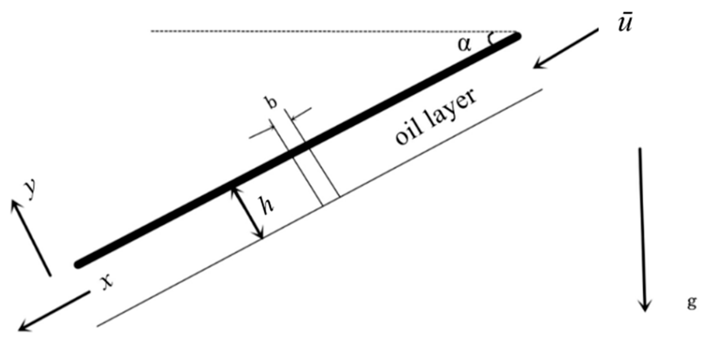
In mobile pipelines, there are joints and other recesses inside, but compared to the entire pipeline, the impact on the oil–water interface is relatively small. Therefore, it is assumed that the inner wall of the pipeline is smooth for the sake of convenience in the calculation. To study its motion, a two-dimensional cross-section is taken for analysis, and the geometric model is shown in Figure 1.

As is shown in Figure 1, there exists a residual oil layer with a certain thickness on the upper side of the down-dip straight circular pipe. Taking this oil layer as the research object, a geometric model is established considering the gravity, buoyancy, shear stress between the oil phase and the pipe wall, and the shear stress at the interface between the oil and water phases. Since the thickness of the oil layer is relatively small, compared to the pipe diameter, it can be considered as if the oil layer is spread on an inclined plane with an angle α. The average width of the oil layer is $l=\frac{D}{2}\beta$. Let the simplified cross-sectional area of the residual oil layer be equal to the cross-sectional area of the residual oil layer in the circular pipe, that is,

$$\frac{D}{2}\beta h=\frac{D^2}{8}(\beta -\sin \beta )$$

(1)

where D represents the diameter of the cross-section of the inclined circular pipe; h denotes the thickness of the residual oil layer on the upper side of the pipeline; and β corresponds to the central angle of the residual oil layer. Therefore, it can be concluded that

$$h=\frac{D}{4}(1-\frac{\sin \beta }{\beta })$$

(2)

The water-phase momentum conservation equation is established in the x direction by considering the microelement segment with axial length dx in the pipeline

$$\left[{\rho }_w\mathrm{gsin}\alpha -\frac{\mathrm{d}p}{\mathrm{d}x}\right]\mathrm{d}x\pi \frac{D^2}{4}={\tau }_{\mathrm{i}}\frac{D}{2}\beta \mathrm{d}x+{\tau }_w\left(2\pi -\beta \right)\frac{D}{2}\mathrm{d}x$$

(3)

where ρ_w represents the density of water; g stands for the acceleration due to gravity; α denotes the angle of inclination of the pipeline; p is the pressure at the cross-section x; D is the diameter of the cross-section of the inclined circular pipe; τ_i is the shear stress at the oil–water interface; and τ_w is the shear stress between the water phase and the pipeline wall. Therefore, the pressure gradient along the x-direction can be derived as follows:

$$-\frac{\mathrm{d}p}{\mathrm{d}x}={\tau }_i\frac{2\beta }{\pi D}+{\tau }_w\frac{2}{D}\left(2-\frac{\beta }{\pi }\right)-{\rho }_{w}g\sin \alpha$$

(4)

2.2. Calculation of Shear Stress

The theory of oil–water two-phase flow provides an empirical formula for interfacial shear stress [24,25,26,27], which includes the empirical formula for shear stress between the liquid and the wall, as well as the shear stress between the oil–water two-phase interface. The shear stress between the oil–water interface can be determined by the following formula:

$${\tau }_i=\frac{1}{2}{\lambda }_w{\rho }_w{\left(u_w-\overline{u}\right)}^2$$

(5)

$$\overline{u}=Q/h$$

(6)

where τ_i represents the shear stress at the oil–water interface; λ_w is the friction factor for the water flow; ρ_w is the density of the water phase; u_w is the velocity of the water flow; $\overline{u}$ is the average velocity of the oil phase; Q is the flow rate of the oil phase; and h is the thickness of the oil phase.

The shear stress between the water phase and the wall can be calculated using the following empirical formula:

$${\tau }_w=\frac{1}{2}{\lambda }_w{\rho }_w{u_w}^2,{\lambda }_w=\{\begin{array}{c}16{\mathrm{Re}}^{-1}\\ 0.046{\mathrm{Re}}^{-0.2}\end{array}\begin{array}{c}\\ \end{array}\begin{array}{c}\mathrm{Re}\le 1500\\ \mathrm{Re}>1500\end{array}\begin{array}{c}\\ \end{array},\mathrm{Re}=\frac{{\rho }_w{u}_{w}D}{{\mu }_w}$$

(7)

where τ_w represents the shear stress between the water phase and the wall; Re is the Reynolds number of the water flow; and μ_w is the dynamic viscosity of the liquid water. By combining Equations (5)–(7), the following results can be obtained:

$${\tau }_i=\{\begin{array}{c}8{\mathrm{Re}}^{-1}{\rho }_w{\left(u_w-\frac{Q}{h}\right)}^2\\ 0.023{\mathrm{Re}}^{-0.2}{\rho }_w{\left(u_w-\frac{Q}{h}\right)}^2\end{array}\begin{array}{c}\\ \end{array}\begin{array}{c}\begin{array}{l}\mathrm{Re}\le 1500\\ \end{array}\\ \mathrm{Re}>1500\end{array}$$

(8)

From the above formula, it is apparent that the shear stress between the oil–water phase is related to parameters such as the Reynolds number of the water flow, the density of the water phase, the thickness of the residual oil layer, and the velocity difference between the two phases, among which the velocity difference between the oil and water phases has the greatest influence on the change in shear stress.

2.3. Oil-Phase Flow Momentum Transfer Equation

According to the coordinate system in Figure 2, the retained oil layer in the circular pipe is still simplified as being spread flat on an inclined plane. A small control volume with a thickness of b is taken for analysis. Based on the Lagrange rule and considering the conservation of oil-phase mass and momentum, it is assumed that the thickness of the oil layer h varies with the position in the x direction. Therefore, the volumetric flow rate of the oil layer per unit width is:

$$Q={\displaystyle {\int }_0^h{u}_{o}dy}$$

(9)

where u_o represents the velocity of the oil phase. According to the principles of mass conservation and momentum conservation, one can derive the following:

$$\frac{dQ}{dt}=\frac{dh}{dt}{u}_{\mathrm{i}}+{\displaystyle {\int }_0^h\frac{du}{dt}dy}=0$$

(10)

$$\rho \frac{d}{dt}\left({\displaystyle {\int }_0^h{u}_{o}bdy}\right)=\left({\tau }_i-{\tau }_o\right)b-{\rho }_{0}ghb\sin \alpha -h\frac{dp}{dx}b$$

(11)

where u_i is the interface velocity; ρ_o is the density of the oil phase; and τ_o is the shear stress between the oil layer and the wall. Substituting Equation (4) into Equation (11), the left side of the equation can be further obtained as follows:

$$\frac{d}{dt}{\displaystyle {\int }_0^h{u}_{o}bdy}=-\frac{dh}{dt}{u}_{\mathrm{i}}b$$

(12)

Assuming that other physical quantities do not change with time, one can further obtain the variation in the residual oil layer height with time:

$$\frac{dh}{dt}=-\frac{{\tau }_i}{{\rho }_o{u}_{\mathrm{i}}}\left(1+\frac{2\beta h}{\pi D}\right)+\frac{{\tau }_o}{{\rho }_o{u}_{\mathrm{i}}}-\frac{{\tau }_w}{{\rho }_o{u}_{\mathrm{i}}}\frac{2h}{D}\left(2-\frac{\beta }{\pi }\right)+\frac{gh}{u_{\mathrm{i}}}\sin \alpha \left(1+\frac{{\rho }_w}{{\rho }_o}\right)$$

(13)

Through analyzing the above equation, it reveals that the change in the oil layer height over time is related to the shear stress between the oil phase and the wall, the shear stress between the water phase and the wall, as well as the shear stress between the oil and water phases. In addition, the interface velocity, pipe diameter, pipeline dip angle, and oil density are all main parameters in this model for evaluating the water displacing oil process. Therefore, analyzing the detailed impact of each factor on the oil layer height based on this model can provide a scientific basis for actual water displacing oil operations, thereby optimizing the process of mobile pipeline displacing operations.

2.4. The Setting of Numerical Simulation Parameters

A 3D pipeline model can more truly and accurately reflect the flow state compared to a 2D pipeline model, so this paper selected a 3D pipeline model for simulation, with a pipe diameter of 15 mm and 20 mm. To eliminate the influence of the inlet stress and to ensure that the entire evacuation process is fully developed, the length of the horizontal pipe section is usually not less than 20 times the pipe diameter in the research of the flow characteristics in the down-dip pipe section. Consequently, a length of 0.5 m for the horizontal pipe section and 1 m for the down-dip pipe section were chosen; the curvature radius at the bend R was greater than or equal to 5D, with a curvature radius of 100 mm being taken. The dip angles were 5°, 15°, 30°, and 45°, and the initial oil-phase heights were 2.5 mm, 5 mm, and 7.5 mm. The model was established using the three-dimensional modeling software SolidWorks 2022. Figure 3 shows a three-dimensional pipeline model established for a simulated pipe section with a diameter of 20 mm and a dip angle of 15° for instance.

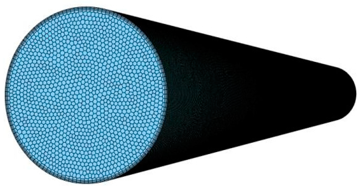
The model employs polyhedral mesh division. Since the oil layer is always positioned on the upper wall of the pipeline, the model is processed by mesh refinement near the wall. Through the analysis of the calculation results, the model established in this paper has improved the calculation speed by 15% compared to the previous oil–water flow model [2,4]. The divided cross-sectional mesh is shown in Figure 4.

3. Results and Discussion

3.1. Classification of Oil–Water Interface during Flow

Due to the differences in parameters such as water-phase velocity, pipe diameter, and dip angle, the oil–water interface will display varying flow patterns. As shown in Figure 5, the oil–water interface can be divided into four types: a smooth interface, a wavy interface, and two types of unstable interfaces. A smooth interface generally appears under conditions with a small water-phase velocity and dip angle, where the oil–water interface is relatively flat and smooth along the pipeline axis. When the flow velocity increases, the oil–water interface begins to fluctuate, but the oil phase is still relatively stationary and not dispersed by the water flow at this time. When the water-phase velocity continues to increase, the oil–water interface produces more violent fluctuations, the oil phase begins to lose stability and produce oil droplets that are carried away by the water phase, and at this time, the oil phase may break; this type of oil–water interface is transient, and the state of the oil phase will also change over time.

Equation (13) shows that the initial water-phase velocity, dip angle, initial oil-phase height, and pipe diameter all directly affect the thickness of the residual oil layer on the upper side of the pipeline during the oil-carrying process of water flow in the inclined pipeline. Therefore, this paper mainly focuses on these parameters and then conducts research, analyzing how these types of factors affect the water-assisted oil drainage process.

3.2. Effect of Initial Water-Phase Velocity on Oil–Water Two-Phase Distribution Pattern

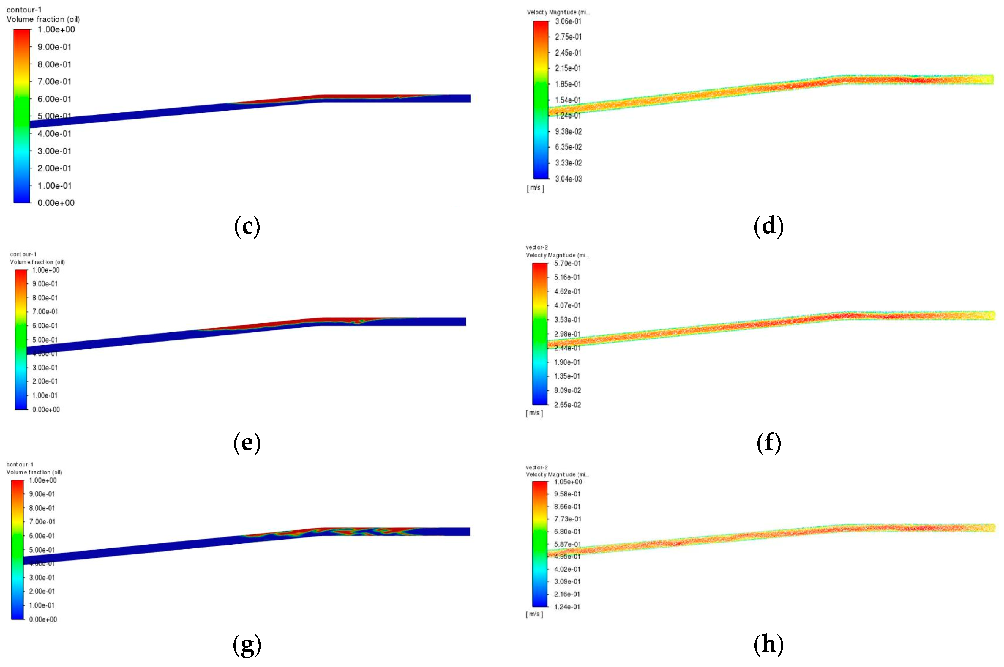
Taking a pipe diameter of 15 mm, a dip angle of 5°, and an initial oil-phase height of 7.5 mm as an example, Figure 6 shows the oil–water distribution patterns and velocity vectors under the conditions of water-phase velocities of 0.1 m/s, 0.2 m/s, 0.4 m/s, and 0.8 m/s, respectively.

From Figure 6a,c,e,g, it can be found that the oil phase gradually moves from the horizontal pipe section to the down-dip pipe section along with the water phase, under the action of shear force. In the meantime, its thickness gradually reduces after the oil layer enters the down-dip section. Under low flow velocities, the oil–water two-phase flow exhibits a distinct, smooth stratified flow pattern; however, as the flow velocity increases, the disturbance at the oil–water interface intensifies, and the interface begins to fluctuate, causing the oil–water two-phase flow pattern to gradually transition from a smooth stratified flow to a wavy stratified flow. When the flow velocity continues to increase and the interface disturbance reaches a certain level, the oil phase begins to detach and disperse into the water phase, eventually resulting in an intermittent flow.

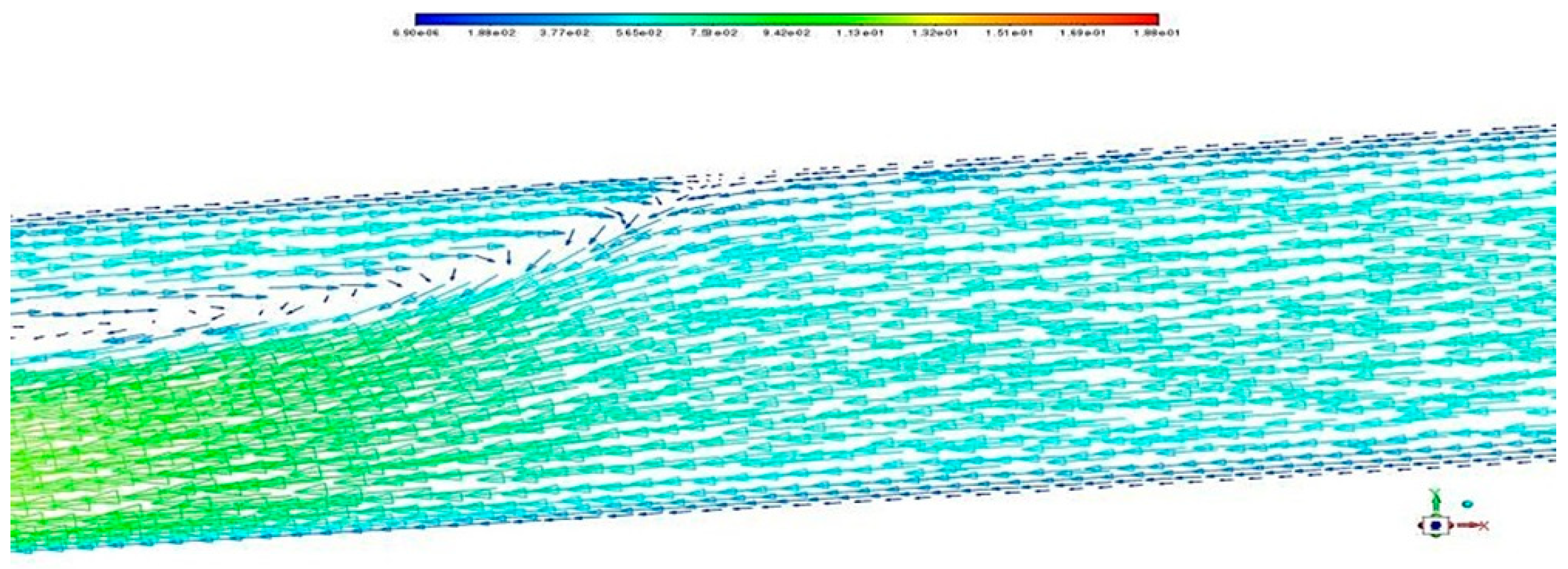
From Figure 6b,d,f,h, it can be observed that the oil–water interface velocities along the axial direction of the pipelines are all positive, and the velocity vectors show that the maximum flow velocity occurs at the lower part of the oil–water interface. The velocity of the oil phase near the wall decreases significantly and under conditions of low water-phase velocity, an oil-phase backflow occurs near the wall, as shown in Figure 7. Therefore, it can be considered that under the action of the oil-phase backflow, the cross-sectional oil-phase content increases, and accordingly, the area occupied by the water phase decreases, the velocity rises, and the shear force increases, thus forming vortices. The corresponding velocity vectors show that the wave peaks coincide with the positions where vortices are generated. The change in flow patterns during the two-phase flow of water carrying oil is caused by the disturbance and destabilization of the oil–water interface, rather than being due to the increase in kinetic energy of the continuous phase as in the traditional oil–water two-phase flows.

In summary, it can be concluded that the fundamental reason the oil phase cannot be carried away from the pipeline by the water flow is the backflow effect of the oil phase. When the carrying action of the water phase on the oil phase is greater than the backflow effect of the oil phase, the oil phase can be carried away from the pipeline, thus preventing the further accumulation of the residual oil.

3.3. Effect of Pipe Dip Angle on Oil–Water Two-Phase Distribution Pattern

Taking the pipe diameter of 15 mm, the water-phase flow rate of 0.4 m/s, and the initial oil-phase height of 7.5 mm as an example, Figure 8 shows the oil–water distribution patterns and velocity vectors under the conditions of dip angle α of 5°, 15°, 30°, and 45°, respectively.

From the figures above, it can be observed that as the dip angle increases, the water-phase velocity magnitude in the down-dip pipeline becomes higher, and the shear force also increases accordingly. The fluctuations at the oil–water interface become more intense, and the oil phase even begins to break at a dip angle of 30°, transitioning from a stratified flow to a wavy flow pattern. When the dip angle reaches 45°, the oil phase starts to become discontinuous. Additionally, from the velocity vectors, it can be found that as the angle increases, the backflow effect becomes more pronounced, with a decrease in velocity magnitude at the location ahead of the oil-phase front, causing severe oil-phase accumulation. The shape of the oil-phase front also transitions from a sharp wedge to a rounded wedge.

3.4. Effect of Initial Oil-Phase Height on Oil–Water Two-Phase Distribution Pattern

The simulations were conducted with a pipe diameter of 15 mm, a dip angle of 15°, and an initial water-phase velocity of 0.4 m/s, respectively. The oil–water distribution patterns and velocity vectors for initial oil-phase heights h of 2.5 mm, 5 mm, and 7.5 mm are depicted in Figure 9.

From Figure 9a,c,e, it can be found that as the initial oil-phase height increases, the shape of the oil-phase front remains unchanged, and the oil–water interface gradually transitions from a smooth interface to an unstable interface. From Figure 9b,d,f, it is shown that the intensification in interface fluctuations is due to the increase in the cross-sectional area occupied by the oil phase as the oil-phase height increases, resulting in a decrease in the area through which the water phase flows. Consequently, an increase in the water-phase velocity to an increase in the interaction forces between the oil and water phases, enhancing the severity of the fluctuations. As a result, it can be considered that, with other conditions held constant, an increase in the initial oil-phase height will promote the transition of the oil–water two-phase distribution from a stable state to an unstable state.

3.5. Effect of Pipe Diameter on Oil–Water Two-Phase Distribution Pattern

The simulations were conducted using pipelines with diameters of 15 mm and 20 mm, both with a dip angle of 15° and an initial water-phase velocity of 0.1 m/s. To ensure that the initial liquid content ratio is consistent for both pipe diameters, the initial oil-phase height is set to 7.5 mm for the 15 mm diameter pipeline and 10 mm for the 20 mm diameter pipeline. Figure 10 shows the oil-phase volume fraction contours and velocity vectors for the two different pipe diameters at 0.5 s. Comparing Figure 10a,c, it can be observed that after the increase in pipe diameter, the fluctuation in the oil–water interface is reduced, and the interface transitions from a wavy interface to a smooth interface. Through analyzing Figure 10b,d, it reveals that, with other parameters held constant according to similar principles, as the pipe diameter increases, the area occupied by the water phase in the cross-section increases, leading to a decrease in the water-phase velocity magnitude through the oil–water interface. Moreover, the shear force reduces, thus making the oil–water interface more stable.

Therefore, it can be concluded that, as the pipe diameter increases, the distribution pattern of the oil–water two-phase system becomes more stable, with other parameters held constant.

All in all, when applying water displacing oil in practical mobile pipeline emptying operations, for down-dip pipelines, methods such as increasing the initial water-phase velocity, enlarging the dip angle, and raising the oil-phase height can be adopted to improve the pipeline emptying efficiency. At the same time, when the flow rate can meet the oil transportation requirements, pipelines with smaller diameters can be used for oil transportation, which can enhance the pipeline emptying efficiency.

4. Conclusions

Based on the analysis of the water flow carrying oil in the inclined pipelines and the theory of liquid–liquid two-phase flow, a hydrodynamic model of oil and water is established. This model takes the residual oil in the upper part of the inclined pipeline as the research object, and comprehensively considers factors such as gravity, buoyancy, shear stress, and momentum transfer of the oil-phase flow, thereby deriving the relationship between the thickness of the residual oil layer in the inclined pipeline and factors such as shear stress, interface velocity, pipeline inclination angle, oil density, and pipe diameter. This paper analyzes the changes in the residual oil layer in the water displacing oil process in the inclined pipeline under five initial water-phase velocities of 0.05 m/s, 0.1 m/s, 0.2 m/s, 0.4 m/s, and 0.8 m/s, four dip angles of 5°, 15°, 30°, and 45°, three retained oil layer thicknesses of 2.5 mm, 5 mm, and 7.5 mm, and two pipeline diameters of 15 mm and 20 mm, respectively.

It is found that the fundamental reason the oil phase is difficult to be carried away by the water flow is the backflow effect of the oil phase. When the carrying action of the water phase on the oil phase is greater than the backflow effect of the oil phase, the oil phase can be carried away from the pipeline, thus preventing the formation of residual oil. Moreover, increasing the initial water-phase velocity, dip angle, and initial oil-phase height will increase the fluctuation degree of the oil–water interface, leading to a transition from stratified flow to dispersed flow in the oil–water two-phase flow, making it easier for the residual oil to be carried away by the water flow. On the other hand, with all other parameters held constant, increasing the pipeline diameter will keep the oil–water flow pattern more stable, making it difficult for the residual oil to be carried away by the water flow.