Artificial Intelligence for Hybrid Modeling in Fluid Catalytic Cracking (FCC)

Abstract

This study reports a novel hybrid model for the prediction of six critical process variables of importance in an industrial-scale FCC (fluid catalytic cracking) riser reactor: vacuum gas oil (VGO) conversion, outlet riser temperature, light cycle oil (LCO), gasoline, light gases, and coke yields. The proposed model is developed via the integration of a computational particle-fluid dynamics (CPFD) methodology with artificial intelligence (AI). The adopted methodology solves the first principle model (FPM) equations numerically using the CPFD Barracuda Virtual Reactor 22.0^® software. Based on 216 of these CPFD simulations, the performance of an industrial-scale FCC riser reactor unit was assessed using VGO catalytic cracking kinetics developed at CREC-UWO. The dataset obtained with CPFD is employed for the training and testing of a machine learning (ML) algorithm. This algorithm is based on a multiple output feedforward neural network (FNN) selected to allow one to establish correlations between the riser reactor feeding conditions and its outcoming parameters, with a 0.83 averaged regression coefficient and an overall RMSE of 1.93 being obtained. This research underscores the value of integrating CPFD simulations with ML to optimize industrial processes and enhance their predictive accuracy, offering significant advancements in FCC riser reactor unit operations.

1. Introduction

Over the past decades, the oil refining industry has faced a convergence of challenges, including a surge in demand for refinery products, a decline in crude oil quality, as well as stricter product quality and environmental constraints. To address these challenges, refineries have invested substantially in research and development (R&D), particularly in the areas of simulation and modeling [1]. One of the focal points of this research has been the fluid catalytic cracking (FCC) process, which has stood out as one of the most extensively studied processes in the modern oil refinery sector. In this regard, it is noteworthy to mention that approximately 45% of the fuel generated in refineries originates from the FCC process and its auxiliary units [2]. Consequently, FCC has evolved into one of the most profitable processes in oil refineries but also one of the most important reactor units in modern industry. Figure 1 describes the key positioning of the FCC reactor as a central unit in the refinery network, where a gas oil feedstock can be converted into fuel gas, gasoline, and heating oil.

The FCC process encompasses three operational stages: (a) the reaction, (b) the product separation, and (c) the catalyst regeneration. During these stages, crude or heavy gas oil undergoes a conversion into a range of lighter chemical species (C₁–C₄), as well as into more valuable compounds like gasoline (C₅⁺–C₁₂) and diesel/cycle oil (C₁₂–C₁₆) [3,4]. The reaction stage takes place under conditions close to atmospheric pressure and within a temperature range of approximately 500–570 °C along the riser reactor unit. In the riser reactor, heavy gas oil is continuously fed and cracked into lighter products with the help of an FCC catalyst [1]. The resulting lighter products from the riser outlet are directed to the fractionator unit for effective separation and preparation for subsequent downstream treatments. Additionally, during the catalytic cracking in the riser unit, catalysts undergo deactivation due to the accumulation of coke on their surface. This coke formation reduces the catalyst’s activity. To address this, a regenerator unit is employed. The catalyst regenerator unit plays a crucial role in burning off the coke formed during the cracking reaction and recovering catalyst activity. Once this operation is complete, regenerated catalysts are recycled back into the riser reactor unit, enabling, in this manner, a continuous FCC process [3].

Considering the nature of the phenomena inherent to the FCC process, significant efforts have been devoted to enhancing the operational efficiency of FCC units [5]. However, the task of modeling the FCC process has proven to be challenging due to several factors. These include the large scale of the process itself, the intricate hydrodynamics involved, and the complex kinetics governing both the cracking and coke-burning reactions [6]. In this regard, it is necessary to implement process models that can adequately simulate the extensive interactions between variables that are observed in industrial FCC units.

In this respect, major efforts have been made to develop first principle models (FPMs), for the simulation of industrial FCC units [7]. These FPMs have been designed by utilizing the dimensions of industrial FCC reactors while including steady-state modeling [8], dynamic behavior analysis [9,10], control studies [11,12], and the complex hydrodynamics found in two-phase and three-phase transported-bed cracking reactors, often applying computational fluid dynamics (CFD) [13]. However, there are limitations to the use of conventional FPMs. Complexity arises from the strong interactions between the operational variables of the reactor and the regenerator [14], as well as the large degree of uncertainty in their kinetics [15]. Therefore, obtaining accurate models of the industrial FCC units that involve affordable computational times by only using FPMs is still a very difficult task.

Thus, during the last 20 years, different alternatives have been sought to overcome these limitations inherent in conventional methods. Earlier approaches involved the integration of artificial intelligence (AI) for FCC unit modeling [14,16,17,18]. 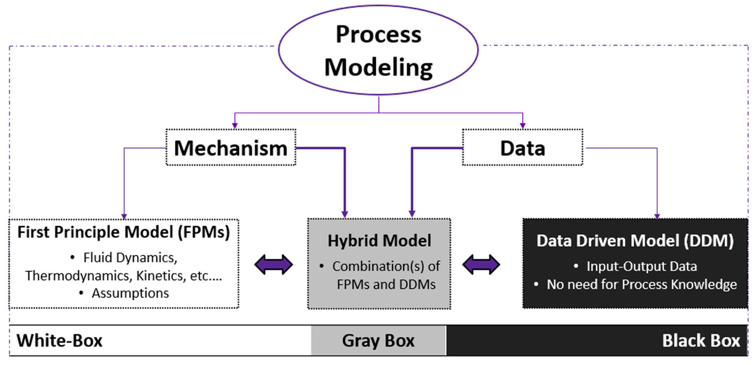Likewise, the study of optimization and control techniques used to enhance the operation of FCC units [3], coupled with accelerated computational development, has promoted the development of diverse data driven models (DDMs) and hybrid models (HMs) for the FCC process [5]. As shown in Figure 2, HMs, also known as “gray” box models, are a combination of FPMs—models that strongly rely on rigorously phenomenologically based fluid dynamics, thermal and kinetic mechanisms (knowledge) and DDMs—models that strongly depend on the process data [19]. Thus, HMs seek to compensate for the shortcomings of both FPMs and DDMs modeling approaches, using physicochemical constraints based on chemical process knowledge and data availability [20].

HMs for FCC units have primarily been developed using machine learning (ML) algorithms, combined with FPMs, to create simpler, more flexible, accurate, and interpretable models for industrial-scale units [20,21,22]. Some of the common applications of these ML algorithms reported in the technical literature are related to prediction, monitoring, control, and process optimization of FCC units [5]. One should note, however, that while there are several algorithms reported, it is difficult for one to decide which is most appropriate for a particular FCC unit or operating condition, considering the diversity of feedstocks, catalysts, and catalyst/oil ratio employed.

Furthermore, given the recent advances in numerical algorithms and the rapid increase in computational power [23], CFD methods for FCC applications are attracting great attention. This is the case, given the capacity of CFD to provide detailed gas-solid hydrodynamic information on fluidized beds much more quickly and economically than traditional experimental approaches [24]. Nevertheless, in the case of multiphase flows such as the ones present in FCC risers, it is well known that conventional CFD methods, which are based on a Eulerian-Eulerian framework, have limitations for modeling industrial-scale units. In view of this, the Eulerian-Lagrangian multiphase flow model developed by [25], designated as computational particle-fluid dynamics (CPFD), was used. This method has rapidly gained significant attention in recent years. This is the case, considering its capabilities for modeling scaled-up units as well as its ability to assist in the optimization of multiphase gas-solid catalytic reactors [26].

In view of the above, the purpose of this work is to develop and implement hybrid AI models for FCC. Thus, for this study, the following objectives were considered:

• The development and implementation of a reliable CPFD model to simulate an industrial-scale FCC riser reactor unit, including trustable kinetics determined in a CREC riser simulator.
• The establishment of AI-based models for the prediction of FCC riser reactor unit performance under a wide range of typical FCC riser operating conditions.
• It is our understanding that there is no study in the open literature addressing such a significant topic.

2. Methodology

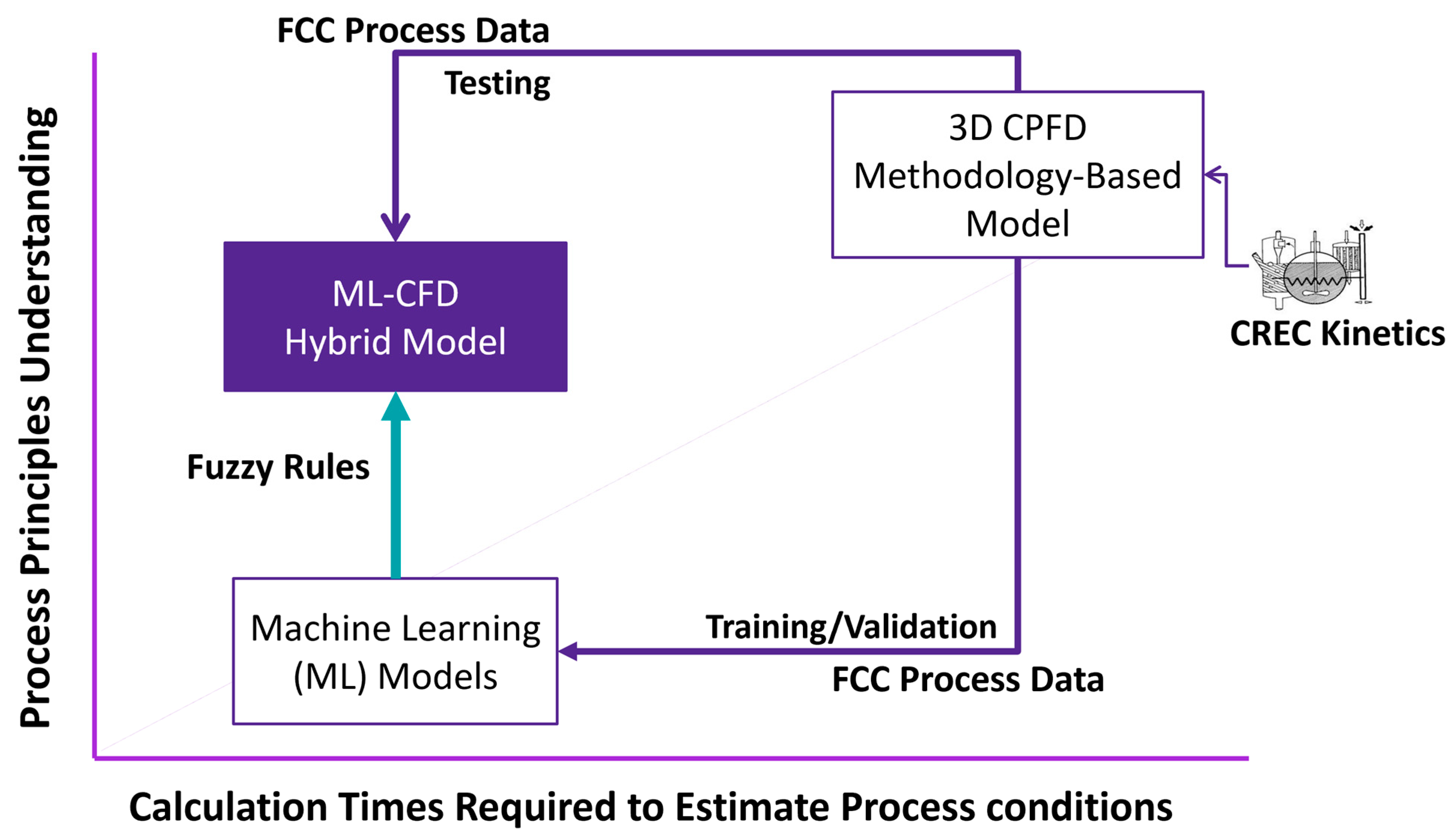
This paper introduces a hybrid model framework aimed at predicting six critical variables of FCC riser reactor unit processes at the industrial scale: (a) vacuum gas oil (VGO) conversion, (b) outlet riser temperature, (c) light cycle oil (LCO), (d) gasoline, (e) light gases, and (f) coke yields. This approach integrates a CPFD methodology with ML algorithms in order to establish correlations between the start-up conditions of the riser reactor and the resulting exit conditions of the catalytic process. This integration, as presented in Figure 3, allows the prediction of various possible operational scenarios with significantly shorter computational times than those required for CPFD computations, several minutes instead of several hours.

As described in Figure 3, when using 3D CPFD computations to simulate a commercial riser unit, a large database can be established. These 3D CPFD computations include VGO cracking kinetics derived from experiments in a minifluidized CREC riser simulator [27]. On the other hand, the ML model includes relevant fuzzy rules based on prior knowledge in order to define low, medium, and high fuzzy values for some of the variables considered in the proposed AI hybrid model.

On this basis, an AI hybrid model can be developed and implemented, as in this study, by using 90% of the available data for model training and 10% of the remaining data for AI hybrid model testing. Furthermore, for every AI model alternatively evaluated, a coefficient of determination ($R^2$) can be calculated in order to establish model reliability.

2.1. Computational Particle-Fluid Dynamics (CPFD)

The CPFD methodology involves a Lagrangian-Eulerian model for the purpose of fluid-particle flow simulation. This method uses a 3D multiphase particle-in-cell (MP-PIC) approach to solve the fluid and particle-governing equations, in three dimensions (

Table 1. MP-PIC Governing Equations.

Fluid-Phase Equations
Continuity equation of fluid phase:
$\frac{\partial \left({\epsilon }_f{\rho }_f\right)}{\partial t}+\nabla ·\left({\epsilon }_f{\rho }_f{u}_f\right)=\mathsf{\delta }\dot{m_p}$		(1)
Momentum equation of fluid phase:
$\frac{\partial \left({\epsilon }_f{\rho }_f{u}_f\right)}{\partial t}+\nabla ·\left({\epsilon }_f{\rho }_f{u}_f{u}_f\right)=$	$\left\{\begin{array}{c}Model A\\ -\nabla p_f+F+{\epsilon }_f{\rho }_{f}g+\nabla ·\left({\epsilon }_f{\tau }_f\right)\\ \\ Model B\\ -{\epsilon }_f\nabla p_f+F+{\epsilon }_f{\rho }_{f}g+\nabla ·\left({\epsilon }_f{\tau }_f\right)\end{array}\right.$	(2)
Enthalpy:
$\frac{\partial \left({\epsilon }_f{\rho }_f{h}_f\right)}{\partial t}+\nabla ·\left({\epsilon }_f{\rho }_f{h}_f{u}_f\right)={\epsilon }_f\left(\frac{\partial p}{\partial t}+u_f·\nabla p_f\right)+\varphi -\nabla ·\left({\epsilon }_{f}q\right)+\dot{Q}+S_h+\dot{q_D}$		(3)
Species transport:
$\frac{\partial \left({\epsilon }_f{\rho }_f{Y}_{f, i }\right)}{\partial t}+\nabla ·\left({\epsilon }_f{\rho }_f{Y}_{f, i }{u}_f\right)=\nabla ·\left({\rho }_{f}D{\epsilon }_f{\nabla Y}_{f, i }\right)+\mathsf{\delta }{\dot{m}}_{i, chem}$		(4)
Solid-Phase Equations
Liouville equation for finding the particle distribution function $f$, at each time:
$\frac{\partial f}{\partial t}+\nabla ·\left(f u_p\right)+{\nabla }_{u_p}·\left(f {\dot{u}}_p\right)=0$		(5)
Particle acceleration:
${\dot{u}}_p=\frac{{du}_p}{dt}=D_s\left(u_f-u_p\right)-\frac{1}{{\rho }_p}\nabla p_f+g-\frac{1}{{\epsilon }_p{\rho }_p}\nabla {\tau }_p+\frac{{\overline{u}}_p-u_p}{2{\tau }_D}$		(6)
Particle mass:
$\mathsf{\delta }\dot{m_p}=-\iiint f\frac{d{m}_p}{dt}{dm}_p{du}_p{dT}_p$		(7)
Particle volume fraction:
${\epsilon }_p=\iiint f\frac{m_p}{{\rho }_p}{dm}_p{du}_p{dT}_p$		(8)
Particle energy:
$C_V\frac{{dT}_p}{dt}=\frac{1}{m_p}\frac{{\lambda }_f N{u}_{f, p}}{2r_p}{A}_p\left(T_f-T_p\right)$		(9)
Fluid-Solid Interphase Equations
Momentum transfer between phases:
$F=\iiint f\left\{m_p\left[D_p\left(u_f-u_p\right)-\frac{1}{{\rho }_p}\nabla p\right]+u_p\frac{d{m}_p}{dt}\right\}{dm}_p{du}_p{dT}_p$		(10)
Particle-Particle Interaction Equation
Particle collision normal stress model:
${\tau }_p=\frac{P_p {\epsilon }_p^{\beta }}{\max \left[\left({{\epsilon }_{cp}-\epsilon }_p\right), \alpha (1-{\epsilon }_p)\right]}$		(11)

). This is performed to describe particle-fluid dynamics by using the averaged Navier–Stokes equations while involving a strong coupling with the particle phase [25,28]. When utilizing this approach, the solid phase transport equation is modeled by using a particle distribution function $f$, which is related to the product of the local particle density number, and the solid spatiotemporal properties, which include $x_p$ location, $u_p$ velocity, $m_p$ mass and $t$ time [24,29]: $f\left(x, u_p, m_p, t\right)$.

Thus, the CPFD methodology involves a discrete particle method, where the fluid phase is treated as a continuum and the catalyst particles (solids) are modeled using Lagrangian computational groups of particles, also called “clouds” or “computational parcels” [26]. These computational parcels are used to represent a certain number of actual catalyst particles that share the same properties, including uniform size, velocity, density, and temperature. This approach reduces computational effort while still accounting for catalyst-particle interactions. Moreover, since the CPFD method can work when using coarse meshes without loss of accuracy, long-time simulations are computationally affordable and relatively large time-steps can be adopted, which is not the case with conventional CFD methods [30].

In the present study, the CPFD methodology was developed and implemented using the Barracuda Virtual Reactor 22.0^® software, while accounting for:

• Fluid and catalyst particle properties,
• Fluid momentum balances using averaged Navier–Stokes equations coupled with the particle phase,
• Particle-fluid interactions using an energy minimization multiscale (EMMS) drag model,
• Particle interactions via a particle stress function ${\tau }_p$,
• Enthalpy balances, including gas and particles contributions,
• FCC catalyst particle size distribution,
• Suitable FCC VGO cracking reaction kinetics.

2.1.1. FCC Riser Unit

The primary objective of the FCC riser flow simulation was to calculate the concentrations of the principal oil species of interest and to evaluate the riser reactor performance. The FCC riser performance evaluation was based on (a) the converted VGO and (b) the various hydrocarbon product yields, the chemical species produced from either the primary VGO cracking or secondary cracking reactions of gasoline and cycle oil species. Considering that the extent of the cracking of hydrocarbon species mainly depends on the gas-solid residence time, the amount of available catalyst surface, the partial pressures of various hydrocarbon species, and the heat transfer from the catalyst [31], one must therefore account for the kinetics, the thermodynamics, and the fluid dynamics of VGO catalytic cracking in order to adequately represent the operating conditions in the FCC riser unit. This is required to accurately calculate the flow properties, including the gaseous species and the catalyst particle concentrations. In this regard, the CPFD simulations were developed for an industrial-scale FCC riser reactor unit, characterized by dimensions of 0.96–1.25 m in diameter with a height of 43 m. These specific unit measurements were taken from the FCC unit of the Petronor S.A. refinery, situated in Bilbao, Spain, as reported by [32].

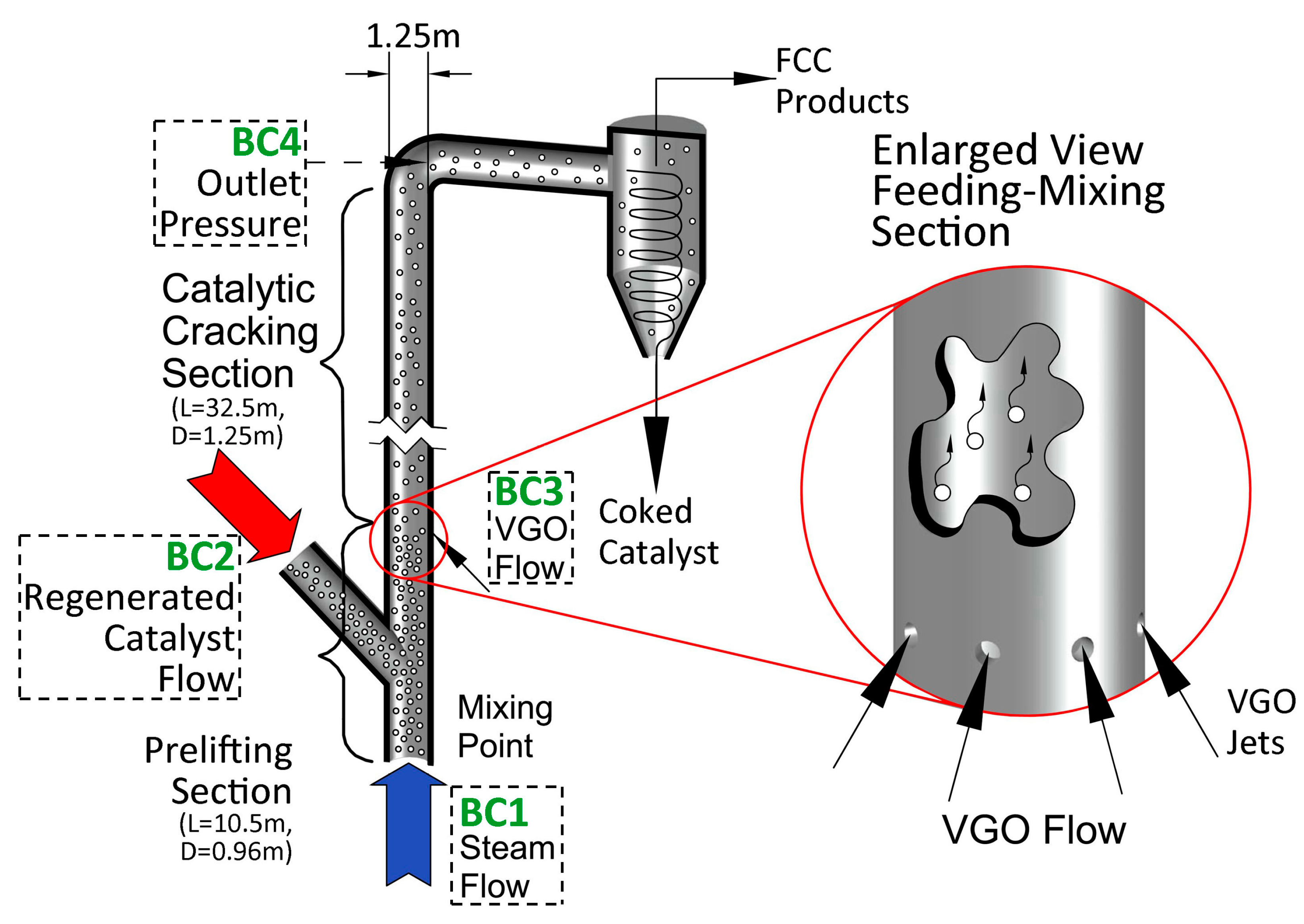
The 3D computational representation of the FCC riser’s geometry was discretized using a uniform grid size in every direction, amounting to ~300,000 computational cells. This large-scale FCC riser was comprised of a catalyst prelifting zone, followed by a gas oil feed injection zone housing 12 nozzles, and a main-riser zone encompassing a reactive length of 32.5 m. The processes selected for the CPFD simulation include the mixing of gas and solid phases and the cracking reactions involving both. Additional details of the simulated riser industrial scale unit are provided in the upcoming Figure 4.

2.1.2. Operating Conditions

The Barracuda Virtual Reactor 22.0^® software was employed to generate a bank of valuable FCC industrial-scale simulated data based on MP-PIC equations. This was achieved by evaluating a wide range of operating conditions, including critical variables affecting the performance of the FCC riser reactor unit such as catalyst-to-oil ratio (C/O), temperatures, and mass flows. In this regard, a total of 216 different inlet process condition combinations were considered in order to generate relevant and rigorously obtained process data suitable for AI-based models’ implementation. The variables and representative conditions used for all the simulations are reported in

Table 2. Factorial Simulation Design Table.

No.	Variables	Unit	Condition
			−1	0	1
1	Catalyst Mass Flow	kg/s	133.80	147.20	160.60
2	Catalyst Temperature	°C	-	650	700
3	VGO Mass Flow	kg/s	19.50	21.45	23.50
4	VGO Temperature	°C	210	230	250
5	Bottom Steam Mass Flow	kg/s	-	0.120	0.132
6	Bottom Steam Temperature	°C	-	250	300

.

For the described setup of all CPFD simulations, it was assumed that the riser reactor was initially filled with nitrogen and that the mass flow of VGO was zero. Thus, during the first seconds of the CPFD simulations, only nitrogen exits the riser reactor unit, while steam and catalysts move upward along the prelifting zone. Then, the steam-catalyst flow meets the feedstock that is injected via atomizing VGO droplets through the set of 12 feed oil injection nozzles. The VGO feed was set to increase gradually, starting at 6 s and reaching its final value at 13 s. For simplicity, it was assumed that the VGO entered the riser as a vapor. Likewise, an initial value of coke on the catalyst of 0.01 wt% was considered, and this for all the operating conditions simulated. In this respect, calculations were considered as simulating the start-up of the riser reactor until reaching 80 s of time-on-stream operation.

Figure 4 provides an overview of the boundary conditions (BCs) required for the CPFD simulations. These BCs were established at the entry and exit of the FCC riser unit as follows: (a) BC 1: set values for the steam pressure, the temperature, and the entry mass flow, (b) BC 2: set values for the catalyst pressure, temperature, and entry mass flow, (c) BC 3: set values for the VGO pressure, temperature, and entry mass flow, and (d) BC 4: set values for the outlet pressure of the gas-solid flow.

2.1.3. Catalytic Cracking Kinetics

In the FCC riser reactor, the catalytic cracking reactions produce a large number of molecules with a C₁–C₂₀ carbon number from a gas oil feedstock with a carbon number in the C₂₁–C₄₀ range. These changes in hydrocarbon molecular weight led to changes in the number of evolving moles of products, resulting in a significant change in volumetric flow along the height of the riser unit [33]. Therefore, the inclusion of adequate cracking kinetics to model not only the chemistry but also the hydrodynamics along the riser is of high importance.

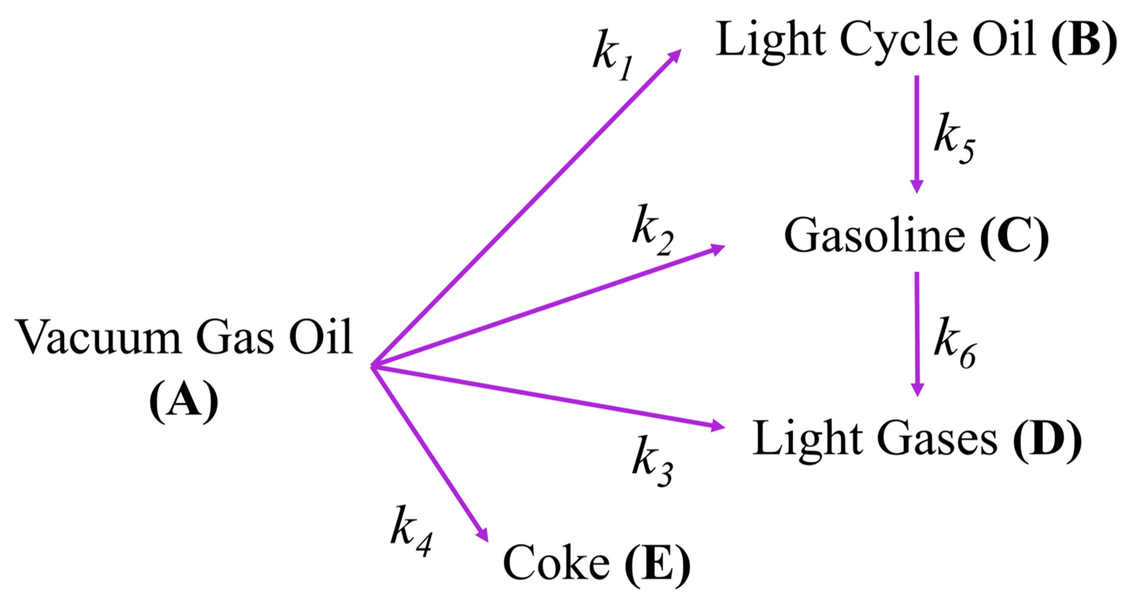
For the catalytic cracking, 5-lump kinetics for VGO catalytic cracking, including catalyst deactivation, are implemented. The lumped kinetic model considers the presence of five pseudo-hydrocarbon components in the multiregime riser reactor, which are A: VGO (C₂₆–C₄₀), B: LCO (C₁₂–C₁₆), C: gasoline (C₅⁺–C₁₂), D: light gases (C₁–C₄), and E: coke (Figure 5).

Thus, the VGO cracking kinetics are incorporated into the CPFD methodology based on an average cell size calculation. This means that average properties for both the fluid and the particle phase involved in the chemical rate equations are calculated by interpolating the discrete computational particle properties to the cell in the grid. In view of this, reaction rates are established in each cell by solving a set of ordinary differential equations [28]. Based on this, the source/sink term of the reaction rate, for each lump $i$ ($\mathsf{\delta }{\dot{m}}_{i, chem}$) in Equation (4), is calculated by [34]:

$$\mathsf{\delta }{\dot{m}}_{i,chem}=\sum {\mathsf{\delta }}_j{r}_j=\sum {-\mathsf{\delta }}_j{k}_{0j}\exp \left(\frac{-E{a}_j}{R_{g}T}\right)\frac{{\rho }_f}{{\epsilon }_f}{m}_p{Y}_{f,i}^n\phi$$

(12)

where ${\mathsf{\delta }}_j$ is the stoichiometric coefficient of the lump $i$ in the reaction path $j$; $r_j$ is the apparent rate of the $j$ reaction path; $Y_{f,i}$ and $m_p$ are the mass fraction of lump $i$ and the catalyst mass per unit cell, respectively; $R_g$ is the universal gas constant (8.314 J∙mol/K); $T$ is the mean temperature of the fluid and solid phases; $n$ is the reaction order; and where $k_0$ and $Ea$ are the pre-exponential factor and activation energy, respectively, for each reaction path $j$.

In this study, the kinetic parameter values involved in the cell size calculations, were taken from the ones reported by [27], obtained from experimental cracking runs developed with a VGO feedstock, in a CREC riser simulator. The main properties of the proposed lumps and the kinetic parameters values considered for this study are available in Appendix A, in

Table A1. Properties of Proposed Lumps.

Lump	Range of Hydrocarbons	Boiling Point Range (°C) at 1 atm	Molecular Weight (g/mol)
Gas Oil	>C20	>342.7	397
Light cycle Oil	C12–C20	216.3–342.7	226
Gasoline	C5–C12	36.1–216.3	114
Light gases	C1–C4	<36.1	46
Coke			800

and

Table A2. Kinetic Parameters for Gas Oil Catalytic Conversion [27].

	Value	95% CFL	Units
k1	1.16 × 10−2	±2.1%	m6/(kgCrystallite molGasOil s)
E1	97.01	±11.9%	kJ/molGasOil
k2	5.04 × 10−3	±2.4%	m6/(kgCrystallite molGasOil s)
E2	120.61	±4.1%	kJ/molGasOil
k3	4.06 × 10−3	±3.1%	m6/(kgCrystallite molGasOil s)
E3	136.17	±4.8%	kJ/molGasOil
k4	1.49 × 10−3	±4.0%	m6/(kgCrystallite molGasOil s)
E4	139.65	±5.1%	kJ/molGasOil
k5	7.60 × 10−2	±6.4%	m3/(kgCrystallite s)
E5	90.43	±15.4%	kJ/molLCO
k5	4.70 × 10−2	±8.3%	m3/(kgCrystallite s)
E6	82.86	±21.6%	kJ/molGasoline
$\mathsf{\lambda }$	26.1	±4.5%	-

, respectively.

2.2. AI-Based Model

The implementation of AI-based models as chemical process performance evaluators is receiving increasing attention due to their robustness, simple formulation, ease of design, and flexibility [20]. As previously mentioned, AI techniques can overcome the drawbacks of FPMs when dealing with complex and nonlinear systems. Consequently, the application of AI in modeling, optimization, process control, detection, and diagnosis of failures has increased dramatically in recent years [35]. Furthermore, one of the branches of AI that is most directly and immediately applicable to chemical process systems is ML algorithms. These have been investigated for more than 30 years by AI researchers in chemical engineering. Remarkable results have been obtained despite the remaining phenomenological knowledge gaps with these algorithms [19,36].

In general, the tasks of AI-based models developed with ML algorithms share certain common characteristics. They all involve pattern recognition, reasoning, and decision-making. In the case of chemical process systems, ML algorithms often face ill-defined problems, noisy data, model uncertainties, nonlinearities, and the need for quick solutions to complex conditions [36]. In this regard, one of the most important steps in developing an efficient AI-based model is to define the appropriate input/output variables of the system to be modeled [35]. Based on this, AI-based models can be used to analyze chemical process behaviors by mapping the process inputs-outputs [19].

In this study, a set of input features consisting of six independent process inlet conditions and two dependent operating conditions is proposed as the basis for the AI-based model predictions, as summarized in

Table 3. Proposed Predictors for AI-Based Model.

No.	Condition	Units	Type
1	Catalyst Mass Flow	kg/s	Independent
2	Catalyst Temperature	K
3	VGO Mass Flow	kg/s
4	VGO Temperature	K
5	Bottom Steam Mass Flow	kg/s
6	Bottom Steam Temperature	K
7	C/O Ratio	kg Catalyst/kg VGO	Dependent
8	Mixing Point Temperature	K

. These eight predictors are chosen to be used for the estimation of six conditions of interest in the operation of the industrial-scale FCC riser reactor units. These conditions are: (a) the VGO conversion, (b) the LCO selectivity, (c) the gasoline selectivity, (d) the light gases selectivity, (e) the coke, and (f) the fluid outlet temperature.

For the development of the AI-based model, a dataset generated for the FCC riser reactor operation through CPFD simulations is imported into the MATLAB environment, where the data is processed as follows:

• First, the sets of operating conditions leading to temperatures at the mixing bottom section higher than 570 °C or lower than 510 °C are discarded from the original dataset. This was performed by considering the limits of the temperature range used for the VGO cracking kinetics as reported by [27].
• Then, a “hold-out” method considered 90% of all the data randomly selected for AI training. The remaining 10% of data is kept aside to be used for the final testing of the AI model.
• In addition, the entire training data is split into 10 different subsets, or folds. This is performed for the K-fold cross-validation implementation and based on the reduced number of data points available, as recommended by [37]. Regarding the selected 10-folds, 90% of the data are considered for AI training and 10% for validation.
• Following this, the AI model is developed and validated for each one of the selected K-folds.
• Once this step is completed, the various AI model parameters established for each one of the K-folds are averaged with the selection of the best fitting parameters, providing a designated “ensemble” model with the corresponding statistical indicators.
• Finally, the developed “ensemble” model was evaluated by comparing it with 10% of the original data randomly chosen, as described in step 2.

2.2.1. Artificial Neural Network (ANN)

Since the development of the backpropagation algorithm to train feedforward neural networks (FNNs) in 1986 and the research followed up into neural networks in the early 1990s [36], ANN has been among the ML algorithms most widely used in various industrial processes. This is given their great ability to “learn” hidden patterns in input and output process data [5]. Furthermore, due to their high potential to handle nonlinear relationships through different activation functions, there has been considerable interest in the use of neural networks in the different fields of chemical processes [35]. Likewise, within technical literature, FNN has been one of the most successfully implemented topologies and currently continues to be one of the most favorable approaches for modeling tasks [21].

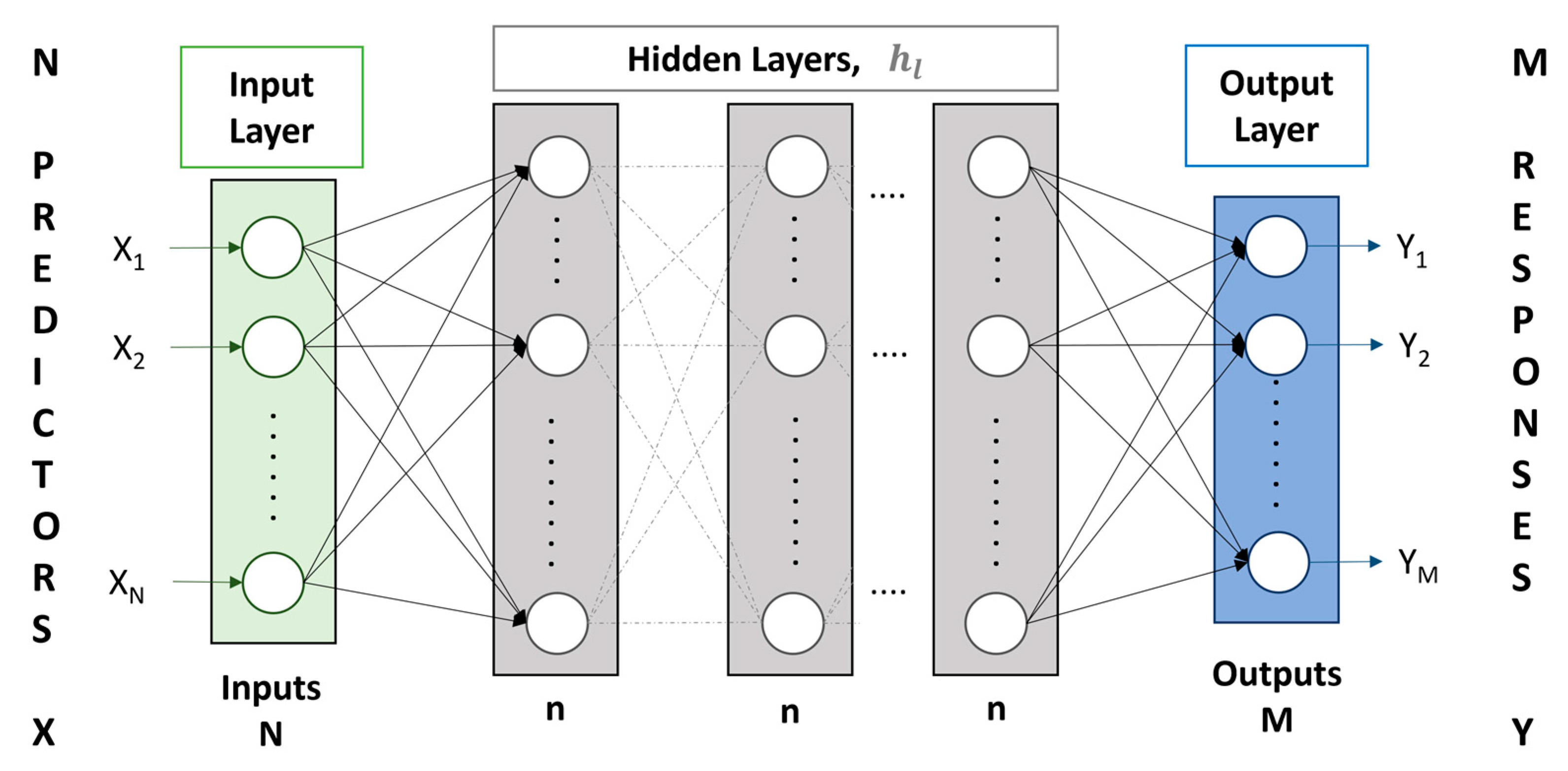
In general, ANNs are inspired by the structure and function of the human brain. In ANNs, simple interconnected neurons or nodes, functioning as processors, are organized into three types of layers: the input layer, the output layer, and the hidden layer [20,38], as illustrated in Figure 6. These connections between nodes are quantified by weights, which determine the strength of each connection. Moreover, each neuron or node in the network is equipped with a bias term that plays a role in shaping the behavior of the individual neurons and contributes to the overall network performance.

As described by [39], the weights and biases of a FNN are adjusted via forward and backward calculations during the training phase of the ANN. This can be performed iteratively until a predefined loss function is minimized [37]. Therefore, the selection of the proper hyperparameters plays a role of great importance in effectively guiding this iterative training process. Taking this into consideration, the performance of different FNN configurations was evaluated using an averaged coefficient of determination ($R^2$), as an evaluation reference:

$$R^2\left(y,\widehat{y}\right)=1-\sum _{i=1}^n\frac{{\left(y_i-{\widehat{y}}_i\right)}^2}{{\left(y_i-\overline{y}\right)}^2}$$

(13)

where $y_i$ is the output variable from the CPFD data, ${\widehat{y}}_i$ is the output variable of the predicted data, and $\overline{y}$ is the average of $y_i$. The various ANN hyperparameters adopted in the present study, to develop a multiple output FNN, are reported in

Table 4. Hyperparameters used to Develop FNNC. Notes: Selected Hyperparameter Names as Designated in the MATLAB Environment.

Type	Hyperparameter	Value	Description
Performance	performFcn	RMSE	This provides the root mean square error (RMSE) as performance function.
	performParam.regularization	0.15	This considers a performance ratio for regularization.
	performParam.normalization	‘standard’	This provides a standard normalization of the target variables values.
Training	trainParam.goal	0.01	This considers a RMSE desired value as the goal for the training.
	trainFcn	traingdx	This provides training by using gradient descent with momentum and adaptive learning rate backpropagation
	trainParam.lr	0.01	This considers an initial learning rate for the training.
	trainParam.lr_inc	1.005	This enhances training by employing an increase ratio in the learning rate.
	trainParam.lr_dec	0.05	This enhances training by employing a decrease ratio in the learning rate.
	trainParam.mc	0.75	This incorporates a momentum value for updating weights during training.
	divideFcn	‘dividerand’	This involves training with a data division function for training and validation.
	divideParam.trainRatio	0.9	This considers a data split ratio for training.
	divideParam.valRatio	0.1	This considers a data split ratio for validation.
	trainParam.max_fail	20	This considers a maximum validation cap for failures.
Architecture	transferFcn	‘tansig’	This involves a hyperbolic tangent sigmoid activation function for nodes connections.
	Hidden Layers	1, 2, 3	Up to a maximum of three hidden layers are considered.
	Hidden Layers Nodes	1–12	Up to a maximum of 12 nodes for each hidden layer are considered.
	Parameters	<200	Up to a maximum of 200 parameters are selected to prevent overparameterization.

. These hyperparameters, including learning rates and activation functions, were systematically tuned for optimal performance in minimizing the specified loss function during training. One should note that a deliberate choice was made to limit the number of parameters in the FNN models, to a maximum of 200. This parameter capping considers the dataset available: 216 operating conditions and 6 output variables. Therefore, this parameter capping served the dual purpose of constraining model complexity and avoiding parameter overfitting.

2.2.2. Fuzzy Rules

In general, a chemical process can be rigorously represented in different ways. Thus, it is important to distinguish between mechanistic descriptions, heuristic descriptions, and pure process data correlations [40]. Mechanistic descriptions rely on rigorous mathematical equations grounded in physical principles. Heuristic descriptions often employ empirical rules based on prior knowledge. Pure process data correlations utilize observed data. These different approaches offer flexibility and applicability, in various scenarios, depending on the level of understanding and the availability of data.

When considering the implementation of heuristic descriptions, fuzzy rule-based systems have been proved to be powerful tools to describe the dynamic behavior of processes [40]. Fuzzy logic, which is a multivalued logic system, is particularly well-suited to handle heuristically defined rules and knowledge [41]. Defined fuzzy sets normally allow variables to take on values within defined ranges, such as low, medium, and high. The advantages of using such descriptions include the ability to capture and bound process topology, representing cause-effect relationships between variables, while avoiding the issues that arise when numerically solving complex mathematical models, through numerical simulation [16]. Furthermore, defined fuzzy sets are particularly useful for systems with rapidly changing process variables, allowing monitoring and bounding variables with high and low values to prevent miscalculation issues.

In this context, the following fuzzy sets were defined in the present study, to categorize the mixing temperature ($T_{mix}$) and C/O ratio:

Temperature:	$T_{mix}<530$	Low Temperature Regime (LTR)
	$530<T_{mix}<550$	Medium Temperature Regime (MTR)
	$T_{mix}>550$	High Temperature Regime (HTR)
C/O Ratio:	$C/O<6$	Low CO Ratio
	$6<C/O<7.5$	Medium CO Ratio
	$7.5>C/O$	High CO Ratio

These fuzzy rules are selected to classify the mixing temperature and C/O ratio values into distinct operating regimes. Subsequently, these fuzzy sets are applied to enhance the predictive performance of the FNN models, which were originally trained using direct $T_{mix}$ and C/O ratio values. The results obtained are discussed below.

3. Results and Discussion

3.1. CPFD Simulation Results

The CPFD simulations developed in the Barracuda Virtual Reactor 22.0^® software were used to investigate the gas-solid flow behavior, as well as the temperature distribution, inside the industrial-scale FCC riser reactor unit. These simulations were run using parallel computing and GPU acceleration via a Graham Cluster, which is one of the general-purpose clusters of the Digital Research Alliance of Canada (the Alliance). The contours generated from the results obtained when evaluating the first set of proposed inlet conditions (

Table 5. First Set of Inlet Conditions (Simulation ID: 1).

Condition	Value	Units
Catalyst mass flow	133.80	kg/s
Catalyst temperature	923	K
VGO mass flow	19.50	kg/s
VGO temperature	483	K
Bottom steam mass flow	0.120	kg/s
Bottom steam temperature	523	K

) are presented below in Figure 7, Figure 8, Figure 9 and Figure 10.

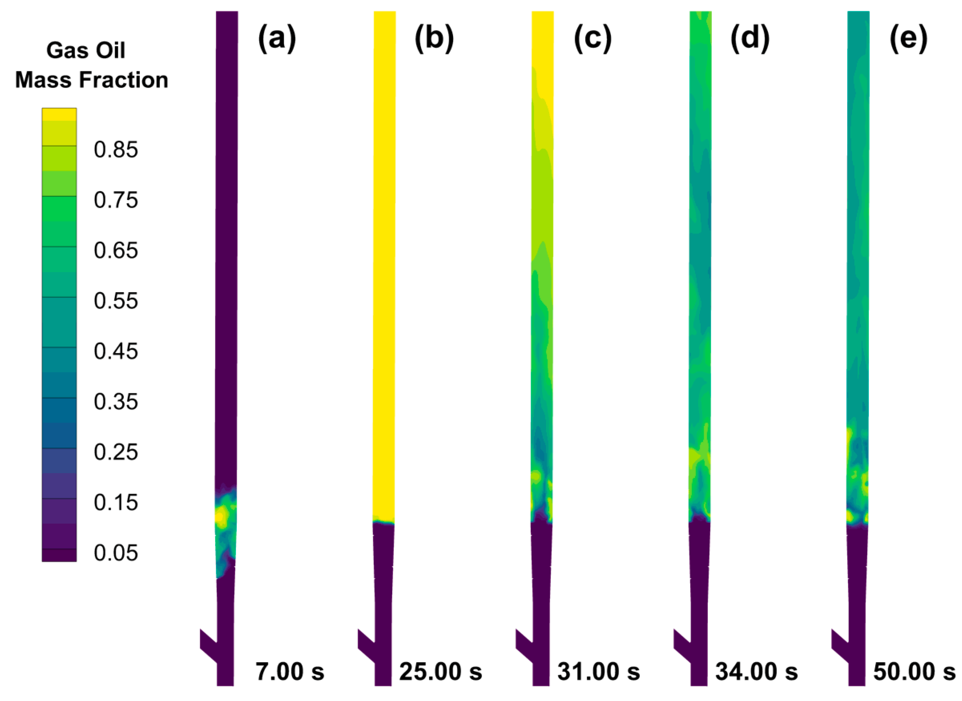
As illustrated in Figure 7, the mass fraction of VGO initially remains at a value of zero, while exhibiting a notable increase at 7 s into the simulation. This rise in the VGO mass fraction at the mixing level locations corresponds to the initiation of the feeding of VGO to the FCC unit. By 25 s of reaction time in the simulations, the length of the reactor (reaction section) is entirely filled with VGO. However, at approximately 30 s, the mass fraction of VGO begins to decrease. This decrease coincides with the contact between the catalyst particles and the VGO injected, leading to catalytic cracking reactions as a result of lower VGO fractions along the riser unit. Finally, by 50 s, the VGO distribution stabilizes along the riser reactor’s outlet, showing the establishment of a quasi-steady state operation.

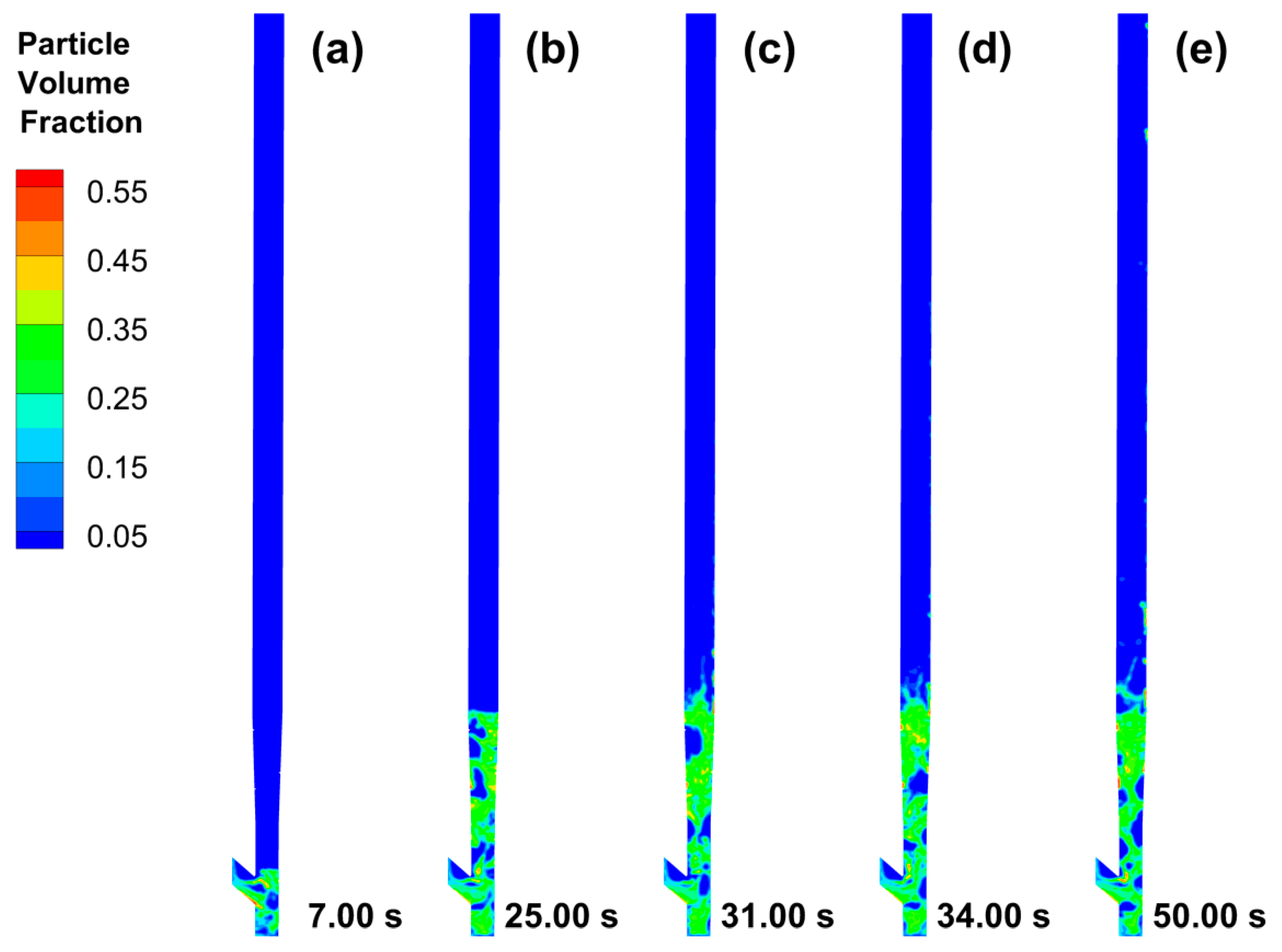
At the beginning of the simulations, catalyst particles are continuously fed into the riser reactor. Then, as shown in Figure 8, 7 s of simulation, the catalyst particles occupy only a small section of the prelifting zone, with very low solid fraction levels, in the riser. At 25 s, however, the catalyst particles can be seen to be well distributed in a densified phase section throughout most of the prelifting zone. After 30 s, catalyst particles reach the mixing point and start interacting with the VGO, causing particles to be lifted by the VGO injections. As a result, and following the 30 s simulation time, two distinct regions are consistently observed: a dense phase with a high catalyst particle volume fraction (lower riser section), and a diluted phase with a very low catalyst particle volume fraction (higher riser section), as expected, in this type of FCC riser reactor units.

Figure 9 and Figure 10 report the temperature dynamics, within the riser reactor unit, during a CPFD-Barracuda simulations. This analysis sheds light on the intricate interplay between temperature profiles, and their correlations with the VGO injected and the catalyst distribution, as well as the catalytic cracking kinetics. This provides valuable insights into the reactor’s behavior.

As shown in Figure 9, throughout the entire simulation period, the prelifting zone consistently maintains the highest thermal level, along the riser reactor. This higher temperature is attributed to the substantial contribution of heat from the regenerated catalyst particles (e.g., 923 K). As the simulation progresses, especially after the 30 s of simulation, a temperature decreasing gradient along the riser becomes apparent. Specifically, higher temperatures are observed around the mixing point at the bottom of the riser, while lower temperatures are observed towards the riser reactor outlet. This temperature reduction is primarily attributed to the endothermic nature of catalytic cracking reactions. These reactions consume thermal energy, resulting in a cooling effect along the reactor unit.

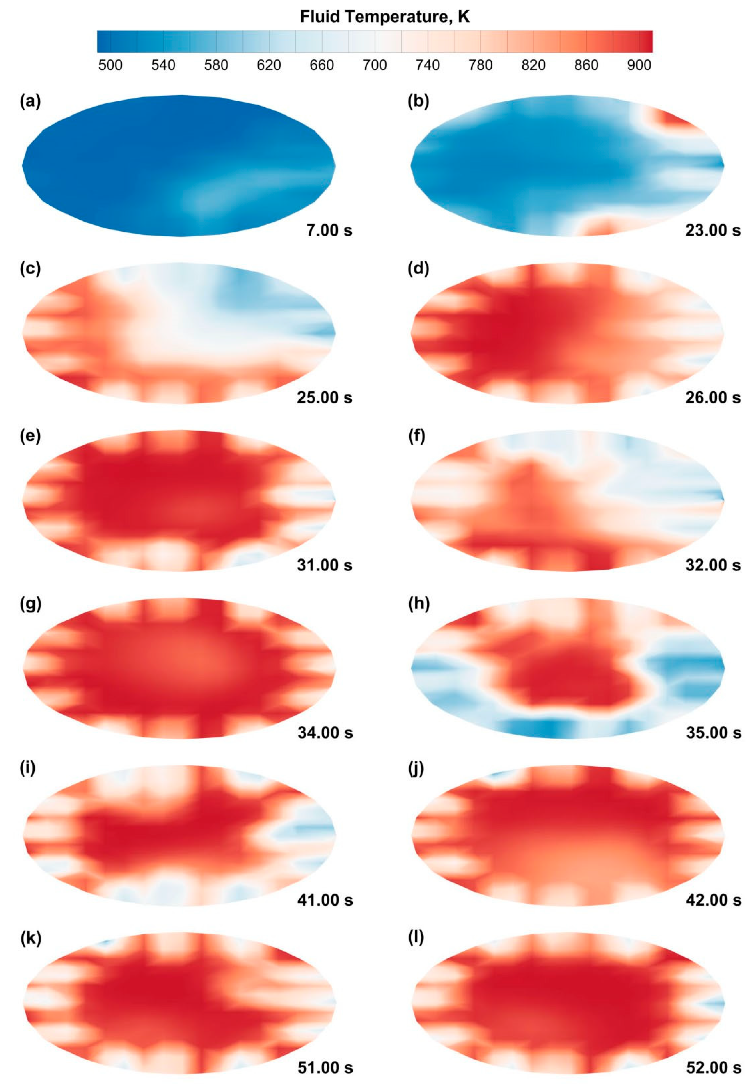
When analyzing the behavior of temperature at the mixing bottom section (Figure 10), some important observations emerge. First, during the initial seconds of the simulation, the mixing section temperature remains quite uniform. However, starting at approximately 7 s, temperature fluctuations become evident. This corresponds with the feeding of the VGO interacting with the catalyst-steam flow. At approximately 23 s of simulation time, the steam and hot regenerated catalyst particles reach the mixing section, moderating the endothermicity of the cracking reactions. Furthermore, by 25–26 s, catalyst particles completely fill the mixing plane, with a pronounced lower temperature being observed in proximity to the VGO injection nozzles. Beyond the 31 s, the presence of the hot catalyst continues to influence riser temperature dynamics, albeit with flow fluctuations with temporal variations, of the temperature distribution. Remarkably, in the latter stages of the simulation, a persistent temperature pattern emerges, suggesting the attainment of a dynamic equilibrium. These findings underscore the intricate interplay between catalyst dynamics and temperature, emphasizing the necessity for in-depth investigations into catalyst recirculation and catalyst/oil ratios and their consequences on reactor performance, and product quality, within FCC units.

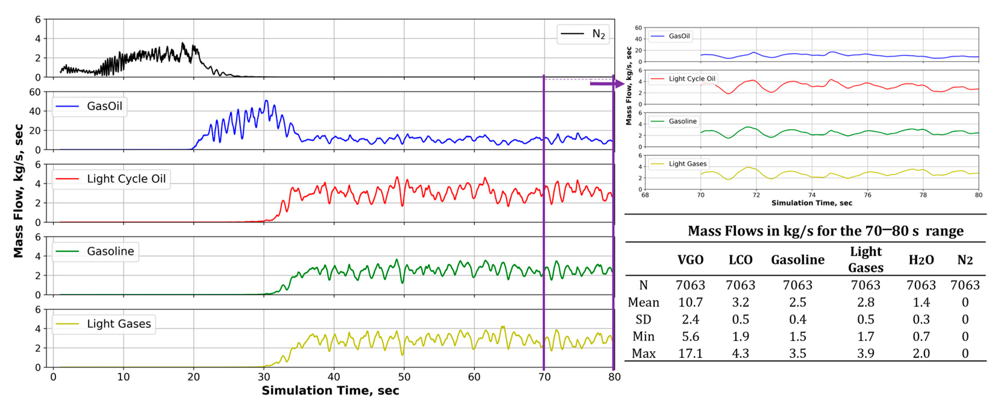
On the other hand, the data generated during the computational calculations were analyzed in detail, through individual data files analysis, for each simulation. This was carried out by using the Python language. With these data files, it was possible to calculate the variables of interest, at the riser reactor’s outlet, and at different simulation times. Consequently, given the fact that the mass fluxes of the various chemical species “stabilized” after 60 s of simulation, for most of the inlet conditions evaluated, the calculations of VGO conversion (Equation (14)), products selectivity (Equation (15)) and coke deposition (Equation (16)), were developed for the last 10-s of each simulation (70–80 s). The CPFD results obtained, and the calculated variables of interests acquired for the first set of proposed inlet conditions (Table 5), are presented in Figure 11 and in

Table 6. Estimated Values following CPFD Simulations.

Variable of Interest	Value	Units
VGO conversion	45.19	%
LCO selectivity	36.34	%
Gasoline selectivity	28.87	%
Light gases selectivity	31.60	%
Mixing temperature	785	K
Outlet temperature	757	K

, respectively.

$$X_{VGO}=\frac{F_{VG{O}_0}-F_{{\left.VGO\right|}_{70–80 \mathrm{s}} }}{F_{VG{O}_0}}$$

(14)

$$S_i=\frac{F_{{\left.i\right|}_{70–80 \mathrm{s}} }}{F_{VG{O}_0}-F_{{\left.VGO\right|}_{70–80 \mathrm{s}} }}$$

(15)

$$C_{Coke}=\frac{F_{{ \left.Coke\right|}_{70–80 \mathrm{s}} }}{{F }_{{\left.Solids\right|}_{70–80 \mathrm{s}}} }$$

(16)

where $F_{VG{O}_0}$ and $F_{VGO}$ are the VGO inlet and outlet mass flows, respectively, $F_i$ is the mass flow of each product $i$, and $F_{Solids}$ and $F_{Coke}$ are the total mass flows of solids and coke, respectively.

Data Quality Evaluation

The values obtained, based on the CPFD simulation results, were analyzed using MATLAB R2022b. As reported in

Table 7. Summary of Hydrocarbon Lump Results Obtained with the CPFD Simulation.

Variable of Interest	Raw Data from CPFD				Units
	Max	Min	Mean	SD
VGO conversion	61.82	36.57	47.84	4.86	%
LCO selectivity	42.17	19.36	31.15	4.01	%
Gasoline selectivity	32.69	21.50	27.54	1.80	%
Light gases selectivity	40.81	23.57	33.15	3.48	%
Mixing temperature	869	754	814	24	K
Outlet temperature	831	742	785	20	K
Coke on catalyst	0.66	0.5	0.58	0.05	%

, the CPFD predictions showed a moderate to high level of VGO conversion (36.57% to 61.82%). Likewise, outlet temperatures were shown to be in a moderate range (785–831K), suitable for adequate FCC riser reactor operation. In the case of selectivities, various product selectivities, as reported in Table 7, indicated good riser efficiency with different products of interest formed as desired. In addition, considering that the initial value of coke-on-catalyst in the CPFD simulations was 0.01%, one can conclude that the obtained coke-on-catalyst values (0.5 to 0.66%) reflected the expected low to moderate accumulation of coke on the catalyst surface as a result of the catalytic cracking process.

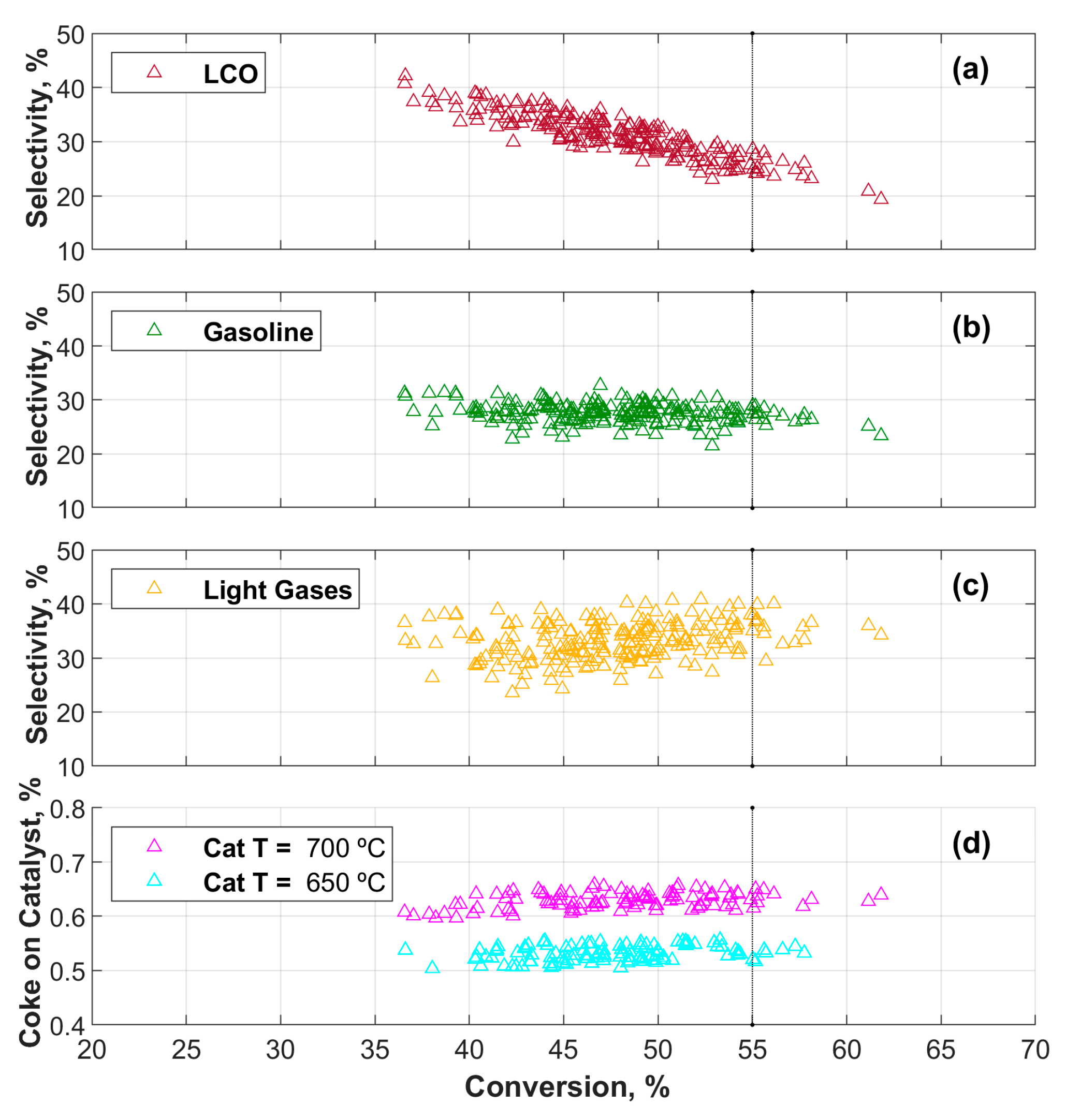
Figure 12 provides a comprehensive report of product selectivities and coke deposition in the FCC riser reactor unit, offering key insights into the interplay of these variables with VGO conversion. First, the LCO selectivity exhibits a clear trend, indicating that as VGO conversion rates rise, LCO selectivity values tend to decrease. Conversely, gasoline selectivity remains relatively stable along the conversion axis, with minor variations. Meanwhile, the selectivity towards light gases showcases an interesting trend consisting of increasing values at higher VGO conversions, albeit with a wider distribution. This behavior in the product selectivity indicates that there is a tendency to overcrack in the FCC riser reactor unit under the highest VGO conversion conditions. This leads to the production of a greater proportion of lighter hydrocarbon fractions. Moreover, the distribution of the coke-on-catalyst reveals a segregation pattern, with higher values being associated with elevated catalyst inlet temperatures. This segregation underscores the significance of catalyst temperature control in managing coke deposition efficiently and optimizing reactor performance.

3.2. Machine Learning (ML) Results

In this research, a rigorous approach employed to evaluate the performance of various FNN architectures was implemented using the dataset generated with the help of CPFD as the basis for model testing. This was accomplished by creating an averaged FNN ensemble based on the best parameters obtained during the training of the 10 k-folds, for each architecture. This evaluation method provided a robust understanding of the performance of the AI model, accounting for the variability introduced by different datasets. By assessing the model’s predictions across multiple folds, the risk of overfitting was mitigated, and led to a more accurate representation of its generalization capabilities.

One noteworthy outcome of this evaluation is the striking differences observed in the overall root mean square error (ORMSE) for each averaged FNN architecture. These differences in the ORMSE underscore the sensitivity of models to the underlying data distribution and the architecture of the neural networks. The variations in the ORMSE suggest that the choice of hidden layers and neuron numbers significantly impacts the model’s predictive accuracy. Variations were observed not only in the ORMSE values but also in the $R^2$, for each product yield prediction. The results obtained for the best five averaged FNN architectures are presented in

Table 8. Architecture and Performance Metrics of Top Five Averaged Neural Networks.

		FNN1	FNN2	FNN3	FNN4	FNN5
Architecture	Hidden Layers	1	2	2	3	3
	Nodes	[10]	[6, 9]	[10, 5]	[3, 10, 7]	[6, 10, 4]
	Parameters	156	177	181	192	198
$ORMSE$		2.38	2.00	1.98	2.37	2.24
$R^2$	VGO Conversion	0.86	0.86	0.85	0.80	0.85
	LCO selectivity	0.80	0.85	0.84	0.81	0.86
	Gasoline selectivity	0.09	0.15	0.17	0.23	0.29
	Light Gases selectivity	0.65	0.69	0.66	0.68	0.68
	Outlet Temperature	0.96	0.97	0.98	0.96	0.96
	Coke on Catalyst	0.96	0.99	0.99	0.99	0.99
Average $R^2$		0.721	0.752	0.749	0.745	0.772

.

On average, the models considered exhibit consistent performance across product yield predictions. Notably, these architectures vary in their numbers of hidden layers and neurons. Among them, the FNN3 and the FNN2 stand out, with the lowest ORMSE values of 1.98 and 2.00, respectively. This shows the superior predictive accuracy of the 2-hidden-layer FNN model. Remarkably, these FNNs maintain a relatively lean architecture in comparison to more complex FNN architectures, such as the FNN4 (192 parameters) and the FNN5 (198 parameters) models.

Moreover, when examining the $R^2$ values, it is apparent that each architecture exhibits differences, in its ability to fit the data. For instance, the 1-hidden-layer FNN1 excels in modeling the VGO conversion in the riser reactor unit, attaining an $R^2$ of 0.86, while it lags slightly in the gasoline selectivity prediction, with an $R^2$ of 0.09. In the case of the 2-hidden layers of the FNN2 and the FNN3, one can note that they perform similarly to the FNN1 in terms of VGO conversion, while showing improvements in gasoline selectivity predictions. Likewise, more complex models such as FNN4 and FNN5, also show enhancements in terms of the estimation of gasoline selectivity. However, these observed improvements, in the average $R^2$ are small when compared to the 2-hidden-layer FNNs. These results emphasize the sensitivity of FNN models to architecture choices and data distribution, underscoring the need for careful selection and optimization when applying neural networks in predictive modeling. In fact, differences in $R^2$ values provide valuable insights into how architectures perform with respect to specific target variables, making it clear that a one-size-fits-all approach may not be ideal for predictive tasks.

Fuzzy Rules Results

Table 9. Architecture and Performance Metrics of Averaged Neural Networks with Fuzzy Set Integration.

		FNN1	FNN2	FNN3	FNN4
Architecture	Hidden Layers	1	2	2	2
	Nodes	[10]	[5, 5]	[5, 8]	[8, 5]
	Parameters	196	131	167	185
$ORMSE$		1.78	1.93	2.02	1.93
$R^2$	VGO Conversion	0.84	0.85	0.85	0.89
	LCO selectivity	0.79	0.84	0.88	0.89
	Gasoline selectivity	0.37	0.14	0.68	0.49
	Light Gases selectivity	0.80	0.69	0.78	0.79
	Outlet Temperature	0.99	0.98	0.96	0.97
	Coke on Catalyst	0.99	0.99	0.99	0.99
Average $R^2$		0.796	0.749	0.859	0.836

reports the modeling results of four different FNN models, integrating fuzzy set conditions into the mixing temperature and the C/O ratio. The fuzzy sets were integrated into the FNN models as dummy variables, leading to the introduction of six new model variables in the input layer of the FNN architectures. These new variables replace the direct values of the $T_{mix}$ and the C/O ratio, resulting in an increased number of parameters due to the addition of new nodes and needed connections with other layers. In the case of FNN1, this change in the input layer led to an increase in the number of parameters from 156 in Table 8 to 196 in Table 9. Consequently, when this change was applied to the FNN2, FNN3, FNN4, and FNN5 models, these models exceeded their proposed targets of 200 parameters, as described in Section 2.2.1. Thus, as a result, 3-hidden-layer FNN architectures were no longer considered, and instead, three new 2-hidden-layer FNN architectures were used for further model discrimination analysis.

It is shown in Table 9 that the proposed AI architecture changes enhance the overall performance predictions. In fact, the ORMSE display values are in the 1.78–2.02 range, which is a narrower range than the 1.98–2.38, shown in Table 8. Likewise, the 0.859 and 0.836 $R^2$ for the new 2-hidden FNN3 and FNN4, respectively, show significant increases when compared to the 0.745 and 0.749 values in Table 8. One should note that these $R^2$ increases are mainly due to the improvement in the prediction of the distribution of gasoline and light gases selectivity values by the new FNN models. These prediction enhancements can also be appreciated when comparing light gases and gasoline lumps for the FNN1 model, as reported in Table 8 and Table 9. In these tables, one can see that the $R^2$ for gasoline selectivity and light gases selectivity increase from 0.09 and 0.65 to 0.37 and 0.80, respectively. Therefore, one can conclude that there is a positive impact for incorporating fuzzy rules and new model variables into the FNN, as part of the HM architecture proposed in this work.

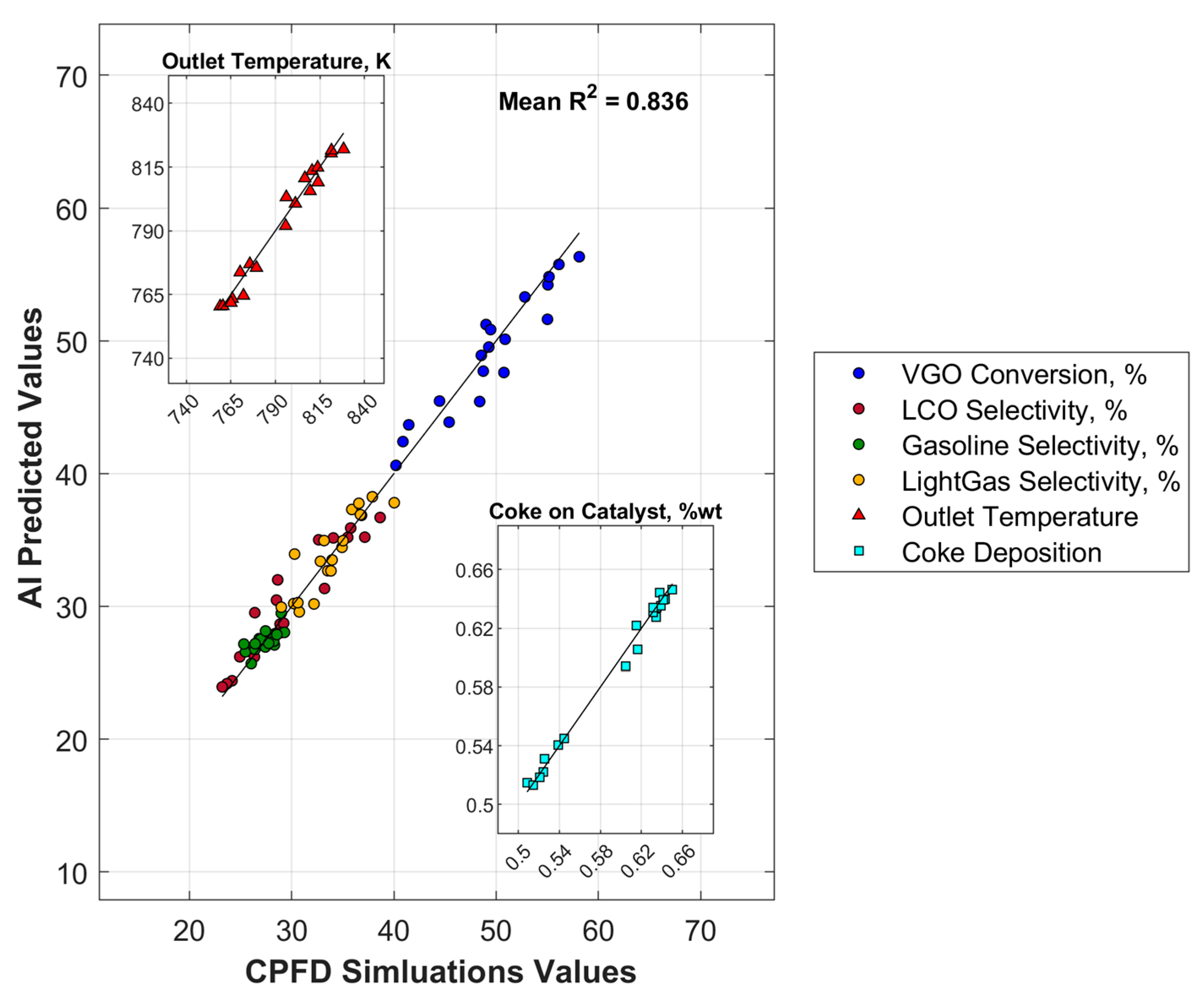
Finally, and on this basis, the most suitable FNN architecture was chosen based on the balance of AI model complexity and performance. This is the FNN4 model, which includes two hidden layers with eight and five neurons for each layer. Figure 13 reports the excellent predictions obtained for all the output variables considered here: (a) outlet riser temperature, (b) VGO conversion, (c) LCO selectivity, (d) gasoline selectivity, (e) light gases selectivity, and (f) coke-on-catalyst.

As depicted in Figure 13, the FNN hybrid model, including fuzzy constraints, aligns closely with the CPFD-Barracuda estimations. These small deviations are associated with the unavoidable sources of experimental and computational errors. Thus, as a result, the proposed NN model represents a reliable and efficient calculation method that can be used to predict important process variables in FCC riser reactor units. This can be achieved with a substantial reduction in computational processing times.

One should note that the structure of the proposed FNN4 model is not feedstock-dependent and could be adapted to different VGO feedstocks and FCC catalysts. In these circumstances, the FNN4 should be retrained and validated with a suitable dataset. Given the positive results of this work and the advancements at CREC-UWO with new kinetics for VGO cracking accounting for the influence of C/O ratio in a new CREC Riser simulator Mark II unit, it is anticipated that an updated hybrid AI model could be available shortly.

4. Conclusions

The following are the conclusions of the present study:

• CPFD simulations are valuable to assess the performance of industrial-scale FCC riser reactors under a spectrum of possible operation conditions.
• CPFD simulations, including CREC-UWO kinetics obtained in a minifluidized CREC riser simulator, can contribute to significant advances in AI development. This approach provides valuable datasets for AI model development and AI model validation.
• Fuzzy logic constraints in AI can add additional confidence to the postulated AI hybrid models for FCC.
• FNNs for FCC units need to be considered with a limited number of hidden layers to involve a tractable number of AI model parameters.
• Optimized FNN hybrids for FCC units can deliver excellent performance estimations and lump species predictions with high coefficients of determination ($R^2$).