Article

Optimizing Mass Transfer in Multiphase Fermentation: The Role of Drag Models and Physical Conditions

Institute of Biochemical Engineering, University of Stuttgart, Allmandring 31, 70569 Stuttgart, Germany
*
Author to whom correspondence should be addressed.
These authors contributed equally to this work.
Processes 2024, 12(1), 45; https://doi.org/10.3390/pr12010045
Submission received: 5 November 2023 / Revised: 3 December 2023 / Accepted: 19 December 2023 / Published: 23 December 2023

Abstract

:
Detailed knowledge of the flow characteristics, bubble movement, and mass transfer is a prerequisite for the proper design of multiphase bioreactors. Often, mechanistic spatiotemporal models and computational fluid dynamics, which intrinsically require computationally demanding analysis of local interfacial forces, are applied. Typically, such approaches use volumetric mass-transfer coefficient (kLa) models, which have demonstrated their predictive power in water systems. However, are the related results transferrable to multiphase fermentations with different physicochemical properties? This is crucial for the proper design of biotechnological processes. Accordingly, this study investigated a given set of mass transfer data to characterize the fermentation conditions. To prevent time-consuming simulations, computational efforts were reduced using a force balance stationary 0-dimension model. Therefore, a competing set of drag models covering different mechanistic assumptions could be evaluated. The simplified approach of disregarding fluid movement provided reliable results and outlined the need to identify the liquid diffusion coefficients in fermentation media. To predict the rising bubble velocities uB, the models considering the Morton number (Mo) showed superiority. The mass transfer coefficient kL was best described using the well-known Higbie approach. Taken together, the gas hold-up, specific surface area, and integral mass transfer could be accurately predicted.

1. Introduction

In biotechnology, bioreactors are used for multiphase microbial conversions comprising bubbles, microbes, and aqueous media with complex nutrient compositions. In particular, when using multiphase reactors for aerobic fermentation, oxygen transfer from the gas phase to the liquid medium is a major concern. The efficiency of the mass transfer process depends on the interfacial area a and liquid mass transfer coefficient kL. Both parameters are indirectly influenced by the drag coefficient, CD, because they depend on the bubble’s ascent velocity. Consequently, valid assumptions for drag models are required to describe the physical characteristics of biotech applications.
The design of multiphase reactors requires a profound understanding of flow fields, bubble movement, and mass transfer. Computational fluid dynamics (CFD) and mechanistic spatiotemporal models have been used in the past for the conceptual design and optimization of bubble columns [1,2,3,4]. As a prerequisite, sound models of the interfacial forces and multiphase mass transfer should be identified. Considering that the lift, wall lubrication, and turbulence dissipation forces have only a minor impact on the bubble movement [5], the identification of proper drag force models is of key importance [5,6].
The complexity of predicting the bubble’s movement in fermentation media is further compounded by the fact that the fluid properties of fermentation media, such as viscosity and density, differ significantly from those of pure water [7,8,9]. This is due to the presence of dissolved solids, nutrients, and other components in the fermentation media [10,11]. The drag coefficients of fermentation media, which are used to quantify the resistance of a bubble to motion in a fluid, differ from those of pure water. A multitude of drag coefficients have been identified in recent decades [10,11,12]. As they reflect different approaches and experimental settings, selecting a proper candidate for a given flow scenario in biotechnology applications is challenging. There is high demand for the validation of simulated and experimental data that reflect biotechnologically relevant conditions to identify the most appropriate drag model. Although many drag model evaluations have been published, the consideration of biotechnologically relevant media is lacking [13,14,15].
Nondimensional numbers may serve as guidelines for identifying the best model. Regarding bubble geometry, the aspect ratio and shape are crucial parameters affecting the drag coefficient [16]. Vortexes that occur with flattened bubbles significantly influence ascent behavior [17]. However, bubbles smaller than 1 mm remain spherical, even at high ascent velocities [18]. The analysis of small bubbles is of great importance for biotech applications because the increased surface area leads to enhanced mass transfer. As small bubbles can be easily generated and observed in small-scale bubble columns, they are suitable tools for strain testing and basic process engineering at the laboratory scale. Furthermore, small-scale bubble columns offer the inherent advantage of the short residence times of moderately dense bubble distributions, with negligible bubble-to-bubble interactions. In other words, the effects of the bubble’s breakage and coalescence can be ignored, which significantly simplifies the experimental settings and data analysis.
Consequently, small-scale bubble columns are a suitable choice for identifying missing drag model information for biotech applications. Measurements of the volumetric mass-transfer coefficient (kLa) should serve as a sound experimental basis. Therefore, a mechanistic understanding was created that allowed for the selection of proper drag models for biotech applications.
Several mechanistic models and correlations describing the mass-transfer process have been reported. First, the conventional two-film concept was used to illustrate the mass-transfer mechanism in gas–liquid systems, neglecting the transfer resistance on the gas side [19]. An associated equation was obtained by Frössling, assuming [20] laminar boundary layer theory. Rather than assuming a steady state between the phase boundaries, Higbie [21] proposed the well-known and most commonly used equation based on the penetration model. Accordingly, the contact time between the bubble’s surface and elements of the liquid phase was the driving force. Later, Higbie’s theory was refined by assuming that surface renewal was based on exposure to turbulent eddies [22]. Experimental findings have revealed that the latter holds true when turbulence is generated by wall friction or impellers [23]. The experiments indicated that the choice of the optimal approach depends on the bubble diameter and surrounding flow characteristics [24,25,26]. Additionally, Wild et al. [27] reported that gas–liquid mass transfer is additionally influenced by the presence of solvents in the fermentation medium. Hence, the oxygen diffusion coefficient D should be well identified, which requires related tests in fermentation media.
As previously described by Wild et al. [27], we performed comprehensive experiments investigating a broad range of media and bubble column operating conditions. This study builds on preliminary work by analyzing the performance of commonly applied drag models with respect to biotech conditions. The forces at the bubbles were balanced so that a stationary 0-D deterministic solution could be computed within seconds. Rapid computation enabled the analysis of a broad range of conditions and multiple drag models.

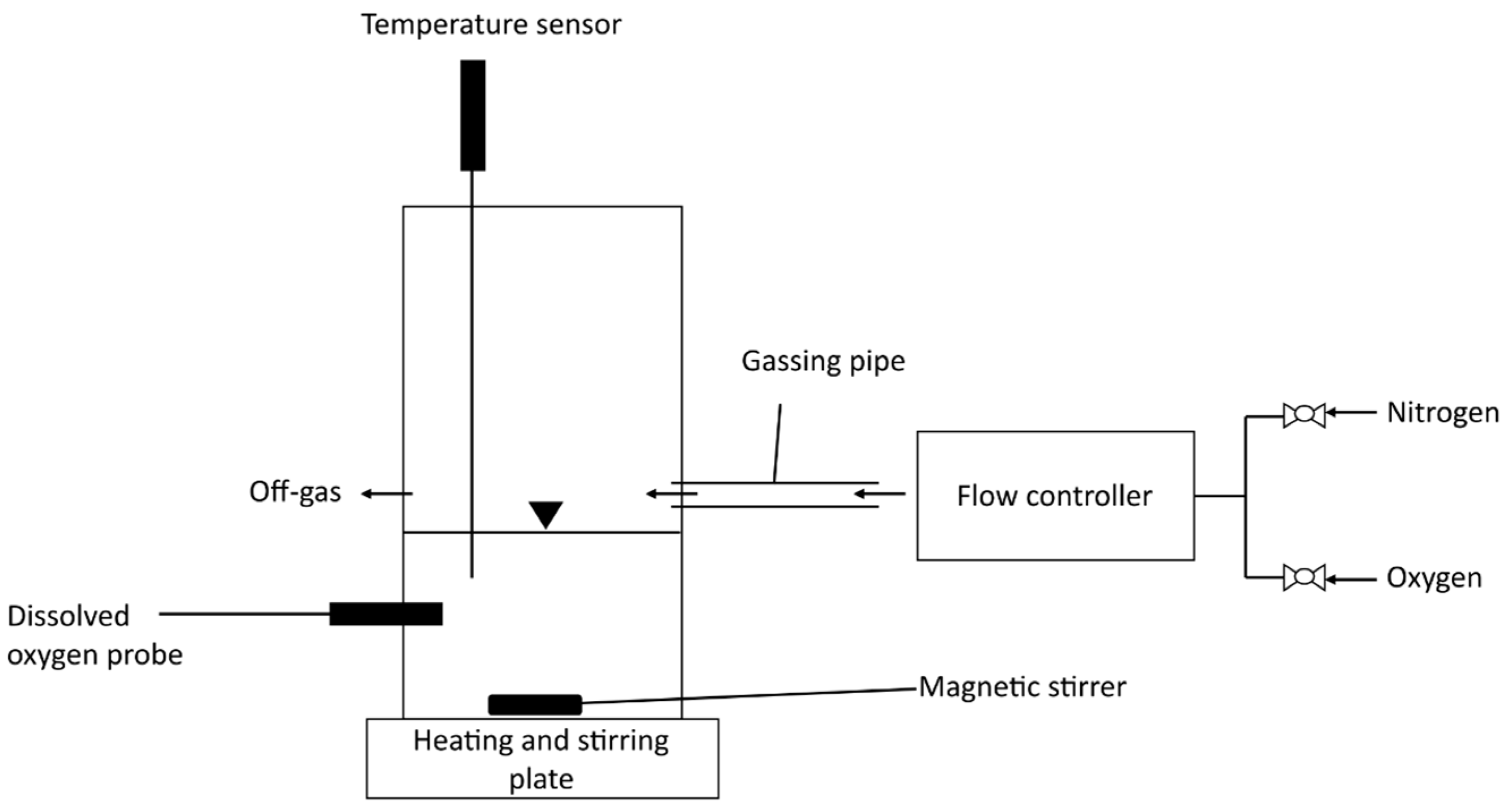
2. Materials and Methods

2.1. Measurement of Diffusion Coefficient

Diffusion coefficients were estimated using a previously described method [28,29]. This approach estimates the volumetric oxygen transfer coefficient kLa at the gas–liquid interface located in the headspace of the reactor. For this purpose, a reaction vessel with a diameter of 3 cm and controlled hydrodynamic conditions was designed, as shown in Figure 1. A liquid phase volume of 35 mL was stirred using a small magnetic stirrer (1 cm) and aerated through a gassing pipe with a diameter of 10 mm. The gassing pipe was located above the liquid surface and aerated with a low gas volume flow of 35 mL min−1. Air flow was controlled using a mass flow controller (Type GSC-B3KA-BB23, Vögtlin Instruments GmbH, Muttenz, Switzerland). The temperature was maintained at 37 °C.
To determine kLa, a dynamic gassing-out technique was applied. Dissolved oxygen concentrations were measured at 30 s intervals using an optical oxygen probe (OXYBase, WR-RS485-A0-L5, PreSens Precision Sensing GmbH, Regensburg, Germany). Because the probe delay of 3 s was small compared with the duration of the experiment (h), no correction was considered. kLa values were estimated by application of (Equation (1)). Logarithmic values were plotted against time. kLa values were obtained from the slope of the linear fit of the respective points.
  ln ( c O 2 , m a x c O 2 c O 2 , m a x c O 2 , m i n ) = k L a × t
From the estimated kLa values, kL was easily obtained by dividing the known specific surface area a, which was calculated by dividing the known liquid volume by the known cross-section of the reactor. According to Hebrard et al. [29], under the conditions of low gas velocities and a flat liquid surface, the gas–liquid mass transfer is mainly controlled by the level of turbulence imposed by the gas flow above the surface. The steps described by Hebrard et al. [29] lead to the following expression for diffusion coefficient D:
D = µ L ρ L × k L C 2 2
The complete derivation of Equation (2), as given by Hebrard et al. [29], is presented in the Appendix A. Material properties µL and ρL were taken from VDI [30]. The constant C2 was determined experimentally at different stirring speeds in deionized water. Using the diffusion coefficient reported by Han et al. [31] for calibration resulted in C 2 = 1.4   ×   10 4   ±   0.6   ×   10 5   m   s 1 as the arithmetic mean and standard deviation of three different measurements. The value of C2 was in the same range as that reported in the literature [28,29].

2.2. Measurement of Oxygen Transfer Coefficient

The experimental kLa values were previously published and thoroughly described by Wild et al. [27]. Briefly, a small bubble column with an inner diameter of 3 cm, and height of 20 cm was used. Gas was sparged through a porous plate with an average pore size of 13 µm. For the determination of kLa, the dynamic gassing-out technique was applied. Nonlinear regression of a first-order approximation considering the influence of the probe response time of 3 s was used to calculate kLa values.

2.3. Measurement of Gas Hold-Up

The experimental data and measurement procedure for gas hold-up were previously published by Wild et al. [27]. The gas content was identified in a transparent tube with the same dimensions as those used for the kLa measurement. The gas hold-up was estimated using a digital imaging technique to compare the liquid levels before and after aeration.

2.4. Measurement of Bubble Size Distribution

The measurement of the bubble size distribution was previously conducted and published by Wild et al. [27]. The tests were performed in a small transparent chamber (length: 250 mm, width: 30 mm, height: 120 mm) which was aerated through a porous plate with an average pore size of 13 µm. A digital imaging technique was used for the estimation. For each bubble size distribution (BSD), at least 110 images, comprising 2500–20,000 bubbles, were analyzed.

2.5. Media Composition

Three different liquids with different amounts of solutes at biologically relevant scales were used: deionized H2O, 1 × phosphate buffer solution (PBS) and minimal medium containing 0.05 % (v/v) antifoam AF (Struktol J647, Schill + Seilacher, Hamburg, Germany) and trace elements. The concentrations of all solubles are shown in Table 1. All chemicals were purchased from Carl Roth GmbH Co. KG (Karlsruhe, Germany).

2.6. Mathematical Model Description
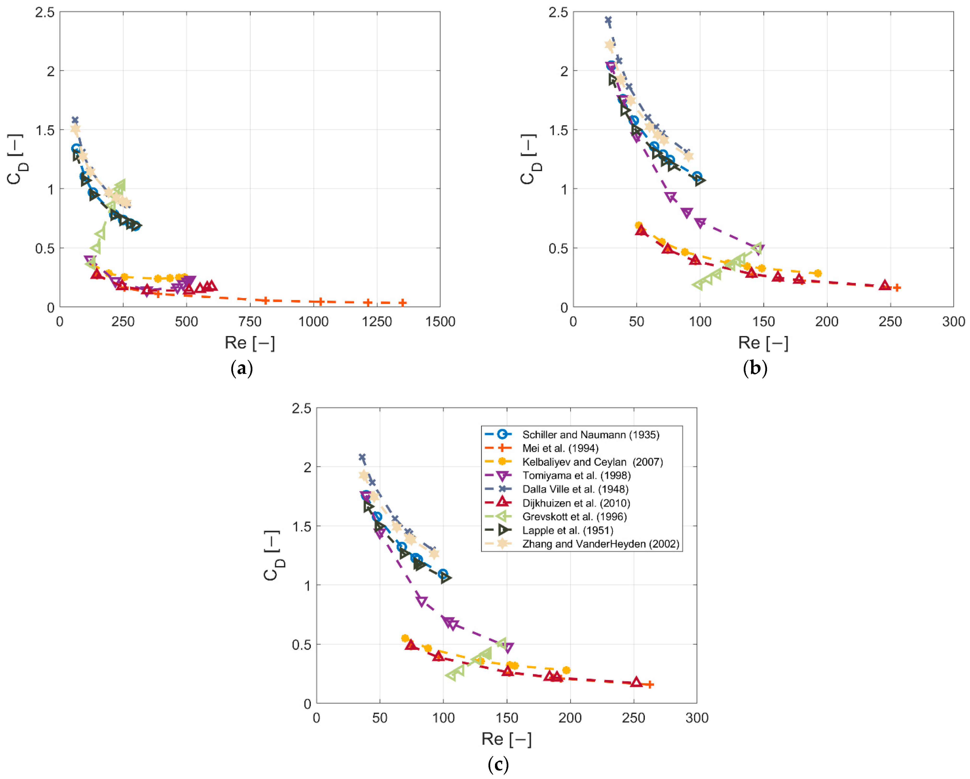
To calculate the rising velocity of the bubbles (uB) and to test different correlations for the drag coefficient (CD) a model was implemented in MATLAB 2022b (MathWorks, Inc., Natick, MA, USA). By formulating the balance of the buoyancy, drag, and gravitation forces exerted on a single bubble, the slip velocity uslip (Equation (3)) was derived:
u s l i p = u B u L = 4 3   g   ρ L ρ G   d 32 ρ L C D
As CD depends on uB in most cases, Equation (3) can only be solved numerically, which was achieved with the Matlab function ‘fsolve’ by applying different models for CD. Further, it was assumed that uL << uB, which means that the influence of the liquid bulk velocity on the terminal bubble rising velocity was negligible (uB = uslip). The feasibility of the simplification was demonstrated by considering and neglecting the comparison uB in the CFD simulations. Nine different correlations for CD (shown in Table 2) were implemented in Equation (3) to derive uB numerically. Therefore, the mean bubble residence time tmean was calculated by Equation (4).
t m e a n = H R u B
This leads to the total gas volume inside the reactor:
V G = t m e a n · V ˙ G
Therefore, the overall gas hold-up α was calculated with V G from Equation (5).
α = V G V G + V L
and the volume-specific surface area a was calculated by Equation (7) after determining α in Equation (6).
a = 6 α d 32   1 α
To calculate the liquid mass transfer coefficient kL, Higbie’s correlation [21]
k L = 2 u s l i p   D O 2 , L π   d 32
and the Frössling approach [20] were considered:
k L =   D O 2 , L   d 32 · 2 + 0.66 R e 0.5 S c 0.33
In any case, the oxygen transfer coefficient kLa was identified as follows:
k L a = k L · a
In the following section, nine different models are presented and used to study their influences on CD. Models that depend on the particle Reynolds number (Re), the Eötvös number (Eo), or both nondimensional numbers are distinguished.
The particle Re is defined as follows:
R e = u B d 32 ρ L   μ L  
For the Eo number holds:
E o = g ρ L ρ G d 32 2   σ  
Table 2. Overview of evaluated drag models.
Models based on Re
Schiller and Naumann [12] C D = 24 R e   1 + 0.15   R e 0.687   ,     R e < 1000 0.44 ,       R e 1000   (13)
Dalla Valle [32] C D = 0.63   4.8 R e 2 (14)
Lapple [33] C D = 24 R e   1 + 0.125   R e 0.72 ,     R e   1000 (15)
Mei and Klausner [34] C D = 16 R e   1 + 8 R e + 0.5   1 + 3.315   R e 0.5 1 ,       0.1 < R e < 200 (16)
Zhang and van der Heyden [35] C D = 0.44 + 24 R e + 6 1 + R e (17)
Models based on Eo
Grevskott et al. [36] C D = 5.645 E o 1 + 2.835 (18)
Models based on both Re and Eo
Tomiyama [10] (pure water) C D = m a x min 16 R e   1 + 0.15   R e 0.687 ,   48 R e ,   8   E o 3   E o + 4 (19)
Tomiyama [10] (slightly contaminated water) C D = m a x min 24 R e   1 + 0.15   R e 0.687 ,   72 R e ,   8   E o 3   E o + 4 (20)
Tomiyama [10] (fully contaminated water) C D = m a x 24 Re   1 + 0.15   R e 0.687 ,   8   E o   3   E o + 4 (21)
Kelbaliyev and Ceylan [37] C D = 16 R e   1 + R e 1.385 12 1 55 + 8 3   R e 4 3   M o 1 3 24   1 + M o 1 3 + R e 4 3   M o 1 3 ,     0.1     R e < 0.5   8 R e   1 + 1 1 0.5   1 + 250   R e 5 2 ,   0.5     R e     100 (22)
The Morton (Mo) number is defined as follows:
M o = g ρ L ρ G   µ L 4   ρ L 2 σ 2   (23)
Dijkhuizen et al. [11] C D = C D , M e i 2 + C D E o 2 0.5 (24)
C D , M e i = 16 R e   1 + 8 R e + 0.5   1 + 3.315 R e 1 (25)
C D E o = 4   E o E o + 9.5 (26)

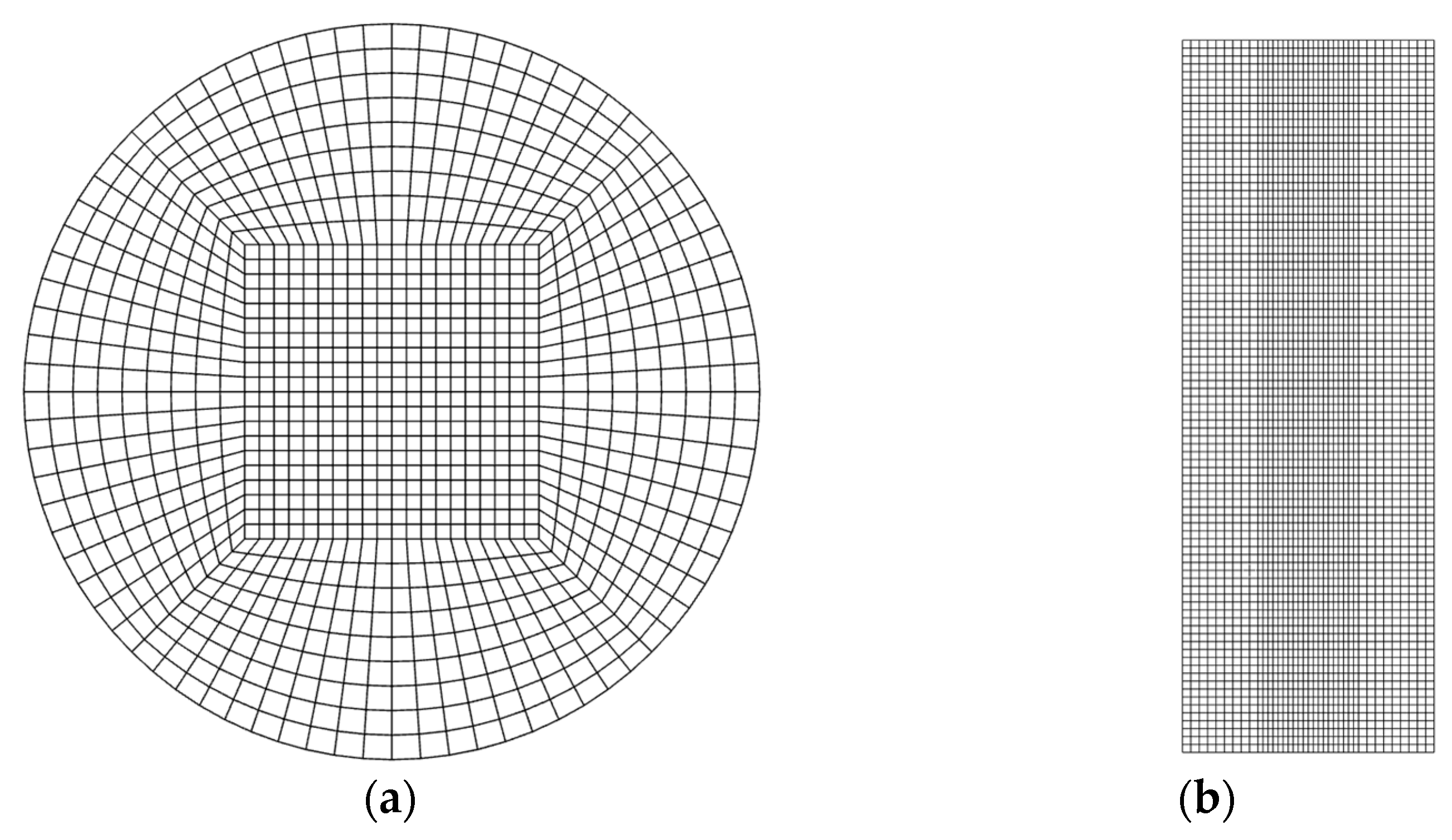
2.7. Computer Fluid Dynamic Simulation Set-Up

The CFD simulation was conducted using the commercial software ANSYS Fluent 2019. The Reynolds-averaged Navier–Stokes equations (RANS) combined with the RNG (renormalization Group) k-ε-model were solved with the help of a finite volume (FV) framework. Numerous simulation studies have been conducted to investigate laboratory-scale bubble columns using Euler–Euler approaches combined with the k- ε model [2,38,39,40].
The underlying Euler–Euler approach treats interacting phases by assuming that each phase behaves as an interpenetrating continuum. The geometry and experimental settings are similar to those used by Wild et al. [27]. The bubble column was cylindrical, with a height of 85 mm, a diameter of 30 mm, and a total volume of 60 mL. The cross-sectional area of the bed plate was used for aeration. The superficial gas velocity varied between 0.12 and 0.59 cm s−1 for the air inlet as a mixture of CO2, N2, and O2. The measured BSD was categorized into 20 evenly distributed classes at the inlet.
The boundaries of the smallest and largest size classes were defined as the lowest and largest bubble diameters, respectively. An overview of the size ranges is provided in Appendix B. Bubble breakage and coalescence models were not considered. The gas phase exited the column at the top with a degassing outlet boundary, whereas the sidewalls were defined under no-slip conditions. In addition to the drag coefficient, no additional bubble forces were applied. The volume was discretized using a 100, 800-hexahedron mesh, resulting in a density of 1680 elements m L−1. In a similar investigation, the mesh used by Rampure et al. [41] was significantly coarser. An investigation of grid independence was conducted, and the outcomes concerning the integrated gas content are presented in Appendix C.
Using a constant time step of 1 ms, a convergence criterion of 10−4 (usually significant lower) for all residuals was reached after a maximum of 45 iterations. The spatial discretization of the convective term was set to a high-order QUICK scheme for the velocities [42]. Pressure and velocity were coupled via the “Phase Coupled SIMPLEC” algorithm [43]. Pseudo-steady-state conditions were achieved when the gas flow rates converged at the outlet. The simulations were then stopped, typically after 2–8 s. Appendix C shows that the gas hold-up remained constant in the pseudo-steady state. At low gas hold-up levels, where the bubble swarm effects were negligible, it was possible to characterize the values using a non-transient method.

3. Results and Discussion

3.1. Identification of Diffusion Coefficients in Aqueous Solutions

The diffusion coefficients DA,M are physical constants that characterize the concentration-driven mass transfer of component A in the surrounding matrix M. Here, the oxygen-to-liquid mass transfer was investigated (A = O2, M = aqueous solution), which may be affected by soluble compounds [44] and temperature [31]. For simplicity, the related diffusion coefficient was termed D. Although a priori knowledge of D is a desirable, commonly accepted approach to correctly predict diffusion constants, it has yet to be confirmed [28]. Therefore, D was experimentally determined before applying it to Higbie’s mass transfer model. As indicated in Table 3, the addition of solutes decreased D values, which agrees with reported observations [29,44,45]. The magnitude of this reduction was similar to that reported by Jamnongwong et al. [28], who investigated the effects of glucose and NaCl solutions on the diffusion. D was derived from Equation (2) and depended on the kLa estimation, which was the source of the deviations between the measurements.

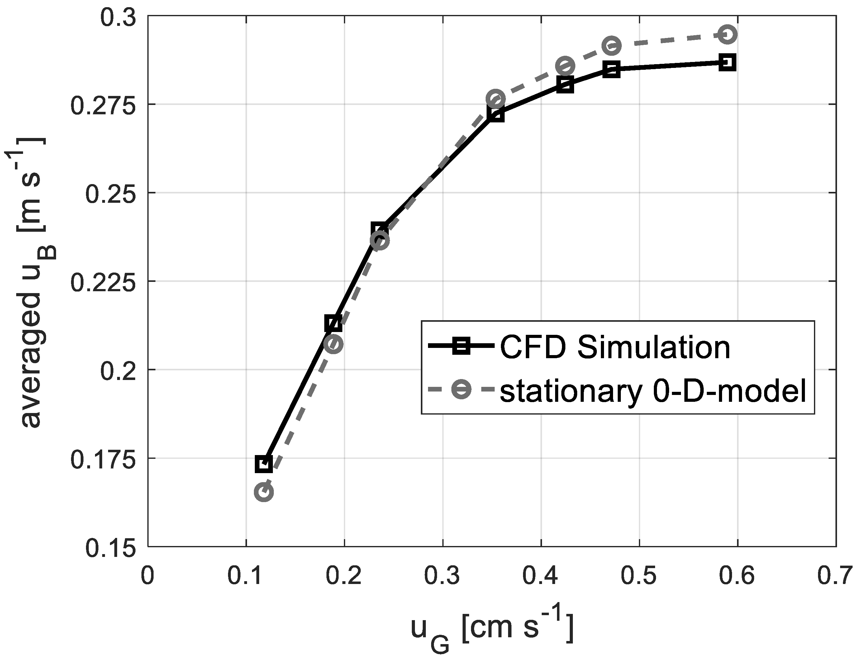
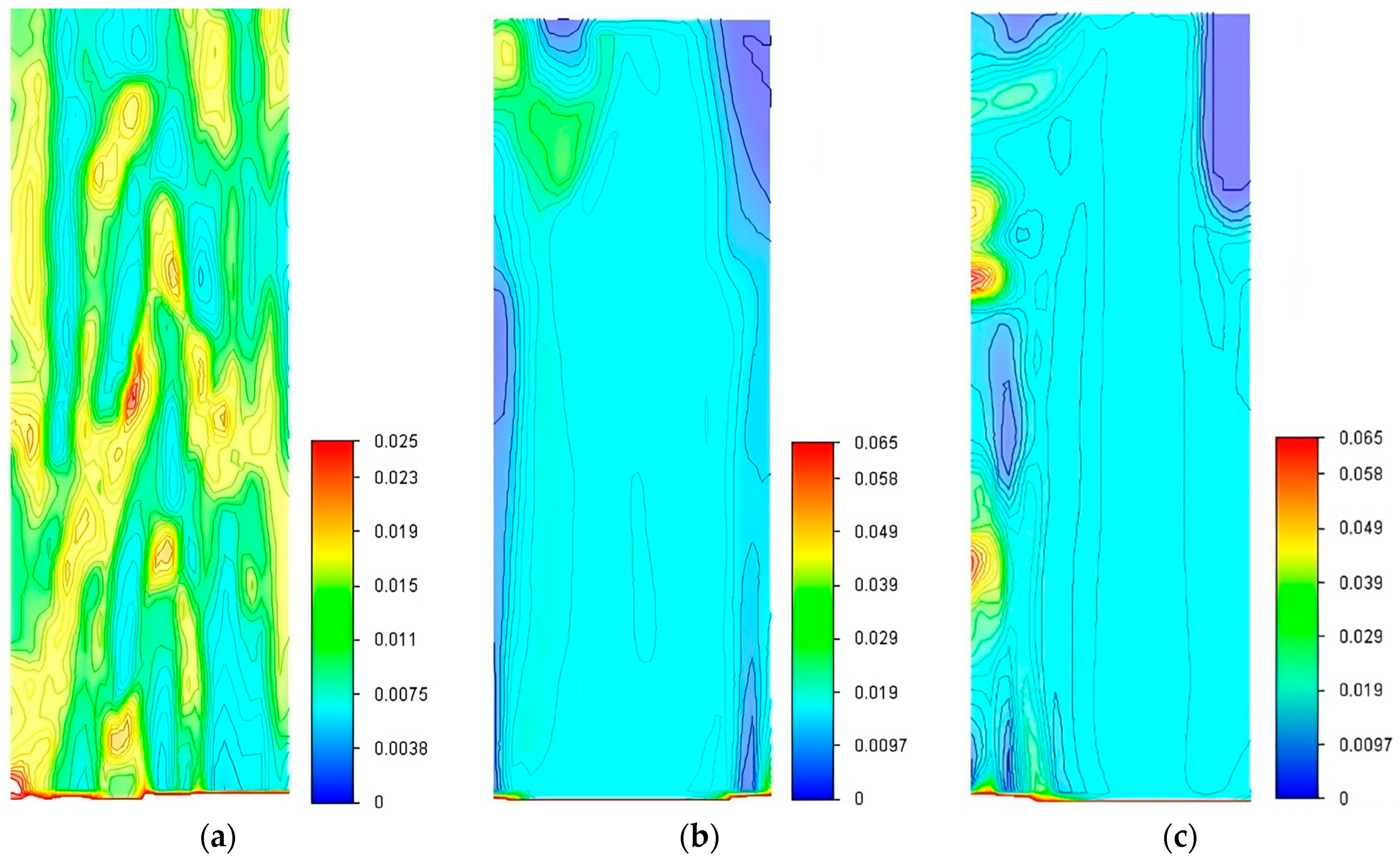
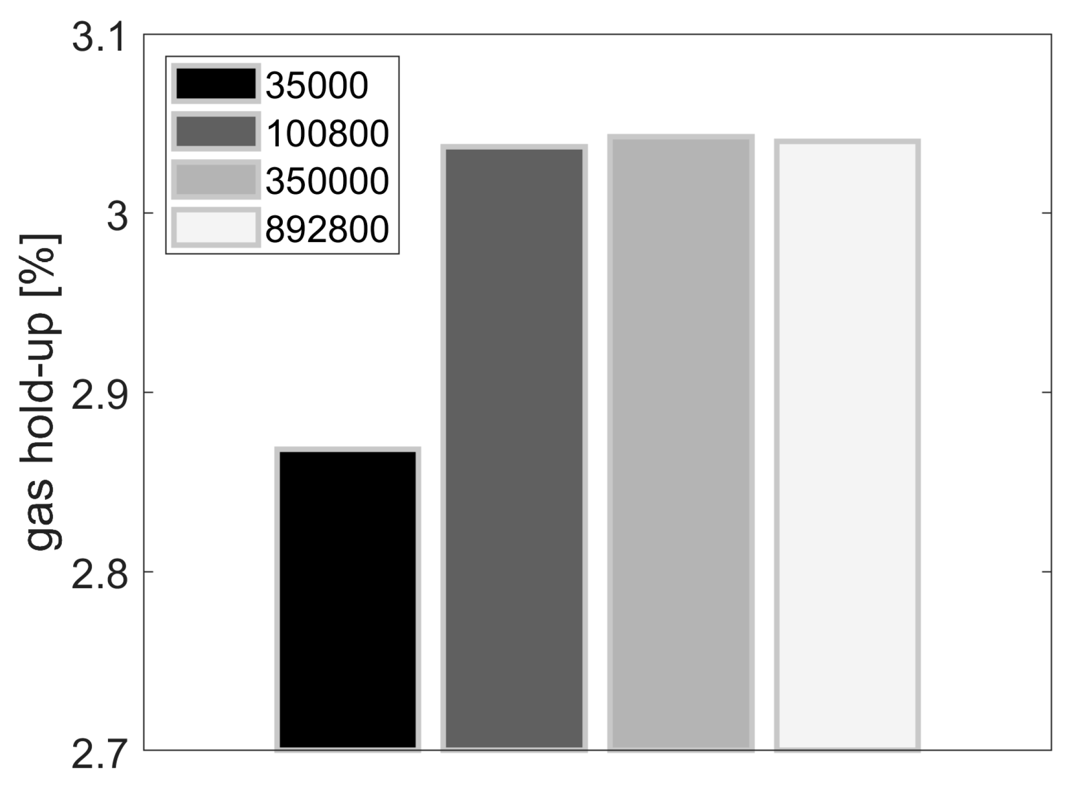
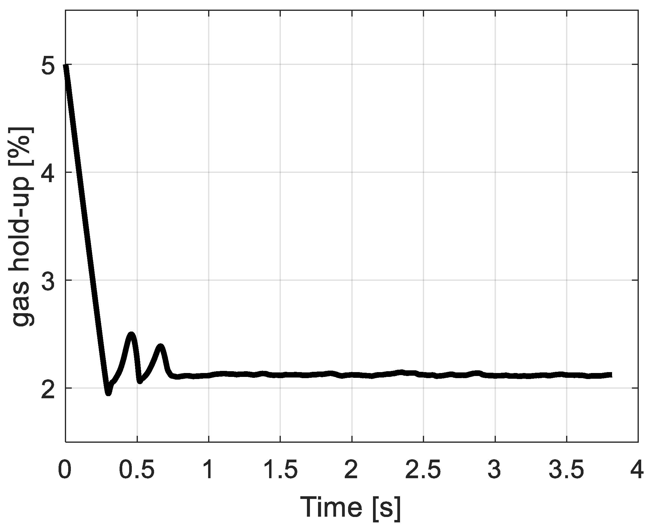
3.2. CFD Simulations

Figure 2 shows the resulting average bubble ascent velocities from the numerical MATLAB solution compared with the CFD results. Notably, CFD calculated uB based on the solved fluid field, including the impact of fluid motion. In contrast, the MATLAB prediction was a simplified stationary approach that ignored the spatial resolution and fluid movement. Irrespective of these simplifications, the velocity predictions were similar.
At uG 0.12 cm s−1, the gas hold-up deviated to a maximum of 4.55% and decreased to a deviation of 2.74% at uG 0.59 cm s−1. In both approaches, the drag model was implemented according to Kelbaliyev et al. [37]. The combination of a low gas hold-up and small bubbles ensured that only slight fluid movement was induced. As shown in Figure 2, even for the highest uG of 0.59 cm s−1, the ascent bubble velocity was 28.0 cm s−1 while the mean fluid velocity was still only 0.86 cm s−1. Therefore, it can be concluded that neglecting the bubble–liquid and bubble–bubble interactions in the simplified MATLAB approach is acceptable for low gas hold-ups.
Figure 3 shows the gas distribution in the bubble column for deionized water, PBS, and minimal medium. The contour plane was located at the center of the column and spanned the height from the inlet to the outlet. The profiles of PBS and minimal medium were similar, with d32 values of 0.79 and 0.80 mm, respectively. Consequently, the gas was evenly distributed across the column’s width. In PBS, the gas gradients were difficult to identify. The gas, rarefied as a liquid. flowed downwards only at the outer edges. With respect to the minimal medium, there were some spots on the reactor wall indicating increased gas density caused by aggregating bubbles. This mimics the common observation that a down-coming liquid may initiate bubble accumulation at the reactor walls. Sangani et al. [46] demonstrated that these bubble-swarm effects can be explained by the occurrence of viscous forces. Because there was no liquid movement between the aggregated bubbles, the local pressure was smaller than that outside the agglomerate, which finally led to bubble aggregation. This effect became more pronounced the larger d32 was. Consequently, bubble swarms were observed more frequently in deionized water, because d32 was 1.52 mm. Characteristic microstructures with an undefined liquid reflux were formed.

3.3. Correlation of the Drag Coefficient with Re Number

Figure 4 shows the dependence of CD at different Re numbers. The Re numbers were computed using the Sauter diameters obtained from the experiments conducted by Wild et al. [27] and can be seen in Appendix B. The ascent velocity of the bubbles was determined by the drag coefficient which was employed, making the Re number a variable dependent on CD. For small Re values, the flow was laminar, and CD decreased proportionally with Re. For a higher Re, the flow may have remained laminar; however, the effects of turbulence became more significant. The drag coefficient still decreased with increasing Re, but the rate of the decrease was generally slower than that in the very low Re regime. The Re numbers shown for PBS and minimal medium exhibited a peak of approximately 250, whereas deionized water produced values of approximately 500. These observations are consistent with the findings of Wild et al. [27], who indicated that the bubble diameters in PBS and minimal medium were smaller than those observed in water. The model proposed by Mei et al. [47] rendered a smaller drag coefficient, resulting in much higher bubble velocities, leading to a Re of up to 1350 for deionized water. Substantial differences appeared between the various drag models, resulting in CD values that differed by a factor of approximately three for water at low Re values exceeding 1. In the case of PBS and minimal medium, these differences were even more significant, with CD values surpassing 1.5. The CD values calculated according to Grevskott et al. [36] increased linearly with Re because they depend only on the Eo number.

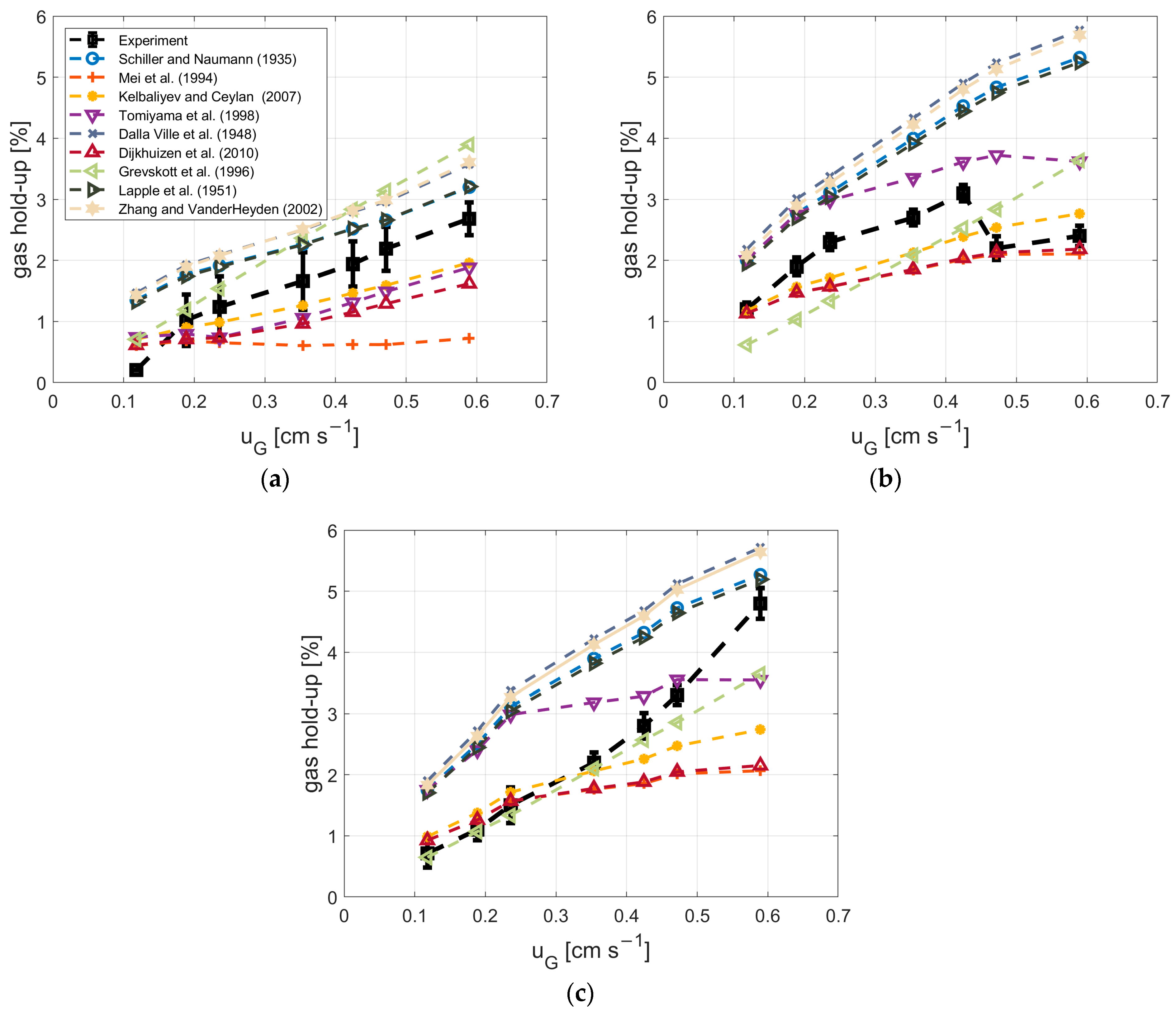
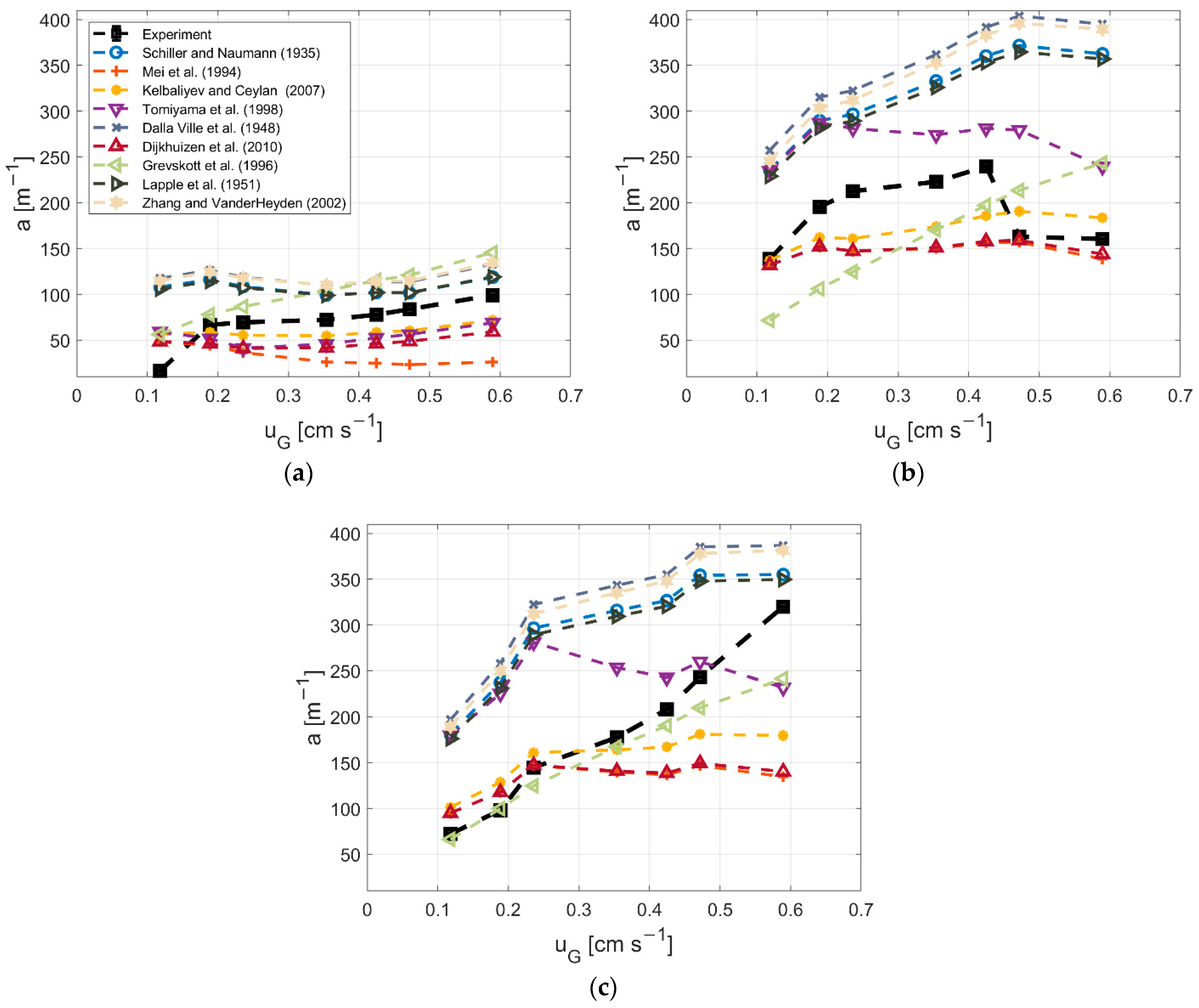
3.4. Dependency of Gas Hold-Up and a on the Drag Model

According to the experiments of Wild et al. [27], based on fundamental insights into the bubble size and resting times, it was possible to perform a comprehensive analysis of various drag models. Wild et al. [27] employed a digital imaging technique to measure the resulting bubble size distributions and gas hold-ups. These measurements allowed for the calculation of the volume-specific surface area. Furthermore, a dynamic gassing-out technique was used to determine the kLa value. These experimental procedures were performed for various types of liquids using the geometry described above.
Drag models can be classified into two categories: those that depend only on Re and those that additionally include the Eo number. The Eo number, which represents the ratio between the gravitational force and surface tension, governs the motion of the bubbles. As the bubbles flattened, the Eo number increased, leading to a corresponding increase in CD values [48]. The model proposed by Grevskott et al. [36] is the only one that depends exclusively on Eo.
According to Wild et al. [27], an increase in uG produces larger bubbles. Consequently, the gas hold-up and bubble ascent velocities increased, causing shortened residence times. The correlation between the gas hold-up and uG is outlined in Figure 5. Almost all models revealed a positive correlation, leading to a continuous increase in the gas hold-up with increasing uG. As the Eo number solely follows d32 and does not depend on uB, the models of [10,11,36] revealed different trends. The approach of Tomiyama et al. [10] is probably the most commonly applied drag force model. Notably, the model relies on the Eo number and distinguishes between clean, slightly contaminated, and fully contaminated liquid phases, as shown in Equations (19)–(21). This finding is consistent with those of Nalajala et al. [49], who reported that the flow separation at the bubbles differs significantly between contaminated and clean fluids because surfactants manipulate the shape and surface mobility of the bubbles. Supporting observations reported by Tzounakos et al. [50] show that the ascent velocity decreased with increasing surfactant concentration. Figure 5b,c reflect the anticipated effects of the surfactants on the gas hold-up. Considering the model proposed by Tomijama et al. [10], the deionized water approach (Equation (19)) best fits Figure 5b, whereas Equation (20) has superior predictability for PBS and minimal media (Figure 5b,c). However, none properly mirrored the experimental findings. In the associated study conducted by Wild et al. [27], the diameter range of d32 for water was found to be between 0.76 and 1.67 mm, while for PBS and medium, the range was narrower, ranging from 0.52 to 0.94 mm. The different gas hold-up levels are, therefore, mainly due to the dependence of CD on d32, while the consideration of contaminated fluid only leads to a minor improvement and may also be neglected.
The models reported by [12,32,33,35] showed similar trends, but differed slightly in their choices of empirical constants. Notably, they relied only on the Re number and consistently overestimated the experimentally determined gas hold-up. After reaching a certain threshold of Re, vortices were formed at the tear-off flow of the bubble, which led to an increase in the form resistance of the bubble, and the influence of the viscous stress became minor [14]. The models were adapted from Stokes’ law, which is formulated for very small Re numbers. To extend these solutions to higher Re numbers, correction factors were included in the models, which led to a nonlinear relationship between the Re number and drag coefficient. In our study, the Re values were in the range of 10–500, indicating that the system approached the transition from the viscous stress regime to the turbulent tear-off condition. However, for small bubbles, a spherical shape could be assumed even at higher Re numbers because the capillary pressure was very high. By considering the Eo number (significantly smaller than 1), the spherical shape was characterized despite high Re numbers, and the models of [10,36] showed better agreement with the experimental results than the other expressions. The results demonstrated that applying different correlations to the drag coefficients can significantly affect the predicted gas hold-up.
The drag coefficient of Mei et al. [47] underrated the gas hold-up of deionized water, PBS, and minimal medium. Notably, the follow-up approach of Dijkhuizen et al. [11] underestimated the real gas hold-ups for PBS and minimal medium, particularly when Re values were larger than 10. However, the Eo correction proposed by Dijkhuizen et al. [11] improved the predictions for deionized water (Figure 5).
The rapid ascent of small bubbles in the column resulted in Re numbers exceeding 200. However, owing to the prevalence of high capillary forces associated with small diameters, these bubbles retained their spherical shape and exhibited stabilizing effects. Consequently, they induced minimal back turbulence. In such cases, the viscous force dominates the bubble rise, which motivates the additional consideration of the Morton (Mo) number (Equation (23)). The dimensionless criterion represents the ratio of the viscous forces to the surface tension, which is independent of the bubble’s diameter. The drag model proposed by Kelbaliyev et al. [37] is the only one that includes the Mo number, and, notably, this approach provided the best predictions for all uG values of the three liquids. For small Re values, the gas hold-up deviated only slightly from the experimentally determined values. According to a study by Kelbaliyev et al. [37], the deformation of the bubbles starts beyond the threshold of Re · Mo1/6 > 7. As the Mo number remained at 2.6 × 10⁻¹¹ and Re values did not exceed 500, the criterion for bubble deformation was not achieved. Hence, the model correctly predicted the existence of spherical bubbles and did not include the influence of back turbulence on the drag coefficient. The other models did not determine the Stokes assumption for this Re range or adjust the drag coefficient accordingly. For the specific case of small spherical bubbles, this generates inaccuracy [14].
Comparing Figure 5 and Figure 6, only the models that effectively predicted the gas hold-up also exhibited high degrees of agreement in their predictions of a. Nonetheless, substantial disparities are evident among certain models and experimental findings concerning a. As the aeration rate increased, the gas hold-up approached 1, resulting in a stronger dependence on d32 in Equation (7). Nevertheless, within the examined range of α up to 6%, the impact of gas hold-up and d32 counterbalanced each other for a. With increasing uG, a was identified as stable, with only slightly increasing values. For example, Grevskott et al. [36] identified the only drag coefficient that predicts a continuous increase in a for higher uG. For PBS and minimal medium, this model reproduced the experimental results well. However, the simulated a increasingly deviated from the experimental values for deionized water. As in the case of gas hold-up, Kelbaliyev et al. [37] yielded the best results as a universal model for all liquids and superficial gas velocities. The models proposed by Tomijama et al. [10] overestimated a for PBS and minimal medium. The models of [12,32,33,35] correctly reflected this trend; however, a was significantly overestimated. Drag coefficients obtained by Mei et al. [48] and Dijkhuizen et al. [11] underestimated a, particularly for deionized water and the minimal medium.

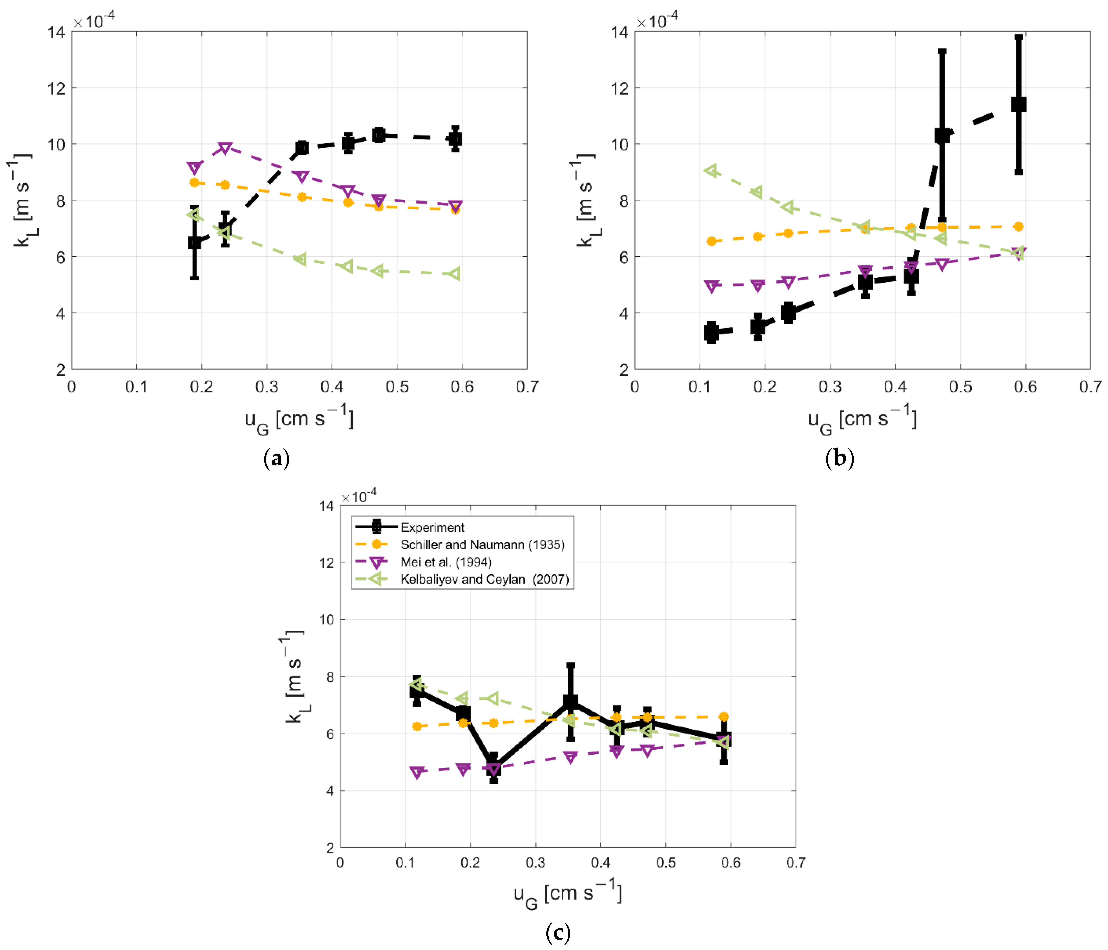
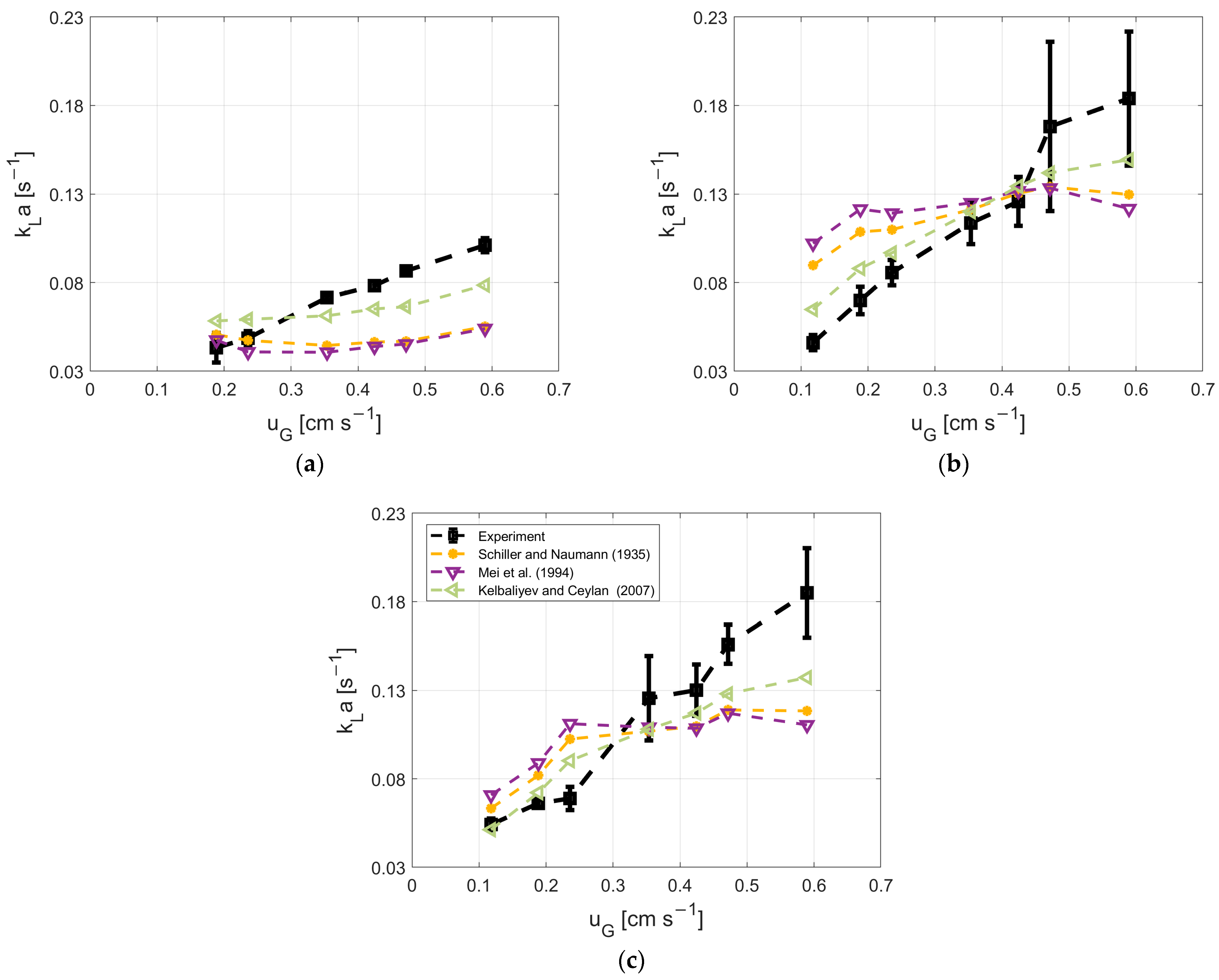
3.5. Model Description for kL and kLa

To estimate the mass transfer coefficient kL, the results of the three best-fitting drag models were selected. Using the steady-state bubble velocity, uB and kL were obtained using the Higbie approach in Equation (8). As shown in Figure 7, the simulated values were similar to previously published experimental values [27]. In general, kL decreased with increasing superficial gas velocity. This may reflect the impact of growing bubble diameters resulting from increased uG [27], which was also observed experimentally [51,52]. For example, Grevskott et al. [36] continued this trend for PBS and minimal medium. In contrast, Kelbaliyev et al. [37] and Tomiyama et al. [10] inverted the course, leading to rising kL with increasing uG in PBS and minimal medium. This phenomenon may be explained by the different trends of the bubbles’ rising velocities calculated using different drag models. Irrespective of the drag model, the resulting ascent velocity, uB, determined kL. The predicted kL increased only if uB increased at a faster rate than d32.
A comparison of the simulated data with the experiments revealed opposite trends, particularly for deionized water and PBS. Whereas for low superficial gas velocities, the experimental values were smaller than the predicted values, and the inverse occurred for large uG. This might reflect the occurrence of different mass-transfer regimes, as suggested by [52,53]. The two regimes were distinguished by their mass transfer rates and bubble sizes. The threshold bubble diameter defines the transition from low to high kL, and vice versa. This transition phenomenon may explain the experimentally observed kL dynamics; however, it was not implemented in any of the drag models used. As the crucial input value, uB relies intrinsically on the drag model in Equation (3) This correlation challenges the suitability of the Higbie approach. Nevertheless, the assumption of a mobile bubble surface, for which the values may be predicted using Higbie’s equation by Alves et al. [54], seems to be justified, as it predicts values in the same range as the experimental data, whereas the application of Frössling’s mass-transfer correlation predicted values that were ten-fold lower.
The mass transfer coefficients kLa combine a and kL and are depicted in Figure 8. For all liquids, the models captured the basic trend of increasing kLa with increasing uG. However, the dynamics were not fully reflected in deionized water, PBS, or minimal medium at high uG. The reasons for this are shown in Figure 6 and Figure 7, indicating that a and kL are underestimated for these regimes. This analysis outlines the need to choose the proper drag model to achieve acceptable mass transfer predictions.

4. Conclusions

In addition to their significant potential for parallelizing and automating microbial strain testing, small-scale bubble columns are suitable for studying the distinct effects of drag forces in a well-defined manner. The fluid was characterized by a low gas hold-up and equally distributed spherical bubbles, owing to their small diameters. Hence, the device parameters of BSD, kLa, and gas hold-up are easy to detect, and the bubble swarms and bubble-to-bubble interactions have minimal influence. The choice of a compatible drag coefficient strongly affects the hydrodynamics of the fluid and has a far-reaching influence on the phase–mass exchange rate when simulating multiphase reactors. These effects were sufficiently substantial to overcome the contributions of the other bubble forces. Moreover, in small-scale systems, the influence of wall effects on the resulting drag forces is substantial. Therefore, a suitable drag model that accounts for the prevailing dimensional numbers must be determined with the utmost caution. The most effective performance was obtained by investigating not only Re, but also Mo and Eo.
The liquid mass transfer description of Higbie is justifiably one of the most widespread models, as it outperforms the results of other approaches, such as Frössling. Moreover, the knowledge of properly identified liquid diffusion coefficients is important for improving mass-transfer predictions. This finding holds particularly true for fermentation conditions characterized by media with physical properties that differ from those of water. The analysis via stationary 0-D mechanistic models is a fast, straightforward implementation that facilitates the selection of the best-suitable drag model. Multiphase systems with bubble sizes smaller than 1.5 mm enabled the highest mass transfer and mixing performances. Furthermore, they facilitated modeling owing to their spherical bubble characteristics. Accordingly, such small-diameter bubble systems are likely to gain momentum in future applications. Identifying the influence of wall effects and alternative drag models that can best cope with such fermentation conditions is a promising task for future applications.

Author Contributions

Conceptualization, Y.M., M.W. and R.T.; formal analysis, Y.M. and M.W.; funding acquisition, R.T.; investigation, Y.M. and M.W.; methodology, Y.M. and M.W.; project administration, R.T.; resources, R.T.; software, Y.M. and M.W.; supervision, R.T.; validation, Y.M. and M.W.; visualization, Y.M. and M.W.; writing—original draft, Y.M. and M.W.; writing—review and editing, Y.M., M.W. and R.T. All authors have read and agreed to the published version of the manuscript.

Funding

This research received no external funding.

Data Availability Statement

Data are contained within the article.

Conflicts of Interest

The authors declare no conflicts of interest.

Nomenclature

avolume-specific surface aream−1
CDdrag coefficient-
c O 2 oxygen concentration in liquidmmol L−1
D O 2 , L diffusion coefficient of oxygen in liquid phasem2 s−1
d32Sauter mean diameterm
fiinternal friction factor-
ggravity constantm s−2
HRreactor heightm
kLavolumetric oxygen transfer coefficients−1
kLmass transfer coefficientkg m−1 s−1
srenewal rate of liquid elements at the gas–liquid interfaces−1
ttimes
tmeanmean residence times
Uiinterfacial momentum transfer velocitym s−1
uGgas velocitym s−1
uLliquid velocitym s−1
uBaveraged bubble rising velocitym s−1
VGvolume of the gas phasem3
VLvolume of the liquid phasem3
V ˙ G volume flow rate airm3 s−1
Greek Symbols
α gas hold-up-
Εcharacteristic scales of velocity and lengths−1
ν kinematic viscosity of the liquid phasem2 s−1
µLdynamic viscosity of the liquid phasem2 s−1
ρLdensity of the liquid phasekg m−3
ρGdensity of the gas phasekg m−3
σ surface tensionkg s−2
τiinterfacial momentum transfer stresskg m−1 s−2
Abbreviations
AFantifoam
BSD bubble size distribution
CFDcomputational fluid dynamics
EoEötvös number
MM minimal medium
MoMorton number
PBSphosphate buffer solution
ReReynolds number
ScSchmidt number
0-Dzero-dimension

Appendix A

The derivation of the equation used to estimate the diffusion coefficients was based on the derivation given by Hebrard et al. [29]. Accordingly, under conditions of a low gas velocity UG and a flat liquid surface with a very low liquid velocity UL, the gas–liquid mass transfer is mainly controlled by the level of turbulence imposed by the gas flow above the surface. The interfacial momentum transfer stress τi can then be expressed as
τ i = 1 2 × ρ G × f i × U G U L 2
where fi denotes the interfacial friction factor. The interfacial momentum transfer velocity is then defined as
U i * = τ i ρ l
in Danckwerts et al. [22] It was proposed to model the liquid mass transfer coefficient based on the renewal rate of liquid elements at the gas–liquid interface with respect to
k L = D × s
where D is the diffusion coefficient of the solute in the liquid phase. The latter parameter, s’, for a free interface sheared by a gas flow was expressed by Fortescue et al. [55] as
s = C 3 × ϵ
with C3 as a constant and ϵ as ratio between the characteristic scales of velocity and length. The interfacial shear stress was linked to the viscosity by the following equation:
μ L = τ i ϵ
By combining Equations (A1)–(A5), kL could be expressed as
k L = D × C 3 × τ i μ L
With the introduction of the Schmidt number Sc into Equations (A7) and (A2), the model proposed by Danckwerts et al. [22] became
k L U i * × S c 0.5 = C 1
This is the general form of the correlation related to the absorption coefficients. The power of the Schmidt number depends on the nature of the interfaces; for solid boundaries, it is equal to 2/3 instead of 1/2 in the present case. In the experiments, low gas flows and agitation rates were constantly imposed. It was, therefore, assumed that the interfacial momentum transfer stress τi, and thus the associated velocity U i * , remained constant for similar phase properties. Under these conditions, the diffusion coefficient, D, in the liquid phase could be expressed as
D = μ L ρ L k L C 1 U i * 2 = µ L ρ L k L C 2 2
where the constant C2 is defined as the product of the constant C1 and the interfacial momentum transfer velocity U i * . With a known mass transfer coefficient kL from the measurement, known liquid phase properties, and an estimation of the constant C2, the diffusion coefficient could be calculated using Equation (A8).

Appendix B

Table A1. Upper and lower limits for the bubble size distribution and the respective Sauter diameter for each of the measured superficial gas velocities.
uG in cm s−1 d min in mm d max in mm d32 in mm
0.120.162.970.76
0.190.163.510.93
0.240.163.881.08
0.350.163.881.40
0.420.153.881.52
0.470.154.031.61
0.590.154.091.67
For the CFD simulation of a small-scale bubble column, the inlet bubble size distribution corresponding to the respective superficial gas velocity was selected based on the experimental measurements of Wild et al. [27]. The BSD was part of a (PBM) and comprised 20 uniformly distributed size classes for the bubble diameter. The bubble diameter range was redefined based on the measured diameter scale of the bubbles. The starting and ending values of this distribution can be found in Table A1 for each superficial gas velocity.

Appendix C

Figure A1. Mesh for bubble column simulation in Ansys Fluent. (a): View from the top; (b): section view from the side.
Processes 12 00045 g0a1
The mesh for the CFD simulation of the column consisted of 100,800 hexahedrons with inner rectangular sections and uniform grid cells. The minimum orthogonal quality was 0.76. Compared to the coarse mesh of the medium one, the calculated gas hold-up was 6% higher. If the mesh were further refined to 350,000 cells, the value would deviate by only 0.002%. Therefore, it can be assumed that a mesh density of 100,800 is sufficient to accurately represent the fluid motion.
Figure A2. Mesh independence study with 3 different mesh densities. The gas hold-up in the column after reaching a pseudo-steady state at a uG of 0.59 cm s−1.
Processes 12 00045 g0a2
Figure A3. The gas hold-up progression over time is depicted for the simulation of the small-scale bubble column, starting from an initial value of 5%. The superficial gas velocity was set to 0.59 cm s−1.
Processes 12 00045 g0a3
Considering the small volume of the column and low gas volume flow, it was expected that pseudo-equilibrium would be reached within a very short time. Figure A3 shows that this became apparent after less than 1 s, indicating that the residence time of the bubbles was very short. Subsequently, it is evident that the gas inflow and outflow were in equilibrium, and the gas hold-up remained relatively constant.

References

  1. Ngu, V.; Morchain, J.; Cockx, A. Spatio-temporal 1D gas–liquid model for biological methanation in lab scale and industrial bubble column. Chem. Eng. Sci. 2022, 251, 117478. [Google Scholar] [CrossRef]
  2. Frey, L.J.; Vorländer, D.; Ostsieker, H.; Rasch, D.; Lohse, J.-L.; Breitfeld, M.; Grosch, J.-H.; Wehinger, G.D.; Bahnemann, J.; Krull, R. 3D-printed micro bubble column reactor with integrated microsensors for biotechnological applications: From design to evaluation. Sci. Rep. 2021, 11, 7276. [Google Scholar] [CrossRef] [PubMed]
  3. Siebler, F.; Lapin, A.; Takors, R. Synergistically applying 1-D modeling and CFD for designing industrial scale bubble column syngas bioreactors. Eng. Life Sci. 2020, 20, 239–251. [Google Scholar] [CrossRef] [PubMed]
  4. Siebler, F.; Lapin, A.; Hermann, M.; Takors, R. The impact of CO gradients on C. ljungdahlii in a 125 m3 bubble column: Mass transfer, circulation time and lifeline analysis. Chem. Eng. Sci. 2019, 207, 410–423. [Google Scholar] [CrossRef]
  5. Gradov, D.V.; Laari, A.; Turunen, I.; Koiranen, T. Experimentally validated CFD model for gas–liquid flow in a round-bottom stirred tank equipped with Rushton turbine. Int. J. Chem. React. Eng. 2017, 15, 20150215. [Google Scholar] [CrossRef]
  6. Lou, W.; Zhu, M. Numerical simulation of gas and liquid two-phase flow in gas-stirred systems based on Euler–Euler approach. Metall. Mater. Trans. B 2013, 44, 1251–1263. [Google Scholar] [CrossRef]
  7. Ruthiya, K.C.; van der Schaaf, J.; Kuster, B.F.M.; Schouten, J.C. Influence of particles and electrolyte on gas hold-up and mass transfer in a slurry bubble column. Int. J. Chem. React. Eng. 2006, 4. [Google Scholar] [CrossRef]
  8. Hikita, H.; Asai, S.; Tanigawa, K.; Segawa, K.; Kitao, M. Gas hold-up in bubble columns. Chem. Eng. J. 1980, 20, 59–67. [Google Scholar] [CrossRef]
  9. Kellermann, H.; Jüttner, K.; Kreysa, G. Dynamic modelling of gas hold-up in different electrolyte systems. J. Appl. Electrochem. 1998, 28, 311–319. [Google Scholar] [CrossRef]
  10. Tomiyama, A.; Kataoka, I.; Zun, I.; Sakaguchi, T. Drag coefficients of single bubbles under normal and micro gravity conditions. JSME Int. J. Ser. B 1998, 41, 472–479. [Google Scholar] [CrossRef]
  11. Dijkhuizen, W.; Roghair, I.; van Sint Annaland, M.; Kuipers, J. DNS of gas bubbles behaviour using an improved 3D front tracking model—Drag force on isolated bubbles and comparison with experiments. Chem. Eng. Sci. 2010, 65, 1415–1426. [Google Scholar] [CrossRef]
  12. Schiller, L.; Naumann, A.; Drag, A. Coefficient Correlation. Z. Vereines Dtsch. Ingenieure 1935, 77, 318–320. [Google Scholar]
  13. Kakulvand, R. Review of drag coefficients on gas–liquid tower: The drag coefficient independent and dependent on bubble diameter in bubble column experiment. Chem. Rev. Lett. 2019, 2, 48–58. [Google Scholar] [CrossRef]
  14. Pang, M.J.; Wei, J.J. Analysis of drag and lift coefficient expressions of bubbly flow system for low to medium Reynolds number. Nucl. Eng. Des. 2011, 241, 2204–2213. [Google Scholar] [CrossRef]
  15. Zhou, Y.; Zhao, C.; Bo, H. Analyses and modified models for bubble shape and drag coefficient covering a wide range of working conditions. Int. J. Multiph. Flow 2020, 127, 103265. [Google Scholar] [CrossRef]
  16. Celata, G.P.; D’Annibale, F.; Di Marco, P.; Memoli, G.; Tomiyama, A. Measurements of rising velocity of a small bubble in a stagnant fluid in one- and two-component systems. Exp. Therm. Fluid Sci. 2007, 31, 609–623. [Google Scholar] [CrossRef]
  17. Fan, L.-S.; Tsuchiya, K. Bubble Wake Dynamics in Liquids and Liquid–Solid Suspensions; Elsevier: Amsterdam, The Netherlands, 1990; ISBN 9780409902860. [Google Scholar]
  18. Saffman, P.G. On the rise of small air bubbles in water. J. Fluid Mech. 1956, 1, 249–275. [Google Scholar] [CrossRef]
  19. Lewis, W.K.; Whitman, W.G. Principles of gas absorption. Ind. Eng. Chem. 1924, 16, 1215–1220. [Google Scholar] [CrossRef]
  20. Frössling, N.M. The evaporation of falling drops. Gerlands Beiträge Zur Geophys. 1938, 52, 170–216. [Google Scholar]
  21. Higbie, R. The Rate of Absorption of a Pure Gas into a Still Liquid during Short Periods of Exposure. Trans. AIChE 1935, 31, 365–389. [Google Scholar]
  22. Danckwerts, P.V. Significance of liquid-film coefficients in gas absorption. Ind. Eng. Chem. 1951, 43, 1460–1467. [Google Scholar] [CrossRef]
  23. Alves, S.S.; Vasconcelos, J.M.T.; Orvalho, S.P. Mass transfer to clean bubbles at low turbulent energy dissipation. Chem. Eng. Sci. 2006, 61, 1334–1337. [Google Scholar] [CrossRef]
  24. Raymond, D.R.; Zieminski, S.A. Mass transfer and drag coefficients of bubbles rising in dilute aqueous solutions. AIChE J. 1971, 17, 57–65. [Google Scholar] [CrossRef]
  25. Francois, J.; Dietrich, N.; Guiraud, P.; Cockx, A. Direct measurement of mass transfer around a single bubble by micro-PLIFI. Chem. Eng. Sci. 2011, 66, 3328–3338. [Google Scholar] [CrossRef]
  26. Jimenez, M.; Dietrich, N.; Grace, J.R.; Hébrard, G. Oxygen mass transfer and hydrodynamic behaviour in wastewater: Determination of local impact of surfactants by visualization techniques. Water Res. 2014, 58, 111–121. [Google Scholar] [CrossRef] [PubMed]
  27. Wild, M.; Mast, Y.; Takors, R. Revisiting basics of kLa dependency on aeration in bubble columns: A is surprisingly stable. Chem. Ing. Tech. 2023, 95, 511–517. [Google Scholar] [CrossRef]
  28. Jamnongwong, M.; Loubiere, K.; Dietrich, N.; Hébrard, G. Experimental study of oxygen diffusion coefficients in clean water containing salt, glucose or surfactant: Consequences on the liquid-side mass transfer coefficients. Chem. Eng. J. 2010, 165, 758–768. [Google Scholar] [CrossRef]
  29. Hebrard, G.; Zeng, J.; Loubiere, K. Effect of surfactants on liquid side mass transfer coefficients: A new insight. Chem. Eng. J. 2009, 148, 132–138. [Google Scholar] [CrossRef]
  30. VDI-Wärmeatlas; Springer: Berlin/Heidelberg, Germany, 2013; ISBN 978-3-642-19982-0.
  31. Han, P.; Bartels, D.M. Temperature dependence of oxygen diffusion in H2O and D2O. J. Phys. Chem. 1996, 100, 5597–5602. [Google Scholar] [CrossRef]
  32. Dalla Valle, J.M. Micromeritics the Technology of Fine Particles; Pitman: New York, NY, USA, 1948; ISBN 9780598902719. [Google Scholar]
  33. Lapple, C.E. Particle Dynamics; EI du Pont de Nemours and Co., Inc.: Wilmington, Delaware, 1951. [Google Scholar]
  34. Mei, R.; Klausner, J.F. Shear lift force on spherical bubbles. Int. J. Heat Fluid Flow 1994, 15, 62–65. [Google Scholar] [CrossRef]
  35. Zhang, D.Z.; VanderHeyden, W.B. The effects of mesoscale structures on the macroscopic momentum equations for two-phase flows. Int. J. Multiph. Flow 2002, 28, 805–822. [Google Scholar] [CrossRef]
  36. Grevskott, S.; Sannæs, B.H.; Duduković, M.P.; Hjarbo, K.W.; Svendsen, H.F. Liquid circulation, bubble size distributions, and solids movement in two- and three-phase bubble columns. Chem. Eng. Sci. 1996, 51, 1703–1713. [Google Scholar] [CrossRef]
  37. Kelbaliyev, G.; Ceylan, K. Development of new empirical equations for estimation of drag coefficient, shape deformation, and rising velocity of gas bubbles or liquid drops. Chem. Eng. Commun. 2007, 194, 1623–1637. [Google Scholar] [CrossRef]
  38. McClure, D.D.; Kavanagh, J.M.; Fletcher, D.F.; Barton, G.W. Oxygen transfer in bubble columns at industrially relevant superficial velocities: Experimental work and CFD modelling. Chem. Eng. J. 2015, 280, 138–146. [Google Scholar] [CrossRef]
  39. Kheradmandnia, S.; Hashemi-Najafabadi, S.; Shojaosadati, S.A.; Mousavi, S.M.; Malek Khosravi, K. Development of parallel miniature bubble column bioreactors for fermentation process. J. Chem. Technol. Biotechnol. 2015, 90, 1051–1061. [Google Scholar] [CrossRef]
  40. Anastasiou, A.D.; Passos, A.D.; Mouza, A.A. Bubble columns with fine pore sparger and non-Newtonian liquid phase: Prediction of gas holdup. Chem. Eng. Sci. 2013, 98, 331–338. [Google Scholar] [CrossRef]
  41. Rampure, M.R.; Kulkarni, A.A.; Ranade, V.V. Hydrodynamics of bubble column reactors at high gas velocity: Experiments and computational fluid dynamics (CFD) simulations. Ind. Eng. Chem. Res. 2007, 46, 8431–8447. [Google Scholar] [CrossRef]
  42. Leonard, B.; Mokhtari, S. ULTRA-SHARP Nonoscillatory Convection Schemes for High-Speed Steady Multidimensional Flow; NASA: Washington, DC, USA, 1990.
  43. van Doormaal, J.P.; Raithby, G.D. Enhancements of the simple method for predicting incompressible fluid flows. Numer. Heat Transf. 1984, 7, 147–163. [Google Scholar] [CrossRef]
  44. Hung, G.W.; Dinius, R.H. Diffusivity of oxygen in electrolyte solutions. J. Chem. Eng. Data 1972, 17, 449–451. [Google Scholar] [CrossRef]
  45. van Stroe-Biezen, S.; Janssen, A.; Janssen, L. Solubility of oxygen in glucose solutions. Anal. Chim. Acta 1993, 280, 217–222. [Google Scholar] [CrossRef]
  46. Sangani, A.S.; Didwania, A.K. Dynamic simulations of flows of bubbly liquids at large Reynolds numbers. J. Fluid Mech. 1993, 250, 307–337. [Google Scholar] [CrossRef]
  47. Mei, R.; Klausner, J.F.; Lawrence, C.J. A note on the history force on a spherical bubble at finite Reynolds number. Phys. Fluids 1994, 6, 418–420. [Google Scholar] [CrossRef]
  48. Bayareh, M.; Doostmohammadi, A.; Dabiri, S.; Ardekani, A.M. On the rising motion of a drop in stratified fluids. Phys. Fluids 2013, 25, 103302. [Google Scholar] [CrossRef]
  49. Nalajala, V.S.; Kishore, N. Drag of contaminated bubbles in power-law fluids. Colloids Surf. A Physicochem. Eng. Asp. 2014, 443, 240–248. [Google Scholar] [CrossRef]
  50. Tzounakos, A.; Karamanev, D.G.; Margaritis, A.; Bergougnou, M.A. Effect of the surfactant concentration on the rise of gas bubbles in power-law non-Newtonian liquids. Ind. Eng. Chem. Res. 2004, 43, 5790–5795. [Google Scholar] [CrossRef]
  51. Kulkarni, A.A. Mass transfer in bubble column reactors: Effect of bubble size distribution. Ind. Eng. Chem. Res. 2007, 46, 2205–2211. [Google Scholar] [CrossRef]
  52. Vasconcelos, J.; Orvalho, S.; Alves, S. Gas–liquid mass transfer to single bubbles: Effect of surface contamination. AIChE J. 2002, 48, 1145–1154. [Google Scholar] [CrossRef]
  53. Schulze, G.; Schlünder, E. Physical absorption of single gas bubbles in degassed and preloaded water. Chem. Eng. Process. 1985, 53, 755–759. [Google Scholar] [CrossRef]
  54. Alves, S.S.; Orvalho, S.P.; Vasconcelos, J.M.T. Effect of bubble contamination on rise velocity and mass transfer. Chem. Eng. Sci. 2005, 60, 1–9. [Google Scholar] [CrossRef]
  55. Fortescue, G.E.; Pearson, J. On gas absorption into a turbulent liquid. Chem. Eng. Sci. 1967, 22, 1163–1176. [Google Scholar] [CrossRef]
Figure 1. Experimental setup to estimate diffusion coefficients.
Processes 12 00045 g001
Figure 2. Ascending bubble velocity (averaged over Sauter mean diameter taken from Wild et al. [27], an overview of the incorporated BSD is given in Appendix B) in comparison between CFD and Matlab results for multiple superficial gas velocities. The drag model utilized in both studies was the model proposed by Kelbaliyev et al. [37].
Processes 12 00045 g002
Figure 3. Volume gas fractions as contour plots shown on central vertical cutting plane inside of the bubble column as a result of CFD simulation. (a): deionized water; (b): PBS; (c): minimal medium.
Processes 12 00045 g003
Figure 4. Comparisons of the drag coefficient and dependency of the Re number for various drag models. (a): deionized water; (b): 1 × PBS; (c): minimal medium [10,11,12,32,33,35,36,37,47].
Processes 12 00045 g004
Figure 5. Comparison of the gas hold-up in dependency of the superficial gas velocity for various drag models and experimental results (taken from [27]). (a): deionized water; (b): 1 × PBS; (c): minimal medium [10,11,12,32,33,35,36,37,47].
Processes 12 00045 g005
Figure 6. Comparisons of a in terms of dependency of the superficial gas velocity for various drag models and experimental results (taken from [27]). (a): deionized water; (b): 1 × PBS; (c): minimal medium [10,11,12,32,33,35,36,37,47].
Processes 12 00045 g006
Figure 7. Comparison of the simulated and experimental kL values (taken from [27]). (a): deionized water; (b): 1 × PBS; (c): minimal medium [12,37,47].
Processes 12 00045 g007
Figure 8. Comparison of the simulated and experimental kLa values (taken from [27]). (a): deionized water; (b): 1 × PBS; (c): minimal medium [12,37,47].
Processes 12 00045 g008
Table 1. Liquid compositions.
1 × PBS
NaCl8.0 [g L−1]
KCl0.2 [g L−1]
Na2HPO41.42 [g L−1]
KH2PO40.27 [g L−1]
Minimal Media
Glucose × H2O14.5 [g L−1]
K2HPO42.6 [g L−1]
NaH2HPO41.0 [g L−1]
(NH4)2SO49.0 [g L−1]
MOPS20.0 [g L−1]
Trace Elements
Na3C6H5O7 × 2 H2O110.0 [mg L−1]
FeCl3 × 6 H2O8.3 [mg L−1]
ZnSO4 × 7 H2O0.09 [mg L−1]
MnSO4 × H2O0.05 [mg L−1]
CuSO4 × 5 H2O0.8 [mg L−1]
CoCl2 × 6 H2O0.09 [mg L−1]
CaCl2 × 2 H2O44.0 [mg L−1]
MgSO4 × 7 H2O100.0 [mg L−1]
Table 3. Measured oxygen diffusion coefficients in different aqueous solutions at 37 °C.
Medium D   × 10 9   m 2   s 1
Deionized water (Daq) 2.62 ± 0.032
1 × PBS (DPBS) 1.76 ± 0.014
Minimal media (DMM) 1.53 ± 0.033
Disclaimer/Publisher’s Note: The statements, opinions and data contained in all publications are solely those of the individual author(s) and contributor(s) and not of MDPI and/or the editor(s). MDPI and/or the editor(s) disclaim responsibility for any injury to people or property resulting from any ideas, methods, instructions or products referred to in the content.

