Article

A Two-Stage Optimal Preventive Control Model Incorporating Transient Stability Constraints in the Presence of Multi-Resource Uncertainties

1
State Grid Zhejiang Electric Power Co., Ltd., Hangzhou 310000, China
2
State Grid Wenzhou Electric Power Supply Company, Wenzhou 325000, China
3
NARI Group Corporation (State Grid Electric Power Research Institute), Nanjing 210000, China
*
Author to whom correspondence should be addressed.
Processes 2023, 11(8), 2258; https://doi.org/10.3390/pr11082258
Submission received: 19 May 2023 / Revised: 9 July 2023 / Accepted: 19 July 2023 / Published: 26 July 2023

Abstract

:
The volatility and uncertainty introduced by increasingly integrated renewable energy pose challenges to the reliable and stable operation of the power system. To mitigate the operation risks, a two-stage optimal preventive control model that incorporates transient stability constraints and considers uncertainties from multiple resources is proposed. First, the uncertainties of different re-sources are modeled, with which the non-sequential Monte Carlo sampling method is used to correspondingly generate the scenarios. Thereafter, a two-stage control model that balances operational safety and economy and realizes preventive control and emergency control is built. The operation schedule from the preventive control stage aims to minimize the transient stability probability and operation costs. If any faults destabilize the system, the emergency control stage will be activated immediately to help the system recover stability with minimal control costs. To expedite the solving of the two-stage model, a multi-objective particle swarm algorithm based on entropy-TOPSIS is proposed. Finally, the effectiveness of the proposed model and solving algorithm are validated with the modified IEEE118 node system.

1. Introduction

With the increasing integration of renewable energy that introduces substantial uncertainty, the stable operation of the system is facing severe challenges [1,2]. Traditional optimal operation models usually ignore system transient stability, resulting in the generated operation schedules failing to satisfy the system’s stable operation requirements. Therefore, it is necessary to consider the transient stability constraint in the optimal operation model and thereby form an optimal preventive control model. The transient stability-constrained optimal operation problem is a topic of much recent interest as it offers a compromise between economic efficiency and safe operation of power systems. The transient stability-constrained model uses differential-algebraic equations (DAEs) to describe system dynamics and transient stability constraints [3] and is therefore usually cast as a semi-infinite programming-based model, which re-quires a significant computational effort to solve. Therefore, it is necessary to propose a new optimal control method which can take the transient stability into consideration and can be easily solved.
Considering the involved uncertainty, paving the way to the optimal preventive control of the systems should resolve three problems: (1) modeling the uncertainty; (2) building the preventive control model; and (3) solving the optimal preventive control model.
  • Modeling the uncertainty: Reference [4] focuses on modeling the uncertainty of wind and solar energy, mainly by adopting the Burr distribution model [5], Weibull distribution model [6], Gamma distribution model [7], etc. The Weibull distribution model has been widely used due to its simple principles and convenience in calculation. In addition, the structure of a power grid can also be impacted by unexpected faults. The uncertainty of the occurrence of faults is analyzed from three aspects: fault type, fault location, and recovery time. In existing works, the uncertainty of fault types is described with discrete probability distribution models [8], and the uncertainty of fault recovery time is usually described with a normal distribution [9]. Similarly, the load uncertainty, mainly caused by the fluctuation of active power injected into the node, can be described by a normal distribution [10]. In the literature, random samples are usually generated via Monte Carlo sampling simulations [11] and Latin hypercube sampling simulations [12], and the generated scenarios are reduced using clustering methods such as the k-means method.
  • Building preventive control model: Non-anticipative changes on grid components and the aroused redistribution of currents can destabilize the system. Preventive control prevents possible system instability by adjusting the current operation status with the cost of a higher operating cost. References [13,14,15,16,17] studied preventive control strategies on hourly time basis. The difference between these models is mainly their objectives, which can be roughly divided into three categories: eco-nomic cost minimization [13]; reliability maximization [14,15]; and joint economy and reliability [16,17]. Reference [18] mainly studies the online preventive control and proposes a method for safety and stability control considering large-scale wind energy. However, preventive control is indeed a multi-timescale problem that is solved at different time scales step by step. Therefore, it is reasonable to build the prevention and control model in two parts, namely, preventive control and emergency control.
  • Solving methodology: A optimization model can be cast as a given programming problem, such as mixed integer linear programming (MILP), and then solved with commercial solvers. On one hand, this methodology usually requires linearization of the original model which is originally nonlinear and nonconvex; on the other hand, for large-scale problems, the computational burden is heavy and sometimes unacceptable. Intelligent algorithms, such as particle swarm optimization algorithms [19] and grey wolf algorithms [20], are wildly used in solving complicated optimization model in recent years. The advantage is that they can be applied to different models without additional processing, but their solution stability is expected to be further improved.
This paper proposes a two-stage optimal preventive control model that considers transient stability constraints and uncertainties from multiple resources. First, the un-certainty from the generation units, the grid, and the loads are modeled, and a set of scenarios is generated via the Monte Carlo sampling method. Second, a two-stage control model that balances system operation safety and economy is proposed. The first stage is the preventive control stage, with which the transient stability probability and operating costs are considered based on the faults in uncertain scenarios. The second stage is the emergency control strategy, which is executed in the event of a fault to minimize the control cost and recover system stability. To improve efficiency, a multi objective particle swarm algorithm based on entropy-TOPSIS is proposed to solve the problem. Finally, the effectiveness of the proposed methodology is demonstrated with the modified IEEE118 node system. The main contributions of the manuscript are as follows:
(1).
The paper proposes a two-stage optimal preventive control model that incorporates transient stability constraints and addresses the challenges aroused by the volatility of renewable energy resources.
(2).
The non-sequential Monte Carlo-based scenario generation method is used to simulate the uncertainties introduced by multiple resources. This provides a complete under-standing of the system’s behavior and enhances the reliability of decisions in grid operation.
(3).
An improved multi-objective particle swarm algorithm (IMOSPO) based on entropy-TOPSIS is proposed to efficiently solve the proposed model.
The rest of this manuscript is organized as follows: Section 2 gives the uncertainty models for multiple resources; Section 3 describes the details of the proposed two-stage optimal preventive control model; the solution methodology is introduced in Section 4; the case study is presented in Section 5; finally, Section 6 concludes this paper.

2. Probability-Based Uncertainty Models

2.1. Modeling the Uncertainty of System Components

2.1.1. Modeling the Uncertainty of Generation Units

With the sustainable development of renewable energy, the proportion of renew-able generation with substantial uncertainty on the generation side gradually increases. Renewable resources have become the source of uncertainty on the generation side. Especially for the wind turbine, the uncertainty of wind speed and turbine failure may frequently result in wind power output fluctuation. Thus, in this paper, the wind tur-bine is taken as an example to introduce the uncertainty modeling of the generation side. In addition, the uncertainty of other renewable energy resources, such as PV, can be described following the model of the wind turbine.
Weibull distribution is widely used to describe wind speed distribution. The prob-ability density function of Weibull distribution can be written as in (1):
f v = k c · v c k 1 · e x p v c k
where c is the size factor; k is the shape factor; and v is the input wind speed.
The relationship of the output power P W and input wind speed of a wind turbine v i can be expressed as in (2):
P W = 0 , v i > v o   or   v i < v i n P N W · v i v i n v N v i n ,   v i n v i v N P N ,   v N v i v o  

2.1.2. Modeling the Uncertainty of the Grid

The uncertainty faced by the power grid is mainly aroused by the unexpected failures on transmission lines and thus can be featured by the fault type, fault location, and the corresponding recovery time. Therefore, describing these three features is im-portant to model the uncertainty of the power grid.

Probability Distribution of the Fault Type

According to the statistical results of electrical faults that happened in North America from the Institute of Electrical and Electronics Engineers (IEEE), the discrete probabilities of different fault types are shown in Table 1.

Probability Distribution of the Fault Location

The fault location is described by the distance between the fault location and the end of the line, and its probability distribution is modeled with a discrete distribution as shown as in (3):
f i = 0.2 ,   L i L < 20 % 0.6 ,   20 % < L i L < 80 % 0.2 ,   L i L > 80 %
where L i is the distance between the fault location and the end of a line; and L represents the total length of the line.

Probability Distribution of the Recovery Time

The process of fault recovery on the grid cannot be ignored because the fault recovery time will reflect the time duration that the impact of the fault lasts on the grid. Considering the different operating statuses of relay protection systems and communication networks, the fault recovery time is not constant and is modeled with normal distribution as shown in (4) [21]:
f t i = 1 2 π σ t e x p ( t i μ t ) 2 2 σ t 2
where the t i is the fault recovery time; μ t is the expectation of the fault recovery time; and σ t is the variance of the fault recovery time.

2.1.3. Uncertainty Modeling of Load

Load is randomness and volatility, whose distribution can be described by normal distribution:
f P n = 1 2 π σ n e x p ( P n μ n ) 2 2 σ n 2
where P n is the active power, μ n is the expectation of active power, and σ n is the variance of active power.

2.2. Non-Sequential Monte Carlo Based Scenarios Generation Method

The Monte Carlo method is often used in analyzing the reliability and stability of large complex networks. Based on the law of large numbers, the core idea of the Monte Carlo method is to use enough repeated random experiments to solve problems with probabilistic interpretations and obtain statistical results. Furthermore, the Monte Carlo method can be classified as the category of non-sequential Monte Carlo methods and the category of sequential Monte Carlo methods.
The non-sequential Monte Carlo method uses the random sampling method to generate the operation status of each component. It then analyzes the operation status of the entire system according to the operation statuses of its components. Evidently, the uncertainties contained by the components are finally aggregated as the uncertainty of the entire system. The non-sequential Monte Carlo method is simple and computationally friendly. Thus, it is ideal for analyzing the reliability of large-scale power systems with speed requirements.
To generate a stochastic scenario of the entire system using the non-sequential Monte Carlo method, the operation status of each component needs to be sampled first. Considering that the system contains N components, e k is used to indicate the component k ’s operation status, where k = 1 , 2 , 3 , , N . e k = 1 represents equipment k operating normally; e k = 0   represents equipment k operating abnormally. The samples of every component can be written as (6):
e k = 1                     T k H k 0     0 H k T k
where T k is the probability of component k being abnormal; and   H k is a random number that obeys uniform distribution in the interval of [0, 1].
The above steps can be repeated to generate the operation statuses of the remaining components. When the statuses of all components are determined, the random scenario generation of the entire system is completed.
Considering the operation status of the simulated system is E i , the corresponding probability of the operation status of the system can be indicated by P E i as in (7):
P E i = k = 1 N o T k k = 1 N o N H k
where N o is the number of abnormal components in the system. Based on the law of large numbers, when the number of sampling times goes to infinite, the average value of samples will be infinitely close to the expected value of samples.

3. The Two-Stage Optimal Preventive Control Model

The preventive control model proposed in this paper is a two-stage optimization model. The first stage focuses on prevention control and considers the power and re-serve from generation units and energy storage systems as variables. In this stage, the goal is to minimize the total cost and the probability of system transient instability while considering the economic and stable aspects of the system. The second stage is the emergency response stage. With a fault event, evaluation is made to determine if the system will experience any instability. If instability is detected, the emergency control stage will be triggered. During the second stage, the decision variables involve the usage of reserves from generation units and energy storage systems. The focus of this stage is to minimize the costs of delivering reserves and to achieve a cost-effective restoration of the system’s transient stability.

3.1. Model of Preventive Control Stage

3.1.1. Objective Function

The preventive control stage needs to balance safety and the economy. Thus, the objective of the proposed model can be written as in (8), where f 1 represents the total cost; and f 2 stands for the stability of the system. The cost of the system consists of the expected operation costs of the generation units. The cost function f p t 1 , 0 and f p t , s , respectively, represent the total cost of the system at the time t 1 in the base scenario (scenario 0 ) and at time t in scenario s . The stability of the system can be reflected by the probability of transient stability, which is represented by (13). The stability of the system mainly depends on the fluctuation of power and the failures of the components. β is the transient stability probability.
Min   F x = f 1 , f 2
f 1 = f p t 1 , 0 + s = 1 n s π s t = t 1 + 1 n T f p t , s  
f p t 1 , 0 = i = 1 n G [ ( a i p i , t 1 , 0 G 2 + b i p i , t 1 , 0 G + c i + r i , t 1 G , U P C U P + r i , t 1 G , D N C D N + e = 1 n s p e , t 1 , 0 C C e , t 1 C + p e , t 1 , 0 D C e , t 1 D
f p t , s = i = 1 n G [ ( a i p i , t , s G 2 + b i p i , t , s G + c i + r i , t G , U P C U P + r i , t G , D N C D N + i = 1 n s p e , t , s C C e , t C + p e , t , s D C e , t D  
p t , s = p i , t , s G , p e , t , s C , p e , t , s D , r i , t G , U P , r i , t G , D N
f 2 = β = 1 n s s S
In (10)–(13), p t , s represents the vector of decision variables; a i , b i , and c i are, respectively, the cost coefficients of different sets of generation units; π s is the probability of uncertainty scenario s ; n G is the total number of generation units; n T is the number of time intervals of the preventive control stage; n G is the number of generators; n s is the number of storage devices; n s s is the number of scenarios that the system is in a statable status; p i , t , s G is the active power output of the i t h generation unit at time t in scenario s ; p e , t , s C and p e , t , s D are the charging and discharging powers, respectively, of energy storage system e ; C e , t C and C e , t D are the charging and discharging costs, respectively, of energy storage system e ; r i , t G , U P and r i , t G , D N represent the up and down reserve capacity from generation units, respectively; C U P and C D N represent, respectively, the unit costs for the up and down reserve capacity from generation units; the probability of the system’s transient instability is β ; and S represents the number of scenarios.

3.1.2. Constraints

The constraints could be divided into five parts: system operation constraints; constraints of energy storage; constraints of generation unit; transient process constraints; and stability margin constraints.
(1)
System operation constraints
Constraints (14) and (15), respectively, represent the active and reactive power balance of the system level. The probabilistic constraints of node voltage limitation and transmission line capacity are shown in (16) and (17), respectively.
p b , t , s G + p b , t , s W p b , t , s C + p b , t , s D p b , t , s L u b , t , s j = 1 n b u j , t , s G b j c o s δ b j , t , s + B b j s i n δ b j , t , s = 0
q b , t , s G + q b , t , s W q b , t , s L + u b , t , s j = 1 n b u j , t , s B b j c o s δ b j , t , s G b j s i n δ b j , t , s = 0
P r o U _ b u b , t , s U ¯ b > α U
P r o S ¯ l s l , t , s S ¯ l > α S
In (14)–(17), n b denotes the number of nodes; p b , t , s W and q b , t , s W are the active and reactive power output of the wind turbines at node b in the scenario s , respectively; p b , t , s L and q b , t , s L , respectively, denote the active and reactive power of the transmission line; q b , t , s G is the reactive power of the i t h generation unit at time t in scenario s ; G b j and B b j are the conductivity and admittance of branch b j , respectively;   u b , t , s and u j , t , s are, respectively, the voltage amplitude of node b and j in scenario s ; δ b j , t , s represents the difference of phase angle between node b and j in scenario s ; U ¯ b and U _ b are, respectively, the upper and lower limits of the voltage amplitude of node i ; s l , t , s and S ¯ l are, respectively, the apparent power of the i t h line and the corresponding upper limit; α U and α S are, respectively, the probability thresholds of node voltage and apparent power limitations.
(2)
Constraints of energy storage
Energy storage’s charging and discharging power limits are enforced with (18) and (19). The upward reserve of energy storage can be provided by discharging more and the downward reserve can be provided by charging more. Constraint (20) enforces that both the upward reserve and downward reserve should be positive. The energy evolution function is shown in constraint (21), which builds the relationship between the e e , t 1 S and e e , t S . Constraint (22) enforces the upper and lower bounds of stored energy. Moreover, constraint (23) indicates that simultaneously charging and discharging is not allowed.
P _ e C c e , t p e , t , s C + r e , t C P ¯ e C c e , t
P _ e D d e , t p i , t , s D + r e , t D P ¯ e D d e , t
r e , t C 0 ; r e , t D 0
e e , t S = e e , t 1 S + p e , t C η e C Δ t p e , t D / η e D Δ t
E _ e S e e , t S E ¯ e S
c e , t + d e , t 1  
In (18)–(23), P ¯ e C and P _ e C are, respectively, the upper and lower bounds of charging power; c e , t and d e , t are, respectively, the charging and discharging status of energy storage system e ; Δ t is the length of the time interval; E e S represents the stored energy; E ¯ e S and E _ e S are upper and lower bounds of stored energy system e , respectively; η e C and η e D are the charging and discharging efficiencies, respectively.
(3)
Constraints of generation units
Several aspects should be considered for the operation of generation units. To provide the upward reserve and downward reserve, the upper and lower bound constraints of generation units are modified via (24). The ramping constraint shown in (25) limits the output change. The total upward reserve and downward reserve from generation units and energy storage systems should satisfy the minimum reserve requirement of the system as in (26) and (27). The reactive power outputs of generation units are limited by (28). The active power outputs of wind turbines should be less than the corresponding forecasts as in (29). Similarly, the reactive power outputs of wind turbines are limited by (30).
P _ i G + r i , t G , D N p i , t , s G P ¯ i G r i , t G , U P
R P ¯ i G p i , t , s G p i , t 1 , s G R P ¯ i G
i = 1 n G r i , t G , U P + e = 1 n S r e , t D R t U P
i = 1 n G r i , t G , D N + e = 1 n S r e , t C R t D N
Q _ i G q i , t , s G Q ¯ i G
0 p b , t , s W P ¯ b , t , s W  
0 q b , t , s W Q ¯ b , t , s W  
In (24)–(30), P ¯ i G and P _ i G are, respectively, the upper and lower bounds of the power outputs of generation units; R P ¯ i G and R P ¯ i G , respectively, denote the upper and lower bounds of the ramping capacity of generation units; R t U P and R t D N are, respectively, the minimum requirements of upward and downward reserve of the system; Q ¯ i G and Q _ i G are, respectively, the upper and lower bounds of the reactive power output of generation units; and P ¯ b , t , s W and Q ¯ b , t , s W are, respectively, the upper limits of the active and reactive power output of the wind turbine.
(4)
Transient process constraints
The paper proposes a two-stage model that imposes constraints on both wind tur-bines and traditional generation units. In transient stability analysis, a fourth-order model is used to characterize the dynamic characteristics of the generation unit [22]. The PSASP7 governor model [23] is used as the governor and the commonly used IEEE1 excitation system model [24] is used as the excitation system. The model primarily adopts the dual-mass lumped dynamic model to describe the dynamic response of the wind turbine. This model divides the rotor and the load of the wind turbine into two mass blocks. By connecting the dynamic equations of the two mass blocks, the dynamic response of the wind turbine with wind speed and load changes can be de-scribed. The differential equations for the dual-mass lumped dynamic model are writ-ten below:
d θ d t = ω b ω t ω r  
d ω t d t = 1 2 H P m ω t K θ D ω t ω r .
In (31) and (32), ω t , ω r , and ω b are, respectively, the rotational speeds of the wind turbine, the generator, and the system synchronous speed; θ denotes the torsion angle (in radians); K denotes the torsional stiffness coefficient (in p.u./rad); D denotes the torsional stiffness and damping coefficient; H denotes the inertia constant of the wind turbine; and P m denotes the mechanical energy converted from wind energy.
The double-fed induction generator (DFIG) model [25] can be extended into the DFIG-grid model by accounting for the grid side dynamics. If we ignore the transient behavior of rotor current and DC capacitor, the comprehensive formulation for the DFIG-grid model can be expressed as follows.
For stator circuit:
v s = R s i s + d λ s d t + j ω s λ s  
p s = v s i s * + v r i r * + P i , t , s W  
q s = v s j X l s i s * + v r j X l r i r * + Q i , t , s W   .
For rotor circuit:
v r = R r i r + j ω r λ r  
p r = v r i r * + v s i s *  
q r = v r j X l r i r * + v s j X l s i s *   .
For grid-side:
p i , t , s W = U j , t , s v s sin θ W θ g r i d v s 2 g s 0 v s v r g s 1 cos δ b s 1 sin δ  
q i , t , s W = U j , t , s v s sin θ W θ g r i d v s 2 b s 0 v s v r g s 1 sin δ b s 1 cos δ ,
where v s represents the stator voltage; v r represents the rotor voltage; i s represents the stator current; i r represents the rotor current; R s and R r represent the stator resistance and rotor resistance, respectively; X l s and X l r represent the stator leakage inductance and rotor leakage inductance, respectively; λ s and λ r represent the stator flux linkage and rotor flux linkage, respectively; p s and p r represent the stator power and rotor power, respectively; q s and q r represent the stator reactive power and rotor reactive power, respectively; ω s and ω r represent the stator angular velocity and rotor angular velocity of wind turbine, respectively; v g r i d represents the voltage magnitude of the grid, while θ W represents the voltage phase angle of the wind turbine; θ g r i d represents the phase angle of the grid voltage; g s 0 and b s 0 represent the stator conductance and susceptance, respectively; g s 1 and b s 1 are the stator AC conductance and susceptance of the wind turbine, respectively; δ represents the rotor angle of the wind turbine; P i , t , s W represents the active power of wind turbine; and Q i , t , s W represents the reactive power of wind turbine.
(5)
Transient stability constraint
The paper analyzes the stability margin of the power system and divides the system states into stability and instability with Integrated Extended Equal Area Criterion (IEEAC). The system condition can be evaluated via the following conditions.
  • Instability condition: Synchronous machine equivalent electromagnetic power and mechanical power in transient equilibrium are shown in (41). The bias of their difference is greater than 0 and tends to become larger, as shown in (42). So, it is difficult for the system to achieve dynamic equilibrium.
P a t u = P m E t u P e E t u = 0  
P ˙ a t u = d P a d t t = t u > 0  
In (41) and (42), P m E and P e E , respectively, are equivalent to mechanical power and electromagnetic power; t u is the moment of reaching the unstable equilibrium; and P a is the unstable power.
  • Stability condition: When the system reaches the maximum swing angle, the system’s equivalent angular velocity decelerates to 0, as shown in (44). The mechanical power of the system becomes less than the electromagnetic power, so the system will reach dynamic equilibrium, as shown in (45). The stability margin can be calculated as in (43)–(45):
ω t θ ¯ = 0  
P t t θ ¯ = P m E t θ ¯ P e E t θ ¯ < 0  
f σ = θ ¯ θ u P t t t d θ P t t t θ u θ ¯ 2 ,  
where t θ ¯ is the moment of maximum swing angle; and P t t θ ¯ and ω t θ ¯ are, respectively, the unbalanced power and equivalent velocity of the maximum swing angle.
The system stability information under the fault scenario can be obtained by using Monte Carlo sampling. If the system meets the constraint (43)–(45), it is in a stable condition, namely n s s = 1 ; if the system satisfies the constraint (41) and (42), the system is in an instable condition. Through the analysis of S samples, the probability information of system transient stability can be obtained.

3.2. Emergency Control Stage Model

3.2.1. Objective Function

In case of a system fault, it is advisable to apply Formulae (41)–(45) to ascertain whether the system has lost its transient stability. If the system is operating steadily in line with (43)–(45), then there is no urgent need for emergency control measures. However, if the system is in an unstable status that is in line with (41) and (42), emergency control measures become necessary. In this case, fast response of emergency control measures is extremely important.
In the emergency control stage, the optimization is carried out with the goal of minimizing the operational costs of the system. The objective is shown in (46), which contains two parts: the operation cost of generation units (47) and the operation cost of energy storage (48), both of which include the cost of delivering reserve. The uncertainty in the emergency control stage makes the problem difficult to solve; thus, in the emergency control stage, only the forecasted scenarios are considered. After the fault is cleared, the system returns to the preventive control stage using stochastic analysis.
min f 3 = f G 1 + f S 1  
f G 1 = i = 1 n G [ r i , t G , U R C U R + r i , t G , D R C D R ]  
f S 1 = i = 1 n S r i , t R C C i , t R C + r i , t R D C i , t R D  
In (46) and (47), r i , t G , U R and r i , t G , D R are, respectively, the delivered upward and downward reserve from generation units; C U R and C D R are the costs to deliver the upward reserve and downward reserve, respectively; similarly, r i , t R D   and r i , t R C   are, respectively, the delivered upward and downward reserve from energy storage systems; and C i , t R D   and C i , t R C are the costs to deliver the upward reserve and downward reserve, respectively.

3.2.2. Constraints

During the emergency control stage, the system still needs to satisfy the operational constraints mentioned in the preventive control stage. Only by satisfying the above constraints can the system ensure stable operation and optimal economy after the disturbance.
Unlike the preventive control stage, the power balance in the emergency control stage considers the delivered reserve from generation units and energy storage; thus, it is rewritten as in (49) and (50).
p b , t G + p b , t W p b , t C + p b , t D p b , t L + r b , t G , U R r b , t G , D R + r b , t R D r b , t R C u b , t j = 1 n b u j , t G b j c o s δ b j , t + B b j s i n δ b j , t = 0
q b , t G + q b , t W q b , t L + u b , t j = 1 n u j , t B b j c o s δ b j , t G b j s i n δ b j , t = 0
Different from the preventive control stage, reserved generation capacity during the emergency control stage will be effectively delivered. Thus, the power limit constraint should be revised as in (51). Since the upward and downward reserve capacities have been determined in the preventive control stage, the available reserve capacities in the emergency control stage cannot exceed the determined amounts. These limits are enforced by (52) and (53). The constraints concerning the reactive power outputs of generator units and the active/reactive power outputs of wind turbines remain the same as shown in (54)–(56). The node voltage and the transmission line power flow constraints, as shown in (57) and (58), should be strictly satisfied.
P _ i G + r i , t G , D R p i , t G P ¯ i G r i , t G , U R  
r i , t G , U R R i , t G , U P ,   r e , t R C R e , t C  
r i , t G , D R R i , t G , D N ,   r e , t R D R e , t D  
Q _ i G q i , t G Q ¯ i G  
0 p b , t W P ¯ b , t W  
0 q b , t W Q ¯ b , t W  
U _ b u b , t U ¯ b  
S ¯ l s l , t S ¯ l  
The constraints of energy storage systems in the emergency control stage remain the same as in the preventive control stage, as shown in (59) and (60). The reserve capacity constraint for energy storage is shown in (61). Similar to the generation units, the power and stored energy of the energy storage will change after delivering the re-served energy in the emergency control stage. Its modified model is formulated as in (59)–(63). It is worth noting that the stored energy evolution constraint has been adjusted considering the delivery of reserved energy. The energy evolution constraint is revised as in (61).
P _ e C c e , t p e , t C + r e , t C P ¯ e C c e , t  
P _ e D d e , t p e , t D + r e , t D P ¯ e D d e , t  
e e , t S = e e , t 1 S + p e , t C + r e , t C η e C Δ t ( p e , t D + r e , t D ) / η e D Δ t  
E _ e S e e , t S E ¯ e S  
c e , t + d e , t 1

4. Solution Method

The two-stage model proposed in this paper involves two different types of problem, and therefore requires different algorithms. The preventive control model is a multi-objective collaborative optimization problem, which is handled by a multi-objective particle swarm optimization (MPPSO) algorithm; and the model of the emergency control model is a single-objective problem, which is solved by a particle swarm optimization algorithm (PSO).
The multi-objective particle swarm algorithm solves the multi-objective problem with Pareto front solutions [26], which is illustrated in Figure 1.

4.1. Initialization

The single-objective PSO algorithm and the MOPSO algorithm have the same rules in particle initialization and iteration. Usually, the initialization of particle swarm is conducted to randomly generate a group of particles as the initial solution. After randomly generating the initial particles, if they are in the inferior solution space, the optimization results may be compromised. In this paper, when solving the advanced preventive control model, the operation schedule data of the previous day are used to set the initial values of particles; and when solving the emergency control model, the current operation status is used for the initial values of particles.

4.2. Particle Update

The location and velocity of PSO and MOPSO algorithms can be calculated as in (64):
x i t + 1 = x i t + v i t + 1 v i t + 1 = ω t v i t + c 1 r 1 p b e s t x i t + c 2 r 2 g b e s t x i t
where x i t + 1 and v i t + 1 are, respectively, the location and velocity of particle i in the t + 1 t h iteration; g b e s t is the global best position of the particle; and ω is the inertial factor whose magnitude determines the strength of the global and local search ability. In (64), v i is the memory term, which denotes the velocity of particle i ; x i is the current position of particle i ; c 1 and c 2 are learning factors and, usually, c 1 = c 2 = 2 ; r a n d denotes the random number between (0, 1); r 1 represents the individual cognitive factor, which is used to adjust the influence of a particle’s personal best position during the update; r 2 represents the social cognitive factor, which is used to adjust the influence of the global best position during the update; p b e s t represents the personal best position of a particle; and g b e s t represents the global best position—it represents the best solution found by all particles.
To accelerate the convergence of the algorithm, a method that decreases the inertial velocity of particles, called linearly decreasing weight (LDW), is used as in (65).
ω t = ω i n i ω e n d G k t G k + ω e n d  
In (65), G k denotes the maximum number of iterations; ω i n i denotes the initial inertia weight, which is typically set as 0.9; and ω e n d denotes the inertia weight when the iteration number reaches the maximum, which is typically set as 0.4.

4.3. Fitness Function and Optimal Solution Construction

For the advanced prevention control model, the weights of the two different objectives need to be determined. By contrast, the emergency control model is a single-objective optimization problem, so Pareto optimal solution is not involved. In this paper, the entropy method [27] and TOPSIS [28] method are used to deal with the weight of multiple objectives. The combination of the two can help effectively find the objective weight of the Pareto optimal frontier, and then the TOPSIS method can sort these Pareto optimal solutions as options. The steps are as follows:
(1)
Obtain the original indicator data matrix based on sample data. Let a matrix with n-dimensional objective function and   m Pareto solutions be X = x i j m × n ; then, standardize it to obtain a new matrix Y = y i j m × n :
y i j = x i j min x j max x j min x j   g a i n   i n d e x y i j = min x j x i j max x j min x j   c o s t   i n d e x  
where max x j is the maximum value of all evaluation data of index j ; and min x j is the minimum value of all evaluation data of index j . The gain index indicates that the larger the value, the better the index. The cost index is the opposite.
(2)
Obtain the evaluation indicator p i j and entropy E j of samples; then, obtain the information redundancy value d j based on the information entropy, as follows:
p i j = y i j i = 1 m y i j  
E j = ln n 1 i = 1 m p i j ln p i j
d j = 1 E j   .
(3)
Finally, calculate the weight of each index according to the information entropy:
w j = d j j = 1 n d j   .
(4)
Standardize the decision matrix to obtain the normalized attribute value of the original scheme and introduce the weight vector V + = V 1 + , V 2 + , V n + obtained via the entropy weight method:
z i j = x i j i = 1 m x i j 2  
V i j = w j z i j   .
(5)
Determine the optimal solution V + and worst solution V :
V + = V 1 + , V 2 + , V n + V = V 1 , V 2 , V n
(6)
Calculate the distance from each scheme to the optimal solution and the worst solution in (74) and (75); then, calculate the relative proximity of each scheme to the ideal solution according to Formula (75):
  D i = j = 1 n V i j V j 2     D i + = j = 1 n V i j V j + 2  
O i = D i D i + + D i  
The flowchart of the entropy-TOPSIS method is shown in Figure 2.

5. Case Study

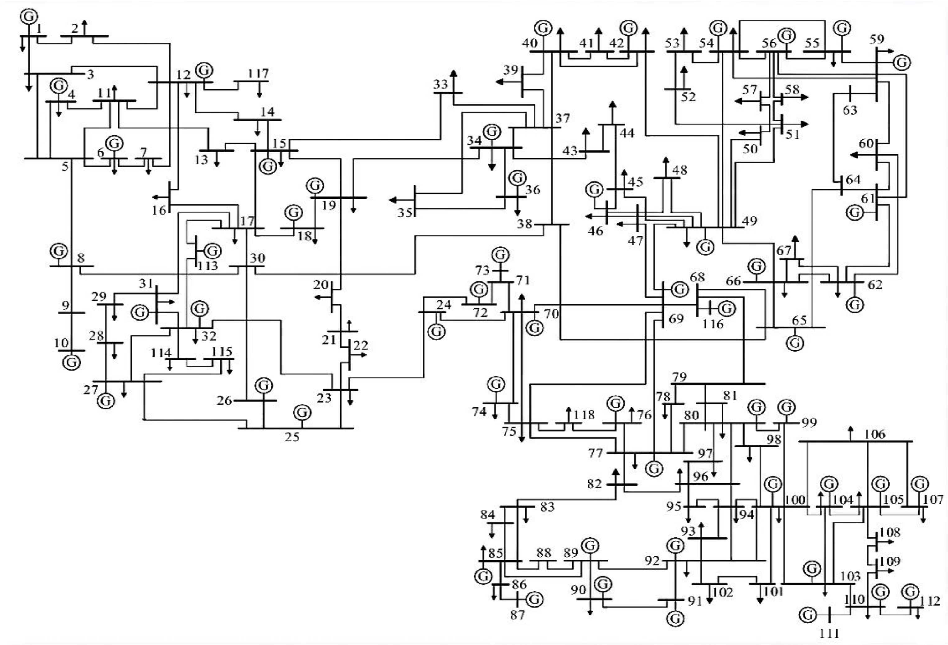
5.1. System Discerption

The proposed model is validated with the modified IEEE 118-node testing system, which is shown in the Figure A1, in Appendix A. The system data are available at [29]. The modified IEEE 118-node system contains ten wind farms, each of which contains 100 double-fed wind turbines (2 MW). The rated power and capacity of the energy storage systems are, respectively, 10 MW and 20 MWh. The costs of upward and downward reserve capacities are set as CNY 20/MW. The locations of the wind farms and energy storage systems are shown in Appendix A. The system voltage limits are set as [0.97, 1.06] p.u. The uncertainty of the system is simulated via Monte Carlo simulation. The corresponding distributions and parameters are set as follows:
(1)
The nodal load power is assumed to follow a normal distribution with a mean value given by the provided standard data and a variance of ±10%. The load correlation coefficient of the connected node is set to 0.15.
(2)
The cut-in, cut-out, and rated wind speeds of wind turbines are, respectively, set as 3 m/s, 25 m/s, and 12 m/s.
(3)
To simulate a fault on branches 18–35, the probability values of fault type and location are adopted from Table 1 and Table 2. The fault recovery time is assumed to follow a normal distribution with a mean value of 350 ms and a standard deviation of 10%.
The non-sequential Monte Carlo sampling method is used to generate 1000 scenarios, and K-MEANS clustering is used to reduce them to 15 typical scenarios.
This paper presents a rolling simulation analysis using the provided case study distribution starting at 10:00 a.m. During the simulation, generation unit 17 (40 MW) experiences a fault at 12:00 p.m. and recovers to the stability condition afterward. At 1:00 p.m., generation units 2, 10, 16, 21, 27, 35, and 43 experience faults. Specifically, the system is in the preventive control stage between 10:00 a.m. and 12:00 p.m. Although a minor fault occurs at 12:00 p.m., the system remains stable after fault recovery, maintaining preventive control. After 2:00 p.m., the system enters the emergency control stage. The time steps in the preventive and emergency control stages are, respectively, 15 min and 0.1 s. The solving times of the two states are 2 h and 8 s. In addition, to further analyze the impacts of the energy storage systems and the reserve requirements of the system, three different system configuration schemes are used for analysis:
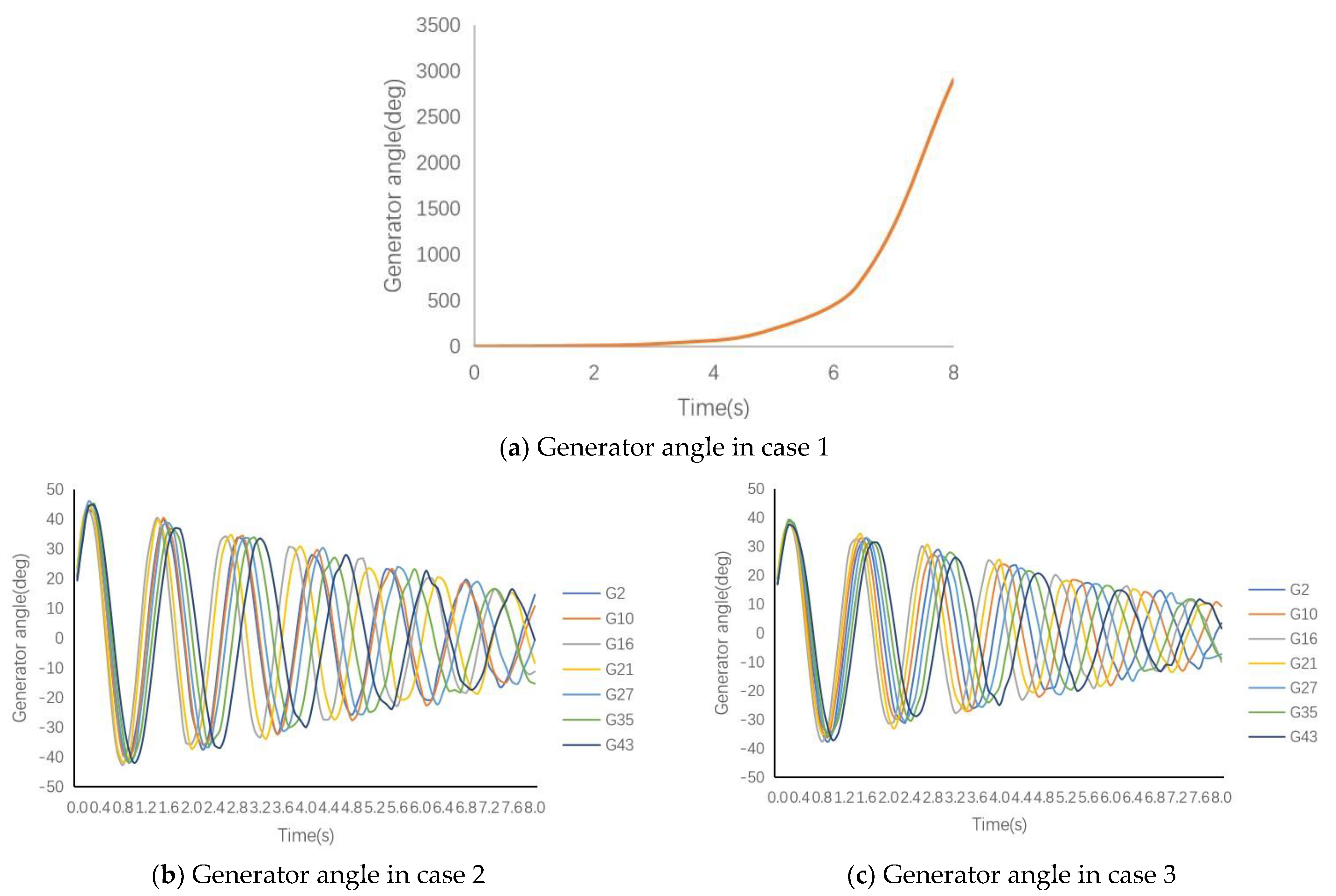
  • Case 1: Reserve and energy storage systems are not considered;
  • Case 2: Only reserve from generation units is considered (energy storage systems are not considered);
  • Case 3: Reserve from both generation units and energy storage systems are considered.

5.2. Optimization Results

5.2.1. Analysis before Failure

From 10:00 a.m. to 11:59 a.m., the system remains fault-free and is in the preventive control stage. In Case 1, the maintenance work of the system remained in the non-optimized state as in the previous moment, and it was still undergoing the preventive control stage. The average cost per hour in this scenario is USD 95,634/h.
In Case 2, although the preventive control stage is initiated, the energy storage participation is not considered, and only the reserve capacity from generation units is considered. Due to the inclusion of the reserve cost of the generation units, the total cost before the fault increases to USD 98,985/h.
In Case 3, the reserve from energy storage systems is considered in the preventive control stage, which causes an increase in the cost before the fault to USD 104,182/h.
In the preventive control stage, the scheduled reserve capacities for Case 2 and Case 3 are illustrated in Figure 3 and Figure 4, respectively.
During the preventive control stage, the system’s demand for the reserve is mainly concentrated on the peak load hours between 11:00 and 12:00. Based on Figure 4 and Figure 5, it can be observed that the scheduled reserve capacities in Case 2 and Case 3 in the preventive control phase can meet the reserve capacity demand during peak load hours. In Case 3, the energy storage systems provide 4.89 MW of upward reserve capacity and 3 MW of downward reserve capacity in the loop. A horizontal comparison reveals that the energy storage systems can provide a certain amount of upward re-serve capacity during peak load hours, fulfilling about 5.4% of the system’s reserve capacity requirement. This would enable other power supply units to remain at high output levels without increasing the operational risk of the system. During valley load hours, the energy storage system can provide a certain amount of downward reserve capacity to ensure the optimal utilization of resources.
The probabilities of the system stability with the three cases are shown in Figure 5.
In this scenario, the other probability indicators of the system do not meet the requirements; for instance, in the case of a three-phase short circuit fault with a fault lo-cation near node 22, ① the probability of node 21 voltage magnitude being in the range of [0.97, 1.06] is only 0.2, which is lower than the required probability of 0.95; ② the probability of the transmission line flows being within the limit is only 0.6; and ③ the probability of the system attaining transient stability is 0.54. Additionally, there are differences in safety margins among the three schemes. In Case 1, for probability indicators, such as the probability of node voltage magnitude, the probability of the trans-mission line flows being within the limit and the probability of then attaining transient stability are both below the threshold. As a result, the obtained safety margin is only 0.52. In Case 2 and Case 3, the probability indicators of the system are improved to a certain extent, and their stability margins reach 0.95 and 1.00, respectively. Particularly in Case 3, by optimally controlling the reserve capacity and considering energy storage systems’ participation, the system is better secured.

5.2.2. Analysis on Single Failure

At 1:00 p.m., generation unit 17 (40 MW) encounters a fault. The power angle trajectories of the generation unit in all three cases are shown in Figure 6.
In Case 1 and Case 2, the system loses stability in 2–4 s after the fault occurs. Case 1 loses stability first due to the lack of reserve support. In contrast, the re-serve capacity of Case 3 was adequate to make up for the gap caused by the fault. The power angle oscillated within 50 degrees, and the power angle deviation gradually de-creases over time. The system shows a tendency towards stability recovery.

5.2.3. Analysis on Multiple Faults

At 2:00 p.m., generation units 2, 10, 16, 21, 27, 35, and 43 experience faults. With-out implementing emergency control measures, the rotor angle trajectories of the generation units in all three cases are shown in Figure 7.
As shown in Figure 7, in all three cases, the system becomes unstable after the faults occur in the absence of emergency control measures. Like the single fault case, the system in Case 1 becomes unstable first; by contrast, the system in Case 3 can re-main stable for some time, relying on the reserve from the generation units and the energy storage systems, but it will eventually become unstable. The rotor angle trajectories for generation units subjected to emergency control measures are shown in Figure 8.
The system in Case 1 will still become unstable after 4 s of emergency control as it does not account for the reserve capacity from generation units and energy storage systems, which results in significant power shortages during multiple faults. In such a case, the system cannot compensate for the power shortage; hence, it loses stability. By contrast, Case 2 considers the reserve capacity from generation units, which helps reduce the deviation of the generator power angle within 8 s after the emergency control, indicating a trend towards stable operation. In comparison, for Case 3, which further considers the reserve from energy storage system, the deviation of the generator power angle is reduced by approximately 10%, and it exhibits a quicker recovery to stable operation. In Appendix A, Figure A2 and Figure A3 illustrate the reserve adjustment schemes.
The costs of the three cases in the emergency control stage are shown in Table 3.
Among the three cases, Case 1 incurs the highest cost since it fails to account for the reserve capacity of generation units and the energy storage system, resulting in difficulty stabilizing the system. In contrast, Case 2 considers the cost of reserve during the preventive control stage, and the inclusion of reserve from generation units helps the system to remain stable, which reduces the cost by 5.1% compared to that of Case 1. Moreover, Case 3 further considers the reserve capacity from energy storage systems and has the lowest adjustment cost; it reduces the cost by 9.6% compared to Case 1 and by 2.2% compared to Case 2.

5.2.4. Algorithm Comparison

To demonstrate the effectiveness of the proposed improvement to the solving algorithm, Case 3 is taken as an example. The improved MOPSO (IMOPSO) and the traditional MOPSO algorithms are used to solve the optimization problem for each objective. The results are compared in Table 4.
Table 4 reveals that the comprehensive cost obtained by the IMOPSO algorithm is 8.63% lower than that obtained by the traditional MOPSO, while the iteration speed of IMOPSO is 20.76% fast than that of the traditional MOPSO, demonstrating the effectiveness of the algorithm improvement proposed in this paper, which enhances the global search capability of the algorithm.

6. Conclusions

This paper proposes a two-stage preventive control optimization model that ad-dresses the possible system transition instability issue caused by the uncertainties introduced by different system components considering the balance of economy and system safe operation. The first stage of the model is used to obtain an optimal operation schedule which guarantees a high probability of the system being stable and a low operation cost. The second stage is applied to respond to the emergency after the occurrence of any faults that may result a stability issue. Furthermore, the multi-objective particle swarm optimization algorithm based on entropy-TOPSIS is adopted to accelerate the solving process of the two-stage model. The case study shows that with the proposed model, while pursuing economics, the safety and stability mar-gin of the system can be reduced. In addition, when multiple faults occur and threaten the system’s stability, emergency control can help the system meet the satisfy the stability margin requirements with a slightly higher cost on the top of the schedule obtained in the preventive control stage.

Author Contributions

Q.N.: conceptualization, methodology, validation, project administration. J.S.: Methodology, software, writing—original draft editing. X.Z.: software, validation, writing—original draft. T.Z.: methodology, validation. Z.S. and M.Z.: software, formal analysis. All authors have read and agreed to the published version of the manuscript.

Funding

This research was funded by the State Grid Zhejiang Electric Power Co., Ltd. Technology Project (5211WZ220005).

Conflicts of Interest

The authors declare no conflict of interest.

Appendix A

Figure A1. IEEE 118-node system.
Processes 11 02258 g0a1
The ten wind farms are located at nodes 7, 14, 22, 44, 63, 60, 79, 80, 83, and 101. The energy storage systems are located at nodes 31, 52, 81, and 106.
Figure A2. Reserve from generation units in Case 2.
Processes 11 02258 g0a2
Figure A3. Reserve from generation units in Case 3.
Processes 11 02258 g0a3

References

  1. Chen, G.; Dong, Y.; Liang, Z. Analysis and reflection on high-quality development of new energy with Chinese characteristics in energy transition. Proc. CSEE 2020, 40, 5493–5506. [Google Scholar]
  2. Zhang, N.; Hu, Z.; Han, X.; Zhang, J.; Zhou, Y. A fuzzy chance-constrained program for unit commitment problem considering demand response, electric vehicle and wind power. Int. J. Electr. Power Energy Syst. 2015, 65, 201–209. [Google Scholar] [CrossRef]
  3. Wong, W.C.; Chung, C.Y.; Chan, K.W.; Chen, H. Quasi-Monte Carlo based probabilistic small signal stability analysis for power systems with plug-in electric vehicle and wind power integration. IEEE Trans. Power Syst. 2013, 28, 3335–3343. [Google Scholar] [CrossRef]
  4. Hasan, K.N.; Preece, R.; Milanović, J.V. Existing approaches and trends in uncertainty modelling and probabilistic stability analysis of power systems with renewable generation. Renew. Sustain. Energy Rev. 2018, 101, 168–180. [Google Scholar] [CrossRef]
  5. Indhumathy, D.; Narmatha, D.; Meenambika, K. Mixture Weibull probabilistic model in Wind Turbine Power Analysis. J. Phys. Conf. Ser. 2021, 1916, 012109. [Google Scholar] [CrossRef]
  6. Alrashidi, M. Estimation of Weibull Distribution Parameters for Wind Speed Characteristics Using Neural Network Algorithm. Comput. Mater. Contin. 2023, 75, 1073–1088. [Google Scholar] [CrossRef]
  7. Xie, G.-L.; Zhang, B.-H.; Li, Y.; Mao, C.-X. Harmonic propagation and interaction evaluation between small-scale wind farms and nonlinear loads. Energies 2013, 6, 3297–3322. [Google Scholar] [CrossRef] [Green Version]
  8. Faried, S.; Billinton, R.; Aboreshaid, S. Probabilistic evaluation of transient stability of a power system incorporating wind farms. IET Renew. Power Gener. 2010, 4, 299–307. [Google Scholar] [CrossRef]
  9. Fang, D.; Jing, L.; Chung, T. Corrected transient energy function-based strategy for stability probability assessment of power systems. IET Gener. Transm. Distrib. 2008, 2, 424–432. [Google Scholar] [CrossRef]
  10. Mele, F.M.; Zarate-Minano, R.; Milano, F. Modeling Load Stochastic Jumps for Power Systems Dynamic Analysis. IEEE Trans. Power Syst. 2019, 34, 5087–5090. [Google Scholar] [CrossRef]
  11. Ye, S.; Xiaoru, W.; Shu, Z. Power system probabilistic transient stability assessment based on Markov Chain Monte Carlo method. Trans. China Electrotech. Soc. 2012, 27, 168–174. [Google Scholar]
  12. Saraninezhad, M.; Ramezani, M.; Falaghi, H. Probabilistic Assessment of Wind Turbine Impact on Distribution Networks by Using Latin Hypercube Sampling Method. In Proceedings of the 2022 9th Iranian Conference on Renewable Energy & Distributed Generation (ICREDG), Mashhad, Iran, 23–24 February 2022; IEEE: Piscataway, NJ, USA, 2022. [Google Scholar] [CrossRef]
  13. Yan, Y.; Sun, N.; Zhang, N. Evaluation of unavailability risk of the security and stability control system of power systems based on optimization of the preventive maintenance period. Power Syst. Prot. Control. 2021, 49, 139–146. [Google Scholar]
  14. Peng, Y.; Dong, X.; Zhou, H. Reliability evaluation of power grid security and stability control system. Power Syst. Prot. Control. 2020, 48, 123–131. [Google Scholar]
  15. Li, X.; Zhou, S.; Xu, X.; Lin, L.; Wang, D. The Reliability Analysis Based on Subsystems of $(n, k) $-Star Graph. IEEE Trans. Reliab. 2016, 65, 1700–1709. [Google Scholar] [CrossRef]
  16. Etemadi, A.H.; Fotuhi-Firuzabad, M. Design and routine test optimization of modern protection systems with reliability and economic constraints. IEEE Trans. Power Deliv. 2011, 27, 271–278. [Google Scholar] [CrossRef]
  17. Wang, Q.; Martinez-Anido, C.B.; Wu, H.; Florita, A.R.; Hodge, B.-M. Quantifying the economic and grid reliability impacts of improved wind power forecasting. IEEE Trans. Sustain. Energy 2016, 7, 1525–1537. [Google Scholar] [CrossRef]
  18. Bao, Y.; Zhang, J.; Yi, L.; Xu, T.; Ren, X.; Wu, F. Prevention and Control Method of Security and Stability Risk for Power System with Large-scale Wind Power Integration. Autom. Electr. Power Syst. 2022, 46, 187–194. [Google Scholar]
  19. Parvin, M.; Yousefi, H.; Noorollahi, Y. Techno-economic optimization of a renewable micro grid using multi-objective particle swarm optimization algorithm. Energy Convers. Manag. 2023, 277, 116639. [Google Scholar] [CrossRef]
  20. Babypriya, B.; Renoald, A.J.; Shyamalagowri, M.; Kannan, R. An experimental simulation testing of single-diode PV integrated mppt grid-tied optimized control using grey wolf algorithm. J. Intell. Fuzzy Syst. 2022, 43, 5877–5896. [Google Scholar] [CrossRef]
  21. Zao, T.; Jia, L.; Pingliang, Z. A multi-timescale operation model for hybrid energy storage system in electricity markets. Int. J. Electr. Power Energy Syst. 2022, 138, 107907. [Google Scholar] [CrossRef]
  22. Ni, Y.; Chen, S.; Zhang, B. Theory and Analysis of Dynamic Power System; Tsinghua University Press: Beijing, China, 2022. [Google Scholar]
  23. Shi, H.B.; Chen, G.; Ding, L.J.; Han, X.; Zhang, Y.; Chen, Z. PID parameter optimization of hydro turbine governor considering the primary frequency regulation per-formance and ultra-low frequency oscillation suppression. Power Syst. Technol. 2019, 43, 221–226. [Google Scholar]
  24. IEEE Std 421.5-2016; IEEE Recommended Practice for Excitation System Models for Power System Stability Studies. IEEE: Piscataway, NJ, USA, 2016; pp. 1–207, Revision of IEEE Std 421.5-2005.
  25. Parida, A.; Paul, M. A Novel Modeling of DFIG Appropriate for Wind-Energy Generation Systems Analysis. In Proceedings of the 2022 IEEE 10th Power India International Conference (PIICON), New Delhi, India, 25–27 November 2022; pp. 1–6. [Google Scholar]
  26. Li, W.; Yao, X.; Zhang, T.; Wang, R.; Wang, L. Hierarchy Ranking Method for Multimodal Multiobjective Optimization with Local Pareto Fronts. IEEE Trans. Evol. Comput. 2022, 27, 98–110. [Google Scholar] [CrossRef]
  27. Parvin, J.R.; Vasanthanayaki, C. Particle swarm optimization-based energy efficient target tracking in wireless sensor network. Measurement 2019, 147, 106882. [Google Scholar] [CrossRef]
  28. Campos, M.; Krohling, R.A. Entropy-based bare bones particle swarm for dynamic constrained optimization. Knowledge-Based Syst. 2016, 97, 203–223. [Google Scholar] [CrossRef]
  29. Shahidehpour, M.; Yamin, H.; Li, Z. Market Operations in Electric Power Systems: Forecasting, Scheduling, and Risk Management; Wiley: New York, NY, USA, 2002. [Google Scholar]
Figure 1. The Pareto front value.
Processes 11 02258 g001
Figure 2. Flowchart of the solving process of the preventive control model.
Processes 11 02258 g002
Figure 3. The scheduled reserve capacities in Case 2.
Processes 11 02258 g003
Figure 4. The scheduled reserve capacities in Case 3.
Processes 11 02258 g004
Figure 5. The probabilities of the system stability with the three cases.
Processes 11 02258 g005
Figure 6. Power angle trajectories of the generation unit.
Processes 11 02258 g006
Figure 7. Rotor angle trajectory of generators at 2:00 p.m.
Processes 11 02258 g007
Figure 8. Rotor angle trajectory of generation units at 2:00 p.m. with emergency control.
Processes 11 02258 g008
Table 1. Probabilities of different fault types.
Fault TypeThree-Phase Two-Phase Single-Phase Phase-to-Phase Total
Statistical results %12934100
Table 2. Costs of preventive control stage.
CasesCase 1Case 2Case 3
Costs (USD/h)95,63498,985104,182
Table 3. Costs of the emergency control stage of the three cases.
CasesCase 1Case 2Case 3
Costs ($/h)98,42192,11290,101
Table 4. Results of different optimization algorithms.
AlgorithmCosts ($)IterationsAverage Calculation Time for Each Iteration
MOPSO98,6131834.52 s
IMOPSO90,1011454.43 s
Disclaimer/Publisher’s Note: The statements, opinions and data contained in all publications are solely those of the individual author(s) and contributor(s) and not of MDPI and/or the editor(s). MDPI and/or the editor(s) disclaim responsibility for any injury to people or property resulting from any ideas, methods, instructions or products referred to in the content.

