In Situ Indoor Air Volatile Organic Compounds Assessment in a Car Factory Painting Line

Abstract

Proper working conditions must be one of the employers’ main concerns in any type of company but particularly in work locations where the employees are chronically exposed to hazardous compounds, like factories and production lines. Regarding this challenge, the present research addresses the mapping of a car factory painting line to possibly toxic volatile organic compounds emitted by all the coatings and chemicals used during the work shifts for the future evaluation of employees’ exposure. For the first time, a Gas Chromatography–Ion Mobility Spectrometry device was employed for the in situ detection of volatile organic compounds in an automotive factory. A total of 26 analytes were detected at nine different locations, of which 15 VOCs were accurately identified. Pure chemical-grade substances were used for the development of the VOC database. Although quantitative analysis was not the goal of this study, a calibration model was presented to one analyte for exemplificative purposes. Relative intensity profiles were plotted for all locations, revealing that some indoor VOCs can reach intensity levels up to 60 times higher than in outdoor air samples. The achieved results proved that the painting line has an abundant number of VOCs emitted from different sources and may lead to serious health risks for the employees. Additional studies shall be developed in the painting line for quantitative evaluation of the existing VOCs and their influence on the employees’ health conditions.

1. Introduction

Employees’ health preservation and good working conditions must be among the most supervised and regulated issues in any type of company. Factories and production lines, where exposure to dangerous and toxic compounds is an everyday occurrence, should have strict legislation and precise systems for continuously monitoring and controlling the conditions to which the employees and workers are subjected.

This work intends to describe and assess a complex and serious scenario, the exposure of the workers of a car factory painting line to the volatile organic compounds (VOCs) emitted by the chemicals utilized during the coating processes and, in parallel, to evaluate for the first time, the suitability of a specific analytical technique, gas chromatography–ion mobility spectrometry (GC-IMS), for the detection, identification, and quantification of those VOCs in such a potentially hazardous environment.

1.1. Volatile Organic Compounds

Volatile organic compounds merge two very relevant attributes. The covalent bonding between carbon atoms and several functional groups, like alcohol, ketones, or ether, characterizes their organic nature [1,2,3,4]. In addition, VOCs are volatile at room temperature since they present a vapor pressure of at least 10 Pa at 293.15 K (20 °C) [5].

The VOCs are directly related to a vast number of daily activities and can be released by an immense amount of commonly used objects. Furniture, clothes, and building materials are among the main sources of VOCs in residential areas. Daily activities like cooking, smoking, or cleaning, and the products related to these activities, like cleaning detergents, personal care products, creams, perfumes, tobacco, or food, are equally abundant sources of this type of analytes [6,7,8,9,10,11,12]. In an industrial context, VOCs are emitted by a very diverse range of sources, namely, paints, varnishes, waxes, solvents, plastics, rubbers, and many other chemical-based products [13,14].

Due to being volatile at room temperature, VOCs can be present, traverse, or even be emitted by several biological structures. The pulmonary (respiration), ocular (lacrimal fluid), and cutaneous (perspiration) tissues are, in fact, the most well-known ways of VOC exchange between the exterior and the interior of the human organism. The presence of VOCs in the body can lead to the processing of inflammation and cause mutations by oxidative stress in the human cells, so they are directly responsible for a vast range of health conditions and pathologies [15]. Eyes allergies and skin irritation are common reactions to the presence of VOCs. Methyl ethyl ketone, also known as 2-butanone, for example, has been studied as a cause of skin and eye irritation, in scenarios of short-term exposure, and for neurological, liver, and kidney effects, in cases of chronic exposure [16]. Considering the threshold limit value (TLV) index, an index defined by the United States National Institute for Occupational Safety and Health (NIOSH) to characterize the maximum concentration level to which an employee can be repeatedly exposed throughout his/her professional life without experiencing any relevant health impacts, 2-butanone represents a direct risk for life if a person is exposed to 200 ppm_v or more [17]. Asthma, chronic obstructive pulmonary disease, and other inflammatory pathologies of the respiratory tract are also among the most frequent effects of prolonged exposure to VOCs [18,19,20,21,22]. Lung, breast, and some other severe forms of cancer have recently been related to exposure to hazardous VOCs. In fact, benzene (TLV: 10 ppm_v), trichloroethylene (TLV: 50 ppm_v), chloroform (TLV: 10 ppm_v), and formaldehyde (TLV: 0.3 ppm_v), all common and very well-known VOCs, have been recently identified as carcinogenic compounds [17,23,24,25,26,27].

As mentioned, the sources of VOCs are vast and diverse in both indoor and outdoor environments. They are present in all kinds of locations, from recreation to working sites, and from private to public utilities. A car factory painting line is no exception [13,14]. The process of painting a car body is intricate and involves numerous phases; however, all of them require the use of products that are potential VOC-emitting sources [28,29]. In fact, a scientific study estimated that the total emission of VOCs by a car factory ranges from 1.18 to 4.30 kg per produced vehicle, an enormous and very dangerous quantity [30].

In the first step, the car chassis is immersed in two chemical baths. To do so, giant wells filled with chemical solutions are used. The phosphating bath consists of a solution of phosphoric acid saturated with metallic phosphate whose purpose is to protect the metal against corrosion and increase adherence to the coatings. The cataphoresis bath, in its turn, covers the entire metal surface with a thin electrically charged epoxy layer that enables a uniform application of the coatings throughout the car body. Once dried in industrial-size ovens, the chassis is transported to the next section. Here, the primer and the ink are applied to the surface by robotic arms. These automatized processes involve the formation of coating clouds that are projected into the metal surface previously treated during the chemical baths. Then, high-pressure jets are used for projecting the varnish into the already-colored chassis. Right after it, a group of employees uses several tools (rotatory devices and tissues) to manually polish the surface with wax. Finally, each chassis is visually inspected by the line workers, to find eventual imperfections or inconsistencies in the painting [13,28,29,31]. Figure 1 schematizes the described steps of the car factory painting line.

As mentioned, many chemical compounds are employed during the entire painting process meaning that the indoor air is predictably filled with a vast number of VOCs whose consequences for the employees must be addressed. Although the employees of the car factory use protective gear, like activated charcoal masks, glasses, and jumpsuits, they are not completely protected from the huge variety of VOCs existing in the interior of the painting line, especially if we consider the number of hours (at least eight hours) of daily exposure to such a hazardous environment. Due to all these facts, the identification and quantification of volatile organic compounds is a mandatory task. In this work, the very first steps are given to completely assess all the characteristics of the indoor air of the painting line and prospectively evaluate the impacts and consequences on the employees’ health [32].

1.2. Gas Chromatography–Ion Mobility Spectrometry

There are several analytical techniques, specifically spectroscopic, spectrometric, and chromatographic techniques, which enable the analysis of samples of VOCs [33,34,35]. This work intends to evaluate, for the first time, Ion Mobility Spectrometry coupled with Gas Chromatography as an in situ, suitable, reliable, precise, and accurate technique for the detection, identification, and quantification of all the VOCs existing on the painting line [36].

Ion mobility spectrometry has gained relevance, over the past two decades, as one of the most promising analytical techniques in several distinct scientific fields, namely, air quality control, health assessment, security purposes, food quality assessment, and many others [37,38]. The coupling, in a single device, of both Gas Chromatography (GC) and Ion Mobility Spectrometry (IMS), creates an enhanced analytical technique, GC-IMS, with extraordinary selectivity and sensitivity, analytical flexibility and simplicity, rapid monitoring capability, very good detection limits (ppb_v–ppt_v), and good precision [36,39,40]. Concisely, GC-IMS can be used for in situ detection, identification, and differentiation of volatile organic compounds based on their intrinsic characteristics, like size, weight, or shape, without requiring any additional chemical or any previous and complex sample preparation [36].

Once introduced into the device, the sample undergoes a pre-separation process where the analytes are differentiated by their capability of adsorbing to the chromatographic column. Each analyte of the sample requires a specific time to elute from the column, known as retention time, $r_t$ [39]. Then, the pre-separated compounds enter the IMS ionization chamber where they are ionized by an ionization source. Among the possible sources, tritium (³H), nickel (⁶³Ni), and X-rays are the most common [41,42]. The spontaneous emission of a ${\beta }^{-}$ particle instigates a reaction with an inert gas present inside the spectrometer, typically nitrogen ($N_2$). This reaction leads to the formation of background ions of hydrogen ($N_2^{+}$) [36,43]. In their turn, the background ions, also known as primary ions, react with the molecules of $H_{2}O$ (they can also react with $N{H}_3$ and $NO$ molecules) present inside the IMS tube, forming new ions, named reactant ions. Finally, these new ions (${\left(H_{2}O\right)}_n{H}^{+}$, ${\left(H_{2}O\right)}_{n}N{H}_4^{+}$, or ${\left(H_{2}O\right)}_{n}N{O}^{+}$) constitute the reactant ion peak (RIP) and they react with the sample analytes [34,36,43,44]. As an example, if the compound M is an arbitrary analyte present in the original sample, its reaction with the reactant ions occurs as follows:

$$M+{\left(H_{2}O\right)}_n{H}^{+}\leftrightarrow M{\left(H_{2}O\right)}_{n-x}{H}^{+}+x{H}_{2}O,$$

(1)

The ions formed in this reaction, called product ions, are a connection between a proton and a molecule, so they correspond to protonated monomers of the compound M. In scenarios where the concentration of M is higher, the product ions can suffer a second reaction with the remaining M molecules. This reaction leads to the formation of protonated dimers of compound M, as represented in Equation (2) [45,46,47]. Even though they are not so common, larger clusters can also be formed.

$$M+M{\left(H_{2}O\right)}_{n-x}{H}^{+}\leftrightarrow M_2{\left(H_{2}O\right)}_{n-\left(x+i\right)}{H}^{+}+i{H}_{2}O,$$

(2)

Once created, all product ions are exposed to a weak and homogeneous electric field that accelerates them across the IMS tube. During this process, the ions suffer collisions with the molecules of the drift gas present inside the tube. The continuous acceleration-collision process makes the velocity of the ions tend to a constant value, denominated by drift velocity, $v_d$. When the ions finally reach the end of the IMS tube, they are detected by a Faraday plate, which registers the time required by each ion to traverse the drift tube and its intensity [36,43,44,48].

The drift velocity is a specific value for each compound and its correlation with the electric field, E, is given by the ion mobility constant, K, as represented in Equation (3):

$$K=\frac{v_d}{E},$$

(3)

As with any velocity, drift velocity can also be represented by the quotient between the traversed distance, L, and the time. This temporal value corresponds to the time each analyte takes to cross the ion mobility spectrometer tube, and it is defined as drift time, $d_t$ [49,50]. In this way, Equation (3) can be written in a new format:

$$K=\frac{L}{E·t_d},$$

(4)

Since the ion mobility constant depends on temperature and pressure conditions, it is common to normalize it to standard environmental values of temperature (T₀ = 273.15 Kelvin) and pressure (P₀ = 760 Torr) [34,36,51]. The normalized ion mobility constant, K₀, can be written as:

$$K_0=K\left(\frac{P}{P_0}\right)\left(\frac{T_0}{T}\right),$$

(5)

A schematic of the described steps of a complete GC-IMS analysis can be found elsewhere [47].

A three-dimensional spectrum containing all the detected VOCs is plotted at the end of each analysis. This spectrum represents both the retention (s) and the drift (ms) times of all the analytes present in the initial sample, as well as their intensities (V). Figure 2 exemplifies an IMS spectrum represented in two- and three-dimensional views, respectively. The long red column across the spectrum corresponds to the aforementioned reactant ion peak (RIP). As addressed, each volatile compound has its specific drift (x-axis) and retention (y-axis) times; in this way, all the individual peaks seen in the spectrum are a particular VOC from the analyzed sample. Regarding the intensity (z-axis), a color scheme is used to illustrate its different levels among different peaks.

Both the drift and retention times, as well as the ion mobility constant, are compound-specific values, in this way, they enable the correct and accurate identification of all the VOCs existing in the analyzed sample. The intensity, in its turn, can be directly related to the concentration of each analyte. Together, the three coordinates of the spectrum enable the qualification and quantification of a sample by IMS [49,52]. Nonetheless, the challenges of calibrating a GC-IMS device to be able to convert the detected intensities into concentration values and, consequently, quantify the identified analytes are well known and well addressed in the literature [53,54].

2. Materials and Methods

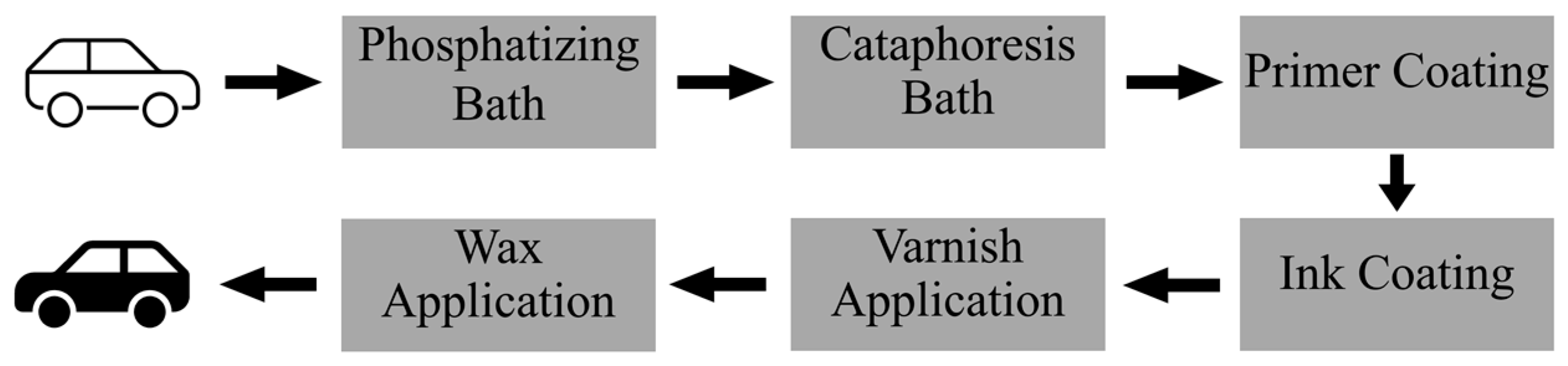
2.1. Analyzed Locations

Based on their characteristics, a total of nine locations of the painting line were considered for this work (one outdoor and eight indoor locations): i—phosphatizing bath, ii—cataphoresis bath, iii—primer application, iv—ink application, v—varnish application, vi—wax application, vii—ceiling of the factory, viii—office of the painting line head, and ix—outdoor air (reference air).

Even without access to the exact composition of the bath solutions, the large amount and diversity of chemicals used in both phosphatizing (i) and cataphoresis (ii) baths make these locations considerably interesting for air analyses. The primer (iii), ink (iv), varnish (v), and wax (vi) coatings, in their turn, are applied to the chassis by automatized robotic arms; however, the presence of employees inside these locations is extremely common. In this way, due to this continuous exposure, all these four locations were also considered of special interest for air analyses. The extractors and air purification systems are assembled in the factory ceiling (vii), so it is important to assess the presence of VOCs near these systems. The air from the office of the painting line manager was also analyzed due to being a room isolated from the painting line but, usually, very crowded. Finally, since they are free of interference from the painting line emissions, samples of the outdoor air were collected and analyzed to act as reference air.

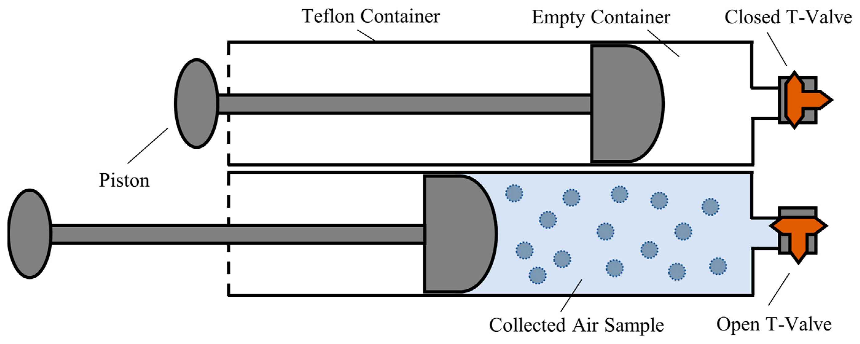
2.2. Air Collection Methodology

To not expose the device to possibly damaging or destructive scenarios, in the interior of the painting line, and to not disrupt the normal working routines of the employees, the spectrometer was assembled in an office located in a central position near all the locations under analysis. The air samples were collected from nine different locations with a chemically inert Teflon container (1 L volume) with an accoupled T-valve and transported to the spectrometer. To do so, the T-valve was opened and the piston of the Teflon container was manually pulled until the container was filled with air from the target location. Then, the T-valve was closed to prevent additional exchanges between the sample and exogenous contaminants, and the container was transported to the room of the GC-IMS device. The transfer time of the samples was always inferior to three minutes, a procedure that ensured the preservation of the original specificities of the sample by avoiding temperature and humidity variations and, as mentioned, interactions with exogenous compounds. The repeatability of the data and, consequently, the suitability of this collection procedure were assessed and are addressed below. Figure 3 schematizes the process of collecting the air samples.

2.3. Gas Chromatography–Ion Mobility Spectrometry

In this study, a tandem equipment GC-IMS manufactured by G. A. S. (Dortmund, Germany) was used. The apparatus was equipped with a 300 MBq ionization source of tritium (H3-β radiation) and a 98 mm length drift tube with a 5 kV switchable polarity. The electric field intensity employed in the drift tube was 500 V/cm. The chromatographic column assembled in the device was an MXT-200 model with 30 m of length and 0.53 mm of internal diameter coated with stainless steel with a mid-polar stationary phase of trifluoropropylmethyl polysiloxane with a thickness of 1 μm. The complete list of experimental protocol parameters of the GC-IMS device used for the analyses is summarized in

Table 1. Parameters and features of the GC-IMS device.

Parameters	Values	Units
Sample Loop Volume	1	mL
GC Column Model	MXT-200	-
GC Column Length	30	m
GC Column Diameter	0.53	mm
GC Temperature	343.15	K
Gas Nature	Purified Air	-
Carrier Gas Flow	10	mL/min
Drift Gas Flow	150	mL/min
Ionization Source	Tritium-β Radiation	-
Ionization Intensity	300	MBq
Ionization Polarity	Positive	-
Drift Region Length	9.8	cm
Drift Potential Difference	5	kV
IMS Temperature Range	297.15–301.15	K
IMS Pressure Range	757–760	Torr
Electrical Field Intensity	500	V/cm
Resolving Power Range	65–70	-
Analysis Duration	300	s

.

The CG-IMS equipment was connected to the Circular Gas Flow Unite (CGFU) from G.A.S., Dortmund, which supplies purified air as a carrier gas. The use of a CGFU offers portability to the equipment, which is of particular interest for the present study due to the possibility of using this analytical instrument outside of the laboratory for in situ measurements.

2.4. Assessment of VOCs

Ten consecutive air samples were collected from each location and analyzed by GC-IMS within a 15 min interval. For each measurement, a three-dimensional spectrum was created and saved. All the obtained spectra were processed with the LAV software (version 2.2.1.—G. A. S. Dortmund). The values of intensity, drift time, and retention time of each compound were exported and statistically processed for the assessment of the VOCs found in all samples.

As mentioned before, both the drift and retention times and the ion mobility constant are compound-specific values; i.e., they can be used to accurately distinguish between any analyte, even between structurally similar compounds. Thus, the VOCs detected in the air samples were identified by comparing both these parameters with the corresponding values registered in a pre-developed database. To develop this library of analytes, pure samples (20 μL) of VOCs were prepared in 20 mL glass vials. Once the thermodynamic balance between the liquid and the gaseous parts in the interior of the vial was reached, 2 mL of headspace was collected with a syringe and a needle and inserted into the spectrometer. A schematic representation of the used methodology can be consulted elsewhere [37]. Once analyzed, their specific drift and retention times were registered in the database. In addition, the normalized ion mobility constant of each analyte was calculated, as described in Equations (3)–(5), and included in the database. This library of compounds is an underdevelopment database whose content is often increased. At the time of this work, the database consisted of 269 volatile organic compounds prepared and analyzed with the described methodology.

For classification purposes, the drift and retention times of the analytes detected in the samples of indoor air were, then, crosschecked with the values registered during the database development, leading to their rapid and precise identification.

Regarding the intensity, the third value of the three-dimensional spectrum was used to plot a profile of relative intensity level for the VOCs existent in each one of the analyzed locations. Such profiles enabled a direct comparison between the air composition of the distinct sites, and a perception of the concentration levels of each analyte in the original sample.

Initially, the average value of the intensities was calculated for all the detected peaks and each location. Then, the relative intensity was determined by the ratio between each average intensity and the respective intensity value in the outdoor samples; i.e., the intensity values of each VOC in the indoor air samples were normalized in relation to the intensity levels of each VOC in the outdoor air. This is equivalent to stating that the intensity of each compound in the outdoor air samples is taken as the zero value of the graphs plotted for the indoor locations. As a result, if a compound exhibits intensity values above zero, this means that the intensities are higher in the studied location than they are in outdoor samples. On the other hand, if a compound intensity value is under the zero axis, this means that its intensity is lower in the location than it is in the air samples from the outside environment. To simplify the representation of the results, the relative intensities of the monomer, dimer, and trimer of a specific analyte were added, and the profiles were represented in individual graphs. Further details about the used procedure are given in due time.

Finally, aiming to assess the level of concentrations existent in the analyzed air samples, a calibration procedure was developed and applied to our data. As mentioned, the process of calibrating the relationship between the intensity detected during the GC-IMS analysis and the corresponding concentration is a rather complex methodology; nonetheless, it was possible to assess the concentration levels for one of the detected analytes, as exposed in due time.

Further details regarding the used procedure can be consulted elsewhere [54]; however, it is relevant to mention that the methodology for calibrating the concentration of the analytes was based on the emissions of permeation tubes containing the target analyte. These tubes were kept in the interior of a thermogravimetric chamber whose main purpose was to control the emissions of the tube considering its mass loss ratio over time. A constant flow of purified air was used to carry the emissions from the chamber into the GC-IMS. As addressed in the literature, a logarithmic regression was adjusted to the obtained data, leading to a mathematical model that enabled the calculation of the original concentrations existent in the samples considering the intensity levels detected by the spectrometer [52,54].

3. Results and Discussion

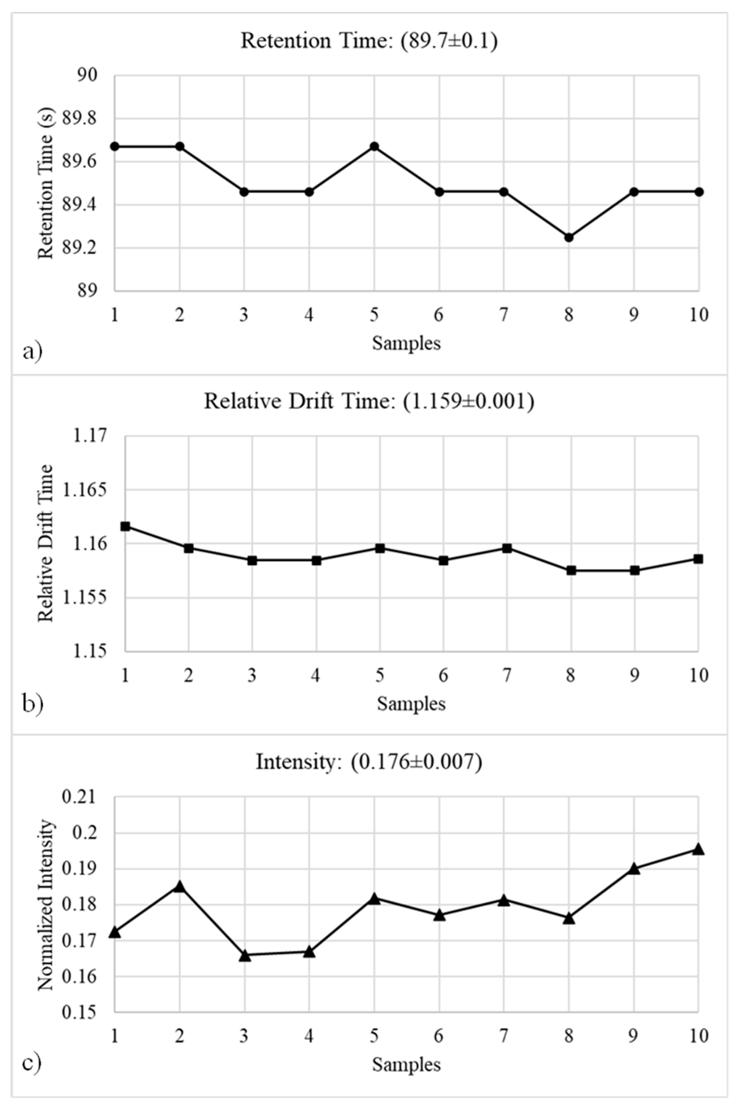
3.1. Data Repeatability

A total of 90 spectra were obtained from all the measurements performed at the nine locations. The quality control of the method was assured by the consecutive measurements of the ten replicates from each location as well as by the measurements of the blank spectra before each experimental run of samples. Aiming to assess the precision and analytical performance of the method, the repeatability for each value of GC-IMS spectra (retention time, relative drift time, and intensity) for every analyte was statistically analyzed. The overall precision is up to 1.2% for the retention time, 0.1% for the relative drift time, and 4.1% for the normalized intensity. For representation purposes, Figure 4 illustrates the variability graphs for a randomly selected analyte (dimer of acetone) analyzed in a location randomly selected (phosphatizing bath). It is important to state that the mean values for the ten replicates (n = 10) and respective standard deviation of the retention time, relative drift time, and normalized intensity for these representative analytes were (89.7 ± 0.1), (1.159 ± 0.001), and (0.176 ± 0.007), respectively. Similar repeatability results were achieved for all the remaining analytes detected in all nine locations.

It is worth saying that all ten consecutive sample measurements from each location were always collected and transported with the mentioned Teflon pump. Since these conditions were accurately kept, one can state that the collection procedure is suitable for the preservation and transportation of the air samples; otherwise, the standard deviation for the average values of normalized intensity would be considerably higher and, consequently, the data would have no statistical validity nor would be repeatable.

From the achieved data analysis, it is possible to state that the proposed method demonstrates a good performance for in situ VOC analysis by GC-IMS showing a full capability of ensuring the repeatability and, consequently, the statistical validity of the collected data. Furthermore, the small standard deviation achieved between 10 consecutive measurements reinforces a good method precision and the suitability of this technology for the analysis of air samples in industrial scenarios.

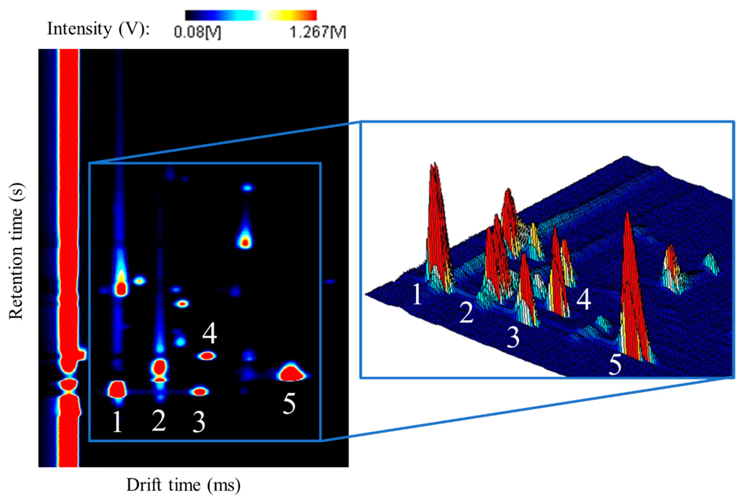
3.2. VOCs Identification

The values of drift time (s), retention (ms) time, and intensity (V) of each analyte were exported from all the spectra. Among monomers, dimers, and even some trimers, 33 peaks were detected. Their identification consisted in crosschecking the exported drift and retention times with the values of the developed database of VOCs. It was possible to successfully identify 22 peaks among the 33 detected. These 22 peaks correspond to 15 VOCs.

Table 2. Detected in the indoor air samples GC-IMS peaks and identified VOCs. Results for each peak are expressed as a mean value of its retention time (in seconds), RIP relative drift time, and normalized ion mobility constant (K₀) based on ten replicate measurements (n = 10).

#	Retention Time (s)	Relative Drift Time	K0	VOCs	CAS Number	Note
1	73.7	1.055	1.990	Ethanol	64-17-5	M
	74.4	1.150	1.826			D
2	84.3	1.104	1.898	2-Propanol	67-63-0	M
	81.3	1.206	1.735			D
	80.9	1.256	1.669			T
3	84.4	1.058	1.985	Propanal	123-38-6	M
4	89.7	1.159	2.080	Acetone	67-64-1	D
	88.7	1.207	1.799			T
5	95.8	1.128	1.861	1-Propanol	71-23-8	M
6	113.2	1.130	1.857	Butanal	123-72-8	M
	113.3	1.334	1.572			D
7	118.6	1.184	1.773	Isobutanol	78-83-1	M
8	119.3	1.060	1.976	Acetic Acid	64-19-7	M
9	119.4	1.120	1.884	Benzene	71-43-2	M
10	123.5	1.081	1.943	2-Butanone	78-93-3	M
	123.2	1.299	1.614			D
11	143.2	1.203	1.757	1-Butanol	71-36-3	M
	140.4	1.425	1.479			D
12	165.6	1.206	1.557	Pentanal	110-62-3	M
13	170.6	1.116	1.886	Propanoic Acid	123-38-6	M
14	252.0	1.285	1.644	Hexanal	66-25-1	M
15	261.3	1.215	1.720	2-Hexanone	107-87-9	M
16	74.0	1.106	1.903	N.I.	-	-
17	96.6	1.056	1.992	N.I.	-	-
18	103.1	1.059	1.986	N.I.	-	-
19	119.3	1.043	2.017	N.I.	-	-
20	123.0	1.227	1.715	N.I.	-	-
21	125.9	1.277	1.648	N.I.	-	-
22	135.0	1.197	1.758	N.I.	-	-
23	139.9	1.340	1.570	N.I.	-	-
24	144.9	1.140	1.846	N.I.	-	-
25	169.9	1.132	1.858	N.I.	-	-
26	261.6	1.706	1.233	N.I.	-	-

summarizes the information regarding the VOCs detected from nine locations. It contains the retention time (s), RIP relative drift time, and the normalized ion mobility constant (K₀) with the indication of monomer (M), a dimer (D), or a trimer (T), as well as CAS number for identified compounds. The unidentified peaks are marked with the acronym N.I. (not identified).

Considering the main reviewed VOCs emitted by both water-based and solvent-based coatings, it was possible to find some matchings among the expected and the identified VOCs, in specific, the compounds 1 (ethanol), 4 (acetone), 5 (propanol), 9 (benzene), and 10 (2-butanone).

Regarding eventual health conditions provoked by exposure to these analytes, ethanol, propanol, acetone, and 2-butanone, for instance, are known for causing extreme irritation and burns in the skin, eyes, nose, and throat. Several other VOCs can also cause reactions of irritation in diverse tissues, namely, 2-propanol, propanal, isobutanol, or acetic acid. Compounds like propanol, 2-butanone, butanal, acetic acid, or isobutanol can be responsible for dizziness, weakness, headaches, breathlessness, chest constriction, and loss of consciousness. Acetone, 2-propanol, and butanol can even induce an anesthetized state, in cases of long-term exposure. Benzene, in its turn, can lead to dizziness, weakness, headaches, breathlessness, nausea, vomiting, and, in extreme cases, coma and possible death. Concisely, all the identified VOCs can have serious impacts on employees’ health. Deeper studies are already being prepared in order to increase the list of identified compounds and evaluate the eventual pathologies promoted by those VOCs.

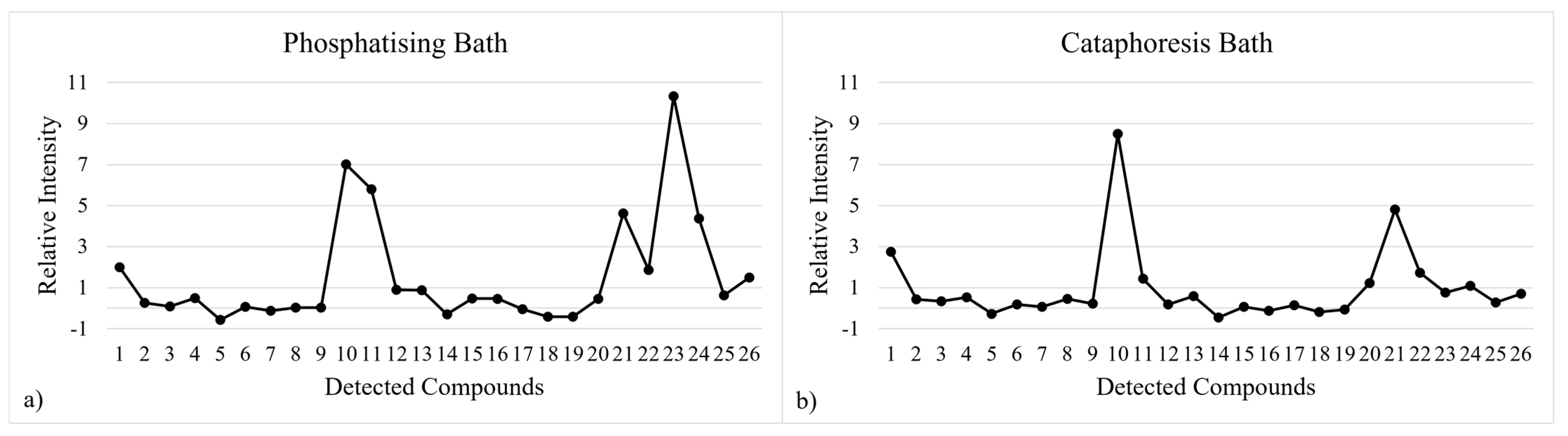
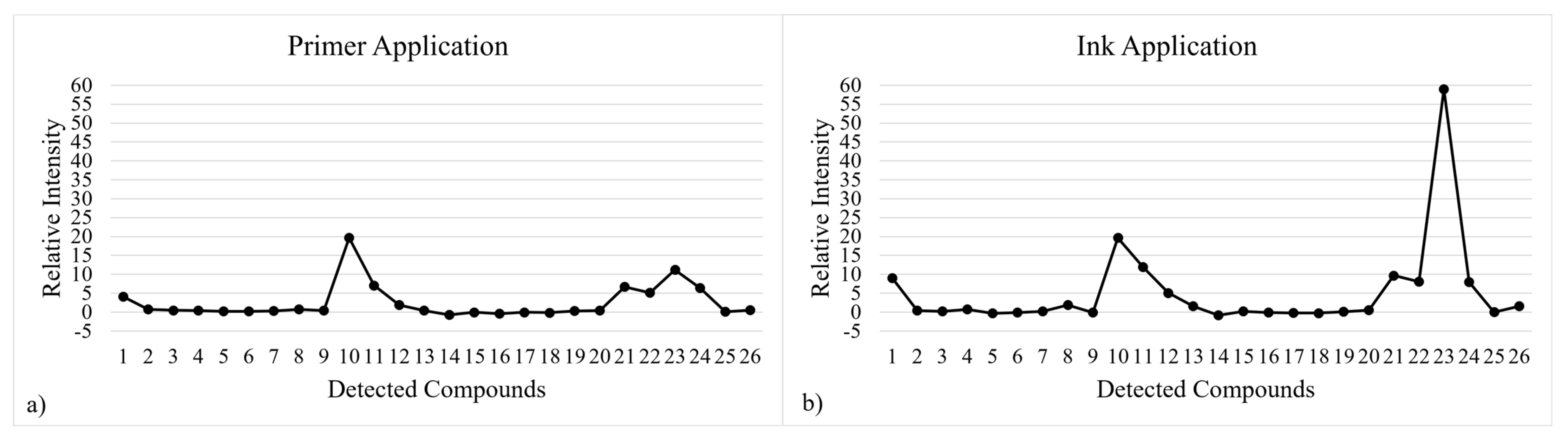
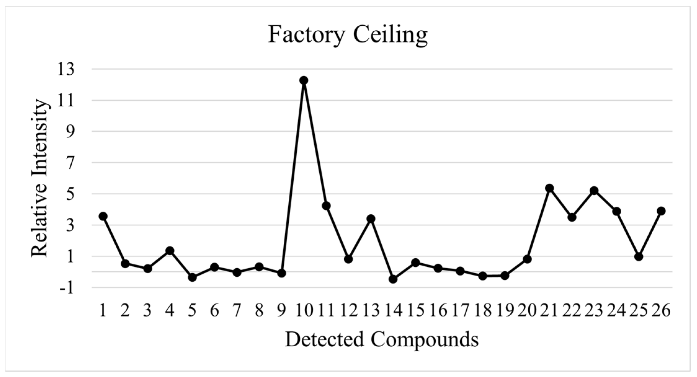
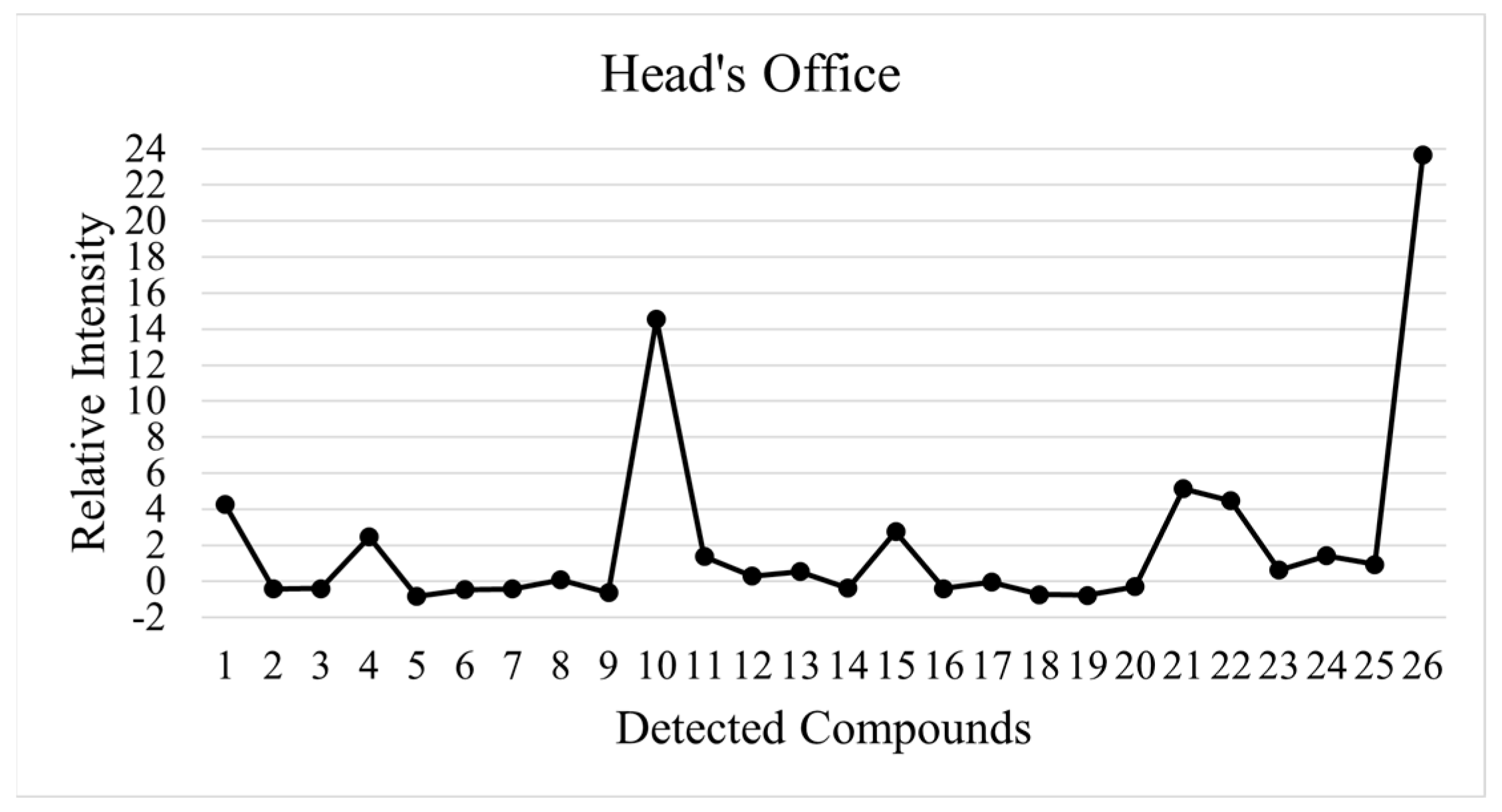
3.3. VOCs Quantification

The third value of the GC-IMS spectra, the intensity, was used for plotting intensity profiles for each location. The intensities of each compound’s monomer, dimer, and trimer were summed, and its average intensity was calculated for all 10 replicates. This procedure was repeated for all 26 detected analytes. Subsequently, the intensity levels of each location were normalized against the outdoor air intensity levels. To do so, the ratio between the average intensity of each VOC, for each location, and the respective intensity value in outdoor air samples was calculated. Thus, the intensity of each compound in outdoor air samples is taken as the zero of reference, meaning that if a compound has a relative intensity value above the reference zero, its intensity is higher in that location than it is outdoors. On the other hand, if that compound has an intensity value under zero, for a specific location, its intensity is lower in this location than it is outdoors. As an example, if ethanol has a relative intensity of two in some random location, this means that its intensity and, consequently, its concentration is two times higher in this location than it is outdoors. The relative intensity profiles were plotted and arranged in five groups considering the characteristics and the proximity between each location. The calculated values of relative intensity and respective standard deviation are summarized in Table S1, available in the Supplementary Materials.

The intensity levels against the outdoor intensity, for the 26 VOCs existing in the phosphatizing bath and cataphoresis bath stages are represented in Figure 5a,b, respectively. As mentioned, both these contiguous stages consist of immersing the car bodies in large reservoirs of chemicals for purposes of metal and surface preparation, so the presence and intensity of VOCs in these locations are relevant topics.

It is possible to discern several similarities and some differences between the profiles. Regarding the similarities, the VOCs 2 (2-propanol) to 9 (benzene) and 12 (pentanal) to 20 (not identified) present, for both profiles, intensity levels that are very close to the outdoor levels since they barely diverge from the zero of reference, meaning that they do not constitute a threat to the employees’ health. However, there are some analytes whose intensities make them of special interest. Compound 10 (2-butanone), for example, is seven and nine times more intense in (a) and (b), respectively, than it is in the outdoor air. Compound 21 (not identified) also presents similar behavior in both locations. It is five times more intense in the indoor air samples than it is in the outdoor samples. These elevated intensities prove that not only is there a very efficient VOC-emitting source in both phosphatizing and cataphoresis baths, but also that the two analytes must be carefully monitored and controlled.

There are some analytes whose elevated intensities are only visible in the profile of the phosphatizing bath, namely, compounds 11 (butanol), 23 (not identified), and 24 (not identified). These analytes are eleven, five, and three times more intense in the phosphatizing bath location than they are outside. For this reason, they have to be identified and their concentration levels must be assessed in order to evaluate the eventual impacts on the employees’ health. If proven necessary, the extraction systems have to be modified and improved.

The processes of primer and ink application to the metal surface of the car body are also contiguous and the central stages of the entire painting line. Both of them are performed by robotic arms that eject a coating cloud against the metal surface. Figure 6 represents the relative intensity profiles for (a) primer and (b) ink application.

Differently from the previous group of profiles, here, the differences are less evident. It is clear that most volatile organic compounds have relative intensities of around zero, which means that the intensities of these VOCs inside the primer and ink application chambers are very similar to the intensities of the same VOCs in outdoor air samples. This fact can mean that the extraction systems have some positive effects on maintaining the air quality inside the chamber. Despite the controlled VOCs, both profiles have some compounds whose intensity is significantly elevated.

Compound 10 (2-butanone) is twenty times more intense in both primer and ink application locations than it is in the outdoor environment. Similarly, VOC 11 (1-butanol) also has a considerably elevated intensity, specifically, seven and eleven times higher for (a) and (b), respectively, than for the outdoor air. Compounds 21 (not identified), 22 (not identified), and 24 (not identified) present the same relative intensities in both (a) and (b) locations; they are five times more intense in both primer and ink application than they are in the outdoor air. All these analytes must be carefully controlled, and their real concentration levels have to be assessed to preserve the integrity of the employees’ health.

A final analyte, compound 23 (not identified), presents a relative intensity close to sixty, meaning that this compound is sixty times more intense in the interior of the ink application chamber than it is in the outdoor air samples. Unfortunately, its identification was not achieved during the development of this work: nonetheless, since its concentration in the air is, potentially, very elevated, it is a mandatory topic to qualitatively and quantitatively assess further details about the analyte and understand what risks and consequences the compound may represent to the workers of the car factory painting line.

Figure 7 represents the relative intensity profiles for the stages of the (a) varnish application and (b) wax application of the painting line. As in the previous two groups of profiles, these two locations are also adjacent, so their comparison is relevant.

As seen in previous scenarios, most of the volatile organic compounds have a relative intensity of around zero. For example, compounds 5 (1-propanol), 6 (butanal), 7 (isobutanol), 8 (acetic acid), and 9 (benzene) have intensities levels close to their intensities in outdoor environments. These are positive results since the compounds do not characterize a significant risk to the health of the workers.

The analytes 1 (ethanol), 21 (not identified), and 22 (not identified) have relative intensity levels of five. Similarly, compound 24 (not identified) presents a relative intensity of seven in the varnish application location, meaning that it is seven times more intense in this indoor location than it is in the outdoor air and, depending on its real concentration, may be potentially hazardous to the employees’ health.

Regarding the most intense analytes, three VOCs must be highlighted. Compound 11 (1-butanol) reaches levels of the relative intensity of five and ten times for the locations of wax application and varnish application, respectively. Compound 10 (2-butanone) behaves similarly. Its relative intensity reaches up to ten and twenty for wax and varnish application, respectively. Finally, the most intense analyte is compound 23 (not identified). Despite having a lower relative intensity in the location of wax application, it is twenty-two times more intense in the indoor air of the varnish application location than it is outside.

All the aforementioned values are worthy of attention so, the identification of the unidentified compounds and the quantification of all 26 analytes are mandatory tasks that must be performed immediately.

The factory ceiling is the location where the main air extraction systems and pipelines are installed; in this way, it was expected to find some diversity of volatile organic compounds in this area. Figure 8 represents the relative intensity profile for the measurements performed near the mentioned systems.

Curiously, the relative intensity levels were not as elevated as expected; nevertheless, some analytes still deserve proper and careful attention. Compound 10 (2-butanone), for instance, is the analyte with higher relative intensity; it is almost thirteen times more elevated in air samples collected near the ceiling than it is in outdoor air samples.

The analytes 11 (1-butanone), 21 (not identified), and 23 (not identified) have relative intensities of five. Ethanol (compound 1), propanoic acid (compound 13), and the VOCs 22 (not identified), 24 (not identified), and 26 (not identified), in their turn, have relative intensities of around three. All the mentioned analytes present considerably elevated relative intensity levels; in this way, their eventual impacts on public health must be deeply studied.

Finally, the last analyzed location was the office of the painting line manager. As mentioned, this room is independent and isolated from the painting line so, it was expected to find a distinct behavior of the VOCs’ relative intensity. Figure 9 represents the mentioned profile.

The more relevant volatile organic compounds in this profile are compounds 10 (2-butanone) and 26 (not identified), which are around 14 and 24 times more intense in the interior of the office than they are in the outdoor samples. Compounds 1 (ethanol), 21, and 22 (not identified) have relative intensities between 4 and 6, and compounds 4 (acetone) and 15 (2-hexanone) are two times more intense in the indoor air than outside. These values cannot be ignored, so the addressed VOCs must be deeply assessed in order to evaluate the eventual risks for workers in both scenarios of short- and long-term exposure.

To understand the real hazardousness of the detected analytes and, consequently, assess the real impact on the health of the employees, it is important to know the levels of concentration existent in the analyzed air samples. To do so, a calibration protocol previously developed was applied to our data. Further details regarding the developed methodology can be consulted elsewhere [53,55]; nevertheless, it is important to emphasize the complexity of calibrating the GC-IMS technology. Considering these limitations, which can be consulted in the mentioned literature, the present work reports a calibration for one of the detected VOCs, namely, the 2-hexanone, for exemplificative purposes. The logarithmic curve adjusted for the calibration of 2-hexanone is represented by the equation below, where y corresponds to the intensity levels, in V, and x corresponds to the concentration levels, in ppm_v.

$$y\left(x\right)=3261.8\ln \left(x\right)+12125,$$

(6)

Once the equation is applied to the intensity levels detected by GC-IMS, it was possible to quantify the levels of 2-hexanone existent in the indoor air throughout all the studied locations.

Table 3. Average levels of concentration and respective standard deviation of 2-hexanone throughout all the studied locations.

Locations	Concentration (ppbv)	Standard Deviation (ppbv)
Phosphatizing Bath	26.6	0.2
Cataphoresis Bath	25.9	0.2
Primer Application	25.8	0.2
Ink Application	26.1	0.2
Varnish Application	25.9	0.1
Wax Application	26.9	0.4
Factory Ceiling	26.8	0.4
Head’s Office	30.5	0.9

summarizes the concentration levels of this analyte in parts per billion (ppb_v).

NIOSH defines the TLV of 2-hexanone at 5 ppm_v [17]. Since the levels of concentration calculated for the 2-hexanone are considerably lower than the defined TLV, it is safe to say that this analyte does not constitute a threat to the employees’ health in scenarios of long-term exposure. Nonetheless, it is important to state that 2-hexanone presented levels of intensity in indoor environments not higher than 2 or 3 times its levels outdoors, but other analytes presented relative intensity levels as high as 10, 20, and even 60 times higher than their levels in the outdoor air samples. This fact might mean that the concentrations of these analytes can equally be considerably higher than the 2-hexanone concentrations, which proves the necessity of calibrating all the remaining detected analytes to fully characterize their hazardousness to human health.

4. Conclusions

The present work focused on assessing the Gas Chromatography–Ion Mobility Spectrometry suitability for indoor air evaluation and control in the interior of a car factory painting line. A total of 80 three-dimensional spectra from the eight main stages of the painting line were analyzed. Among the 33 detected peaks corresponding to 26 analytes, 15 volatile organic compounds were successfully identified. Considering the information gathered about the expected VOCs to be emitted from primer, ink, varnish, and other chemical-based solutions used during the work shifts, it was possible to conclude that 5 of the 15 identified VOCs belong to the list of anticipated VOCs, namely, ethanol, acetone, propanol, benzene, and 2-butanone. Some of these compounds have been described in the literature as being directly responsible for several health conditions and pathologies like eye allergies, skin irritation, liver and kidney conditions, and even lung and other types of cancers. In addition, the remaining identified analytes are equally known for causing several health conditions in both short- and long-term exposure scenarios.

Relative intensity profiles were plotted for all eight analyzed locations. For this, the intensity of a compound’s monomer, dimer, and trimer was summed and then the intensity values relative to the outdoor air samples were estimated; i.e., the intensity values were normalized in relation to the outdoor levels. This approach enabled the authors to realize that some VOCs were 5, 10, 25, and even 60 times more intense in the indoor air of the studied environments, specifically, inside the painting line stages, than they were in the outdoor air samples.

Concentration levels were calculated for one of the detected analytes, 2-hexanone, by applying a previously developed logarithmic model developed for calibrating the relationship between the levels of intensity detected by the GC-IMS and the concentration of the analyte in the original sample. The quantification of 2-hexanone was accomplished in the range of tens of part-per-billions, which demonstrates that at least this analyte does not represent a direct threat to the health of the employees.

In summary, the obtained results show a good analytical precision of the proposed method for sampling and analysis of volatile organic compounds in trace concentrations. Regarding the analytical technique used for this study, which was used for the first time in an automotive factory, GC-IMS proved to be suitable for indoor air analysis and online VOC detection in real industrial scenarios. Its high selectivity, sensitivity, and analytical flexibility allied with its portability, and in loco measurement capacity characterize GC-IMS as the most adequate technique for the scope and goals of this project.

It is important, nonetheless, to reinforce the necessity of overcoming the limitations of this technology. As addressed, the lack of certified databases of VOCs is a major limitation of the employed technique since it hardens the accurate identification of the detected analytes and the proper quantification of the intensity levels. These limitations prevent us from fully assessing the impacts of the VOCs on employees, whose work conditions deserve full attention. To overcome these issues, additional techniques with certified libraries can be employed, enabling an accurate qualification and quantification of all the detected analytes, namely, spectroscopic/spectrometric- and chromatographic-based technologies. In addition, biomonitoring studies should be implemented to correctly assess the real impacts on employees’ health of exposure to hazardous analytes.

The achieved results confirmed the necessity of developing deeper studies to identify the remaining VOCs, increase the VOC database, quantify all the detected analytes, and, consequently, evaluate their hazardousness to the employees’ health. Analyzing all the chemical-based products, namely, primer, ink, varnish, and wax, among others, must also be considered. The utilization of additional techniques, preferably, with certified libraries available, should be considered.

References

1. Bruice, P.Y. Organic Chemistry, 8th ed.; Pearson Education: Hoboken, NJ, USA, 2016. [Google Scholar]
2. Carey, F.A.; Giuliano, R.M. Organic Chemistry, 11th ed.; McGraw-Hill Education: New York, NY, USA, 2017. [Google Scholar]
3. Klein, D. Organic Chemistry, 3rd ed.; John Wiley and Sons, Inc.: Hoboken, NJ, USA, 2017. [Google Scholar]
4. Solomons, T.W.G.; Fryhle, C.B. Organic Chemistry, 12th ed.; John Wiley & Sons, Inc.: Hoboken, NJ, USA, 2009. [Google Scholar]
5. European Union. Directive 2004/42/CE of the European Parliament and of the Council of 21 April 2004 on the limitation of emissions of volatile organic compounds due to the use of organic solvents in certain paints and varnishes and vehicle refinishing products. Off. J. Eur. Union. 2004, 143, 87–96. [Google Scholar]
6. Montero-Montoya, R.; López-Vargas, R.; Arellano-Aguilar, O. Volatile Organic Compounds in Air: Sources, Distribution, Exposure and Associated Illness in Children. Ann. Glob. Health 2018, 84, 225–238. [Google Scholar] [CrossRef] [Green Version]
7. Baurès, E.; Blanchard, O.; Mercier, F.; Surget, E.; Cann, P.; Rivier, A.; Gangneux, J.P.; Florentin, A. Indoor air quality in two French hospitals: Measurement of chemical and microbiological contaminants. Sci. Total Environ. 2018, 642, 168–179. [Google Scholar] [CrossRef]
8. Gallart-Mateu, D.; Armenta, S.; Guardia, M. Indoor and outdoor determination of pesticides in air by ion mobility spectrometry. Talanta 2016, 161, 632–639. [Google Scholar] [CrossRef]
9. Wah, C.; Yu, F.; Kim, J.T. Building Pathology, Investigation of Sick Building—VOC Emissions. Indoor Built Environ. 2010, 19, 30–39. [Google Scholar]
10. Kagi, N.; Fujii, S.; Tamura, H.; Namiki, N. Secondary VOC emissions from flooring material surfaces exposed to ozone or UV irradiation. Build. Environ. 2009, 44, 1199–1205. [Google Scholar] [CrossRef]
11. Śmiełowska, M.; Marć, M.; Zabiegala, B. Indoor air quality in public utility environments—A review. Environ. Sci. Pollut. Res. 2017, 24, 11166–11176. [Google Scholar] [CrossRef] [Green Version]
12. Kumar, A.; Singh, B.P.; Punia, M.; Singh, D.; Kumar, K.; Jain, V.K. Assessment of indoor air concentrations of VOCs and their associated health risks in the library of Jawaharlal Nehru University, New Delhi. Environ. Sci. Pollut. Res. 2014, 21, 2240–2248. [Google Scholar] [CrossRef] [PubMed]
13. Kim, B.R. VOC Emission from Automotive Painting and Their Control: A Review. Environ. Eng. Res. 2011, 16, 1–9. [Google Scholar] [CrossRef]
14. Li, J.; Gutierrez-Osuna, R.; Hodges, R.; Luckey, G.; Crowell, J.; Schiffman, S.; Nagle, H.T. Using Field Asymmetric Ion Mobility Spectrometry for Odor Assessment of Automobile Interior Components. IEEE Sens. J. 2016, 16, 5747–5756. [Google Scholar] [CrossRef]
15. Costello, B.; Amann, A.; Alkateb, H.; Flynn, C.; Filipiak, W.; Khalid, T.; Osborne, D.; Ratcliffe, N. A review of the volatiles from the healthy human body. J. Breath. Res. 2014, 8, 014001. [Google Scholar] [CrossRef]
16. Zhang, R.K.; Wang, J.X.; Cao, H. High-Performance Cataluminescence Sensor Based on Nanosized V2O5 for 2-Butanone Detection. Molecules 2020, 25, 3552. [Google Scholar] [CrossRef]
17. The National Institute for Occupational Safety and Health (NIOSH), Centers for Disease Control and Prevention. Available online: https://www.cdc.gov/niosh/idlh/intridl4.html (accessed on 20 March 2023).
18. Mochalski, P.; Wiesenhofer, H.; Allers, M.; Zimmermann, S.; Guntner, A.T.; Pineau, N.J.; Lederer, W.; Agapiou, A.; Mayhew, C.A.; Ruzsanyi, V. Monitoring of selected skin- and breath-borne volatile organic compounds emitted from the human body using gas chromatography ion mobility spectrometry (GC-IMS). J. Chromatogr. 2018, 1076, 29–34. [Google Scholar] [CrossRef] [Green Version]
19. Haick, H.; Broza, Y.; Mochalski, P.; Ruzsanyi, V.; Amann, A. Assessment, origin, and implementation of breath volatile cancer markers. Chem. Soc. Rev. 2013, 43, 1423–1449. [Google Scholar] [CrossRef] [Green Version]
20. Bessa, V.; Darwiche, K.; Teschler, H.; Sommerwerck, U.; Rabis, T.; Baumbach, J.I.; Freitag, L. Detection of volatile organic compounds (VOCs) in exhaled breath of patients with chronic obstructive pulmonary disease (COPD) by ion mobility spectrometry. Int. J. Ion. Mobil. Spectrom. 2011, 14, 7–13. [Google Scholar] [CrossRef]
21. Handa, H.; Usuba, A.; Maddula, S.; Baumbach, J.I.; Mineshita, M.; Miyazawa, T. Exhaled Breath Analysis for Lung Cancer Detection Using Ion Mobility Spectrometry. PLoS ONE 2014, 9, e114555. [Google Scholar] [CrossRef]
22. Santos, P.H.C.; Vassilenko, V.; Moura, P.C.; Conduto, C.; Fernandes, J.M.; Bonifácio, P. Instrumentation for differentiation of exhaled air. In Proceedings of the Fifteenth International Conference on Correlation Optics, Chernivtsi, Ukraine, 16 September 2021; p. 121262L. [Google Scholar]
23. Szczurek, A.; Maziejuk, M.; Maciejewska, M.; Pietrucha, T.; Sikora, T. BTX compounds recognition in humid air using differential ion mobility spectrometry combined with a classifier. Sens. Actuators B Chem. 2017, 240, 1237–1244. [Google Scholar] [CrossRef]
24. Crump, D.R.; Squire, R.W.; Yu, C.W.F. Sources and Concentrations of Formaldehyde and Other Volatile Organic Compounds in the Indoor Air of Four Newly Built Unoccupied Test Houses. Indoor Built Environ. 1997, 6, 45–55. [Google Scholar] [CrossRef]
25. Xie, Z.; Sielemann, H.; Li, F.; Baumbach, J.I. Determination of acetone, 2-butanone, diethyl ketone and BTX using HSCC-UV-IMS. Anal. Bioanal. Chem. 2002, 372, 606–610. [Google Scholar] [CrossRef]
26. Maziejuk, M.; Szczurek, A.; Maciejewska, M.; Pietrucha, T.; Szyposzynska, M. Determination of benzene, toluene and xylene concentration in humid air using differential ion mobility spectrometry and partial least squares regression. Talanta 2016, 152, 137–146. [Google Scholar] [CrossRef]
27. Lerner, J.E.C.; Sanchez, E.Y.; Sambeth, J.E.; Porta, A.A. Characterization and health risk assessment of VOCs in occupational environments in Buenos Aires, Argentina. Atmos. Environ. 2012, 55, 440–447. [Google Scholar] [CrossRef]
28. Bysko, S.; Krystek, J.; Bysko, S. Automotive Paint Shop 4.0. Comput. Ind. Eng. 2020, 139, 105546. [Google Scholar] [CrossRef]
29. Singgih, I.K.; Yu, O.; Kim, B.; Koo, J.; Lee, S. Production scheduling problem in a factory of automobile component primer painting. J. Intell. Manuf. 2020, 31, 1483–1496. [Google Scholar] [CrossRef]
30. Salihoglu, G.; Salihoglu, N.K. A review on paint sludge from automotive industries: Generation, characteristics and management. J. Environ. Manag. 2016, 169, 223–235. [Google Scholar] [CrossRef]
31. Baumann, W.; Dinglreiter, U. Method for reprocessing and recycling of aqueous rinsing liquids from car painting with water-based paints in automobile industry. Heat. Mass. Transf. 2011, 47, 1043–1049. [Google Scholar] [CrossRef]
32. Moura, P.C.; Raposo, M.; Vassilenko, V. Breath Volatile Organic Compounds (VOCs) as Biomarkers for the Diagnosis of Pathological Conditions: A Review. Biomed. J. 2023, 46, 100623. [Google Scholar] [CrossRef]
33. Günzler, H.; Williams, A. Handbook of Analytical Techniques, 1st ed.; WILEY-VCH Verlag GmbH: Weinheim, Germany, 2001. [Google Scholar]
34. Paglia, G.; Astarita, G. Ion Mobility—Mass Spectrometry, 1st ed.; Humana Press: Totowa, NJ, USA; Springer: New York, NY, USA, 2020. [Google Scholar]
35. Moura, P.C.; Pivetta, T.P.; Vassilenko, V.; Ribeiro, P.A.; Raposo, M. Graphene Oxide Thin Films for Detection and Quantification of Industrially Relevant Alcohols and Acetic Acid. Sensors 2023, 23, 462. [Google Scholar] [CrossRef]
36. Eiceman, G.A.; Karpas, Z.; Hill, H.H. Ion Mobility Spectrometry, 3rd ed.; CRC Press: Boca Raton, FL, USA; Taylor & Francis Group: New York, NY, USA, 2014. [Google Scholar]
37. Moura, P.C.; Vassilenko, V. Contemporary ion mobility spectrometry applications and future trends towards environmental, health and food research: A review. Int. J. Mass. Spectrom. 2023, 486, 117012. [Google Scholar] [CrossRef]
38. Santos, P.; Vassilenko, V.; Conduto, C.; Fernandes, J.M.; Moura, P.C.; Bonifácio, P. Pilot Study for Validation and Differentiation of Alveolar and Esophageal Air. In Proceedings of the Technological Innovation for Applied AI Systems, Doctoral Conference on Computing, Electrical and Industrial Systems (DoCEIS 2021), Caparica, Portugal, 7–9 July 2021. [Google Scholar]
39. Kanu, A.B.; Hill, H.H. Ion mobility spectrometry detection for gas chromatography. J. Chromatogr. A 2008, 1177, 12–27. [Google Scholar] [CrossRef]
40. Santos, F.J.; Galceran, M. The application of gas chromatography to environmental analysis. Trends Anal. Chem. 2002, 21, 672–685. [Google Scholar] [CrossRef]
41. Daris, R.; St-Pierre, C. Beta decay of tritium. Nucl. Phys. A 1969, 138, 545–555. [Google Scholar] [CrossRef]
42. Kuklya, A.; Reinecke, T.; Uteschil, F.; Kerpen, K.; Zimmermann, S.; Telgheder, U. X-ray ionization differential ion mobility spectrometry. Talanta 2017, 162, 159–166. [Google Scholar] [CrossRef]
43. Wilkins, C.L.; Trimpin, S. Ion Mobility Spectrometry—Mass Spectrometry, 1st ed.; CRC Press: Boca Raton, FL, USA; Taylor & Francis Group: New York, NY, USA, 2011. [Google Scholar]
44. Hill, H.H.; Siems, W.F.; Louis, R.H.S.; McMinn, D.G. Ion Mobility Spectrometry. Anal. Chem. 1990, 62, 1201–1209. [Google Scholar] [CrossRef]
45. Kaur-Atwal, G.; O’Connor, G.; Aksenov, A.A.; Bocos-Bintintan, V.; Thomas, C.L.P.; Creaser, C.S. Chemical standards for ion mobility spectrometry: A review. Int. J. Ion. Mobil. Spectrom. 2009, 12, 1–14. [Google Scholar] [CrossRef]
46. Krylov, E.; Nazarov, E.G.; Miller, R.A.; Tadjikov, B.; Eiceman, G.A. Field dependence of mobilities for gas-phase-protonated monomers and proton-bound dimers of ketones by planar field asymmetric waveform ion mobility spectrometer (PFAIMS). J. Phys. Chem. 2002, 106, 5437–5444. [Google Scholar] [CrossRef]
47. Moura, P.C.; Vassilenko, V. Gas Chromatography—Ion Mobility Spectrometry as a tool for quick detection of hazardous volatile organic compounds in indoor and ambient air: A university campus case study. Eur. J. Mass. Spectrom. 2022, 28, 113–126. [Google Scholar] [CrossRef]
48. Moura, P.C.; Vassilenko, V.; Fernandes, J.M.; Santos, P.H. Indoor and Outdoor Air Profiling with GC-IMS. In Proceedings of the Technological Innovation for Life Improvement, Doctoral Conference on Computing, Electrical and Industrial Systems (DoCEIS 2020), Caparica, Portugal, 1–3 July 2020. [Google Scholar]
49. Creaser, C.S.; Griffiths, J.R.; Bramwell, C.J.; Noreen, S.; Hill, C.A.; Thomas, C.L.P. Ion mobility spectrometry: A review. Part 1. Structural analysis by mobility measurement. Analyst 2004, 129, 984–994. [Google Scholar] [CrossRef]
50. Borsdorf, H.; Eiceman, G.A. Ion Mobility Spectrometry: Principles and Applications. Appl. Spectrosc. Rev. 2006, 41, 323–375. [Google Scholar] [CrossRef]
51. Ewing, R.G.; Atkinson, D.A.; Eiceman, G.A.; Ewing, G.J. A critical review of ion mobility spectrometry for the detection of explosives and explosive related compounds. Talanta 2001, 54, 515–529. [Google Scholar] [CrossRef]
52. Gabelica, V.; Marklund, E. Fundamentals of ion mobility spectrometry. Curr. Opin. Chem. Biol. 2018, 42, 51–59. [Google Scholar] [CrossRef] [Green Version]
53. Moura, P.C.; Vassilenko, V.; Ribeiro, P.A. Ion Mobility Spectrometry Towards Environmental Volatile Organic Compounds Identification and Quantification: A Comparative Overview over Infrared Spectroscopy. Emiss. Control Sci. Technol. 2023, 9, 25–46. [Google Scholar] [CrossRef]
54. Puton, J.; Holopainen, S.I.; Mäkinen, M.A.; Sillanpää, E.T. Quantitative Response of IMS Detector for Mixtures Containing Two Active Components. Anal. Chem. 2012, 84, 9131–9138. [Google Scholar] [CrossRef]
55. Fernandes, J.M.; Vassilenko, V.; Moura, P.C.; Fetter, V. Gas Chromatography—Ion Mobility Spectrometry Instrument for Medical Applications: A Calibration Protocol for ppb and ppt Concentration Range. In Proceedings of the Technological Innovation for Applied AI Systems, Doctoral Conference on Computing, Electrical and Industrial Systems (DoCEIS 2021), Caparica, Portugal, 7–9 July 2021. [Google Scholar]
Figure 1. Main steps of the coating process in a car factory painting line.
Processes 11 02259 g001
Figure 2. Example of a three-dimensional spectrum produced after an IMS analysis, in which some VOCs are identified for elucidative purposes (1—monomer of ethanol, 2—monomer of 2-propanol, 3—dimer of ethanol, 4—monomer of acetone, and 5—dimer of 2-propanol).
Processes 11 02259 g002
Figure 3. Procedure for collecting the air samples with a Teflon container.
Processes 11 02259 g003
Figure 4. Repeatability graph for the retention time (a), the relative drift time (b), and the normalized intensity (c) for ten samples of a randomly selected analyte (dimer of acetone) analyzed with the GC-IMS.
Processes 11 02259 g004
Figure 5. Relative intensity profiles achieved for (a) phosphatizing bath and (b) cataphoresis bath locations.
Processes 11 02259 g005
Figure 6. Relative intensity profiles achieved for (a) primer application and (b) ink application locations.
Processes 11 02259 g006
Figure 7. Relative intensity profiles achieved for (a) varnish application and (b) wax application locations.
Processes 11 02259 g007
Figure 8. Relative intensity profiles achieved for factory ceiling location.
Processes 11 02259 g008
Figure 9. Relative intensity profiles achieved for head office location.
Processes 11 02259 g009