Article

Numerical Simulation of Optimized Step-Wise Depressurization for Enhanced Natural Gas Hydrate Production in the Nankai Trough of Japan

1
Key Laboratory of Ocean Energy Utilization and Energy Conservation, Ministry of Education, School of Energy and Power Engineering, Dalian University of Technology, Dalian 116024, China
2
School of Mechanical and Power Engineering, Dalian Ocean University, Dalian 116023, China
*
Authors to whom correspondence should be addressed.
Processes 2023, 11(6), 1812; https://doi.org/10.3390/pr11061812
Submission received: 25 May 2023 / Revised: 8 June 2023 / Accepted: 12 June 2023 / Published: 14 June 2023
(This article belongs to the Special Issue Production of Energy-Efficient Natural Gas Hydrate)

Abstract

:
The utilization of natural gas hydrates as an alternative energy source has garnered significant attention due to their proven potential. Despite the successful offshore natural gas hydrate production tests, commercial exploitation has not been achieved. This study aims to enhance the understanding of gas production behavior through simulations from a single vertical well in the Nankai Trough and assess the effectiveness of the step-wise depressurization method for gas production using TOUGH + HYDRATE. The simulation results showed that the effective permeability for the water phase decreased as the hydrates were decomposed, and the invasion of the pore water from the underburden eliminated this effect. Compared with the direct depressurization method, the step-wise depressurization method significantly increased the cumulative gas production by more than 10% and mitigated the rapid generation of gas and water production during the moment of depressurization. The results also indicated that the depressurization gradient was more sensitive to the cumulative gas production than the maintenance time of depressurization. In view of the gas and water production characteristics coupled with the challenges in carrying out the step-wise depressurization method, it is suggested that a depressurization gradient of 1 MPa and a maintenance time of 1 day should be employed.

1. Introduction

Natural gas hydrates (NGHs) are crystalline solid, nonstoichiometric compounds that form under a special environment of low temperature and high pressure [1,2,3]. They are primarily present in continental slopes, deep-sea, or permanent frozen strata [4,5,6]. They are considered as one of the most promising alternative energy sources due to the characteristics of high energy density, wide distribution, and combustion cleanliness [7,8,9].
The mechanism of the exploitation is to break the phase equilibrium of NGHs and extract gas from the NGH reservoir [10,11]. There are four main exploitation methods, including depressurization, thermal injection, chemical inhibitor injection, and carbon dioxide replacement methods [12,13]. The thermal injection method has poor energy efficiency due to the low energy transformation ratio [14,15]. Environmental concerns and potential reservoir pollution are major problems for the chemical inhibitor injection method [16,17]. The low replacement rate limits the development of the carbon dioxide replacement method [18,19]. Depressurization is generally believed to be the most promising method because of its simplicity, technical feasibility, and economic effectiveness [20,21,22]. Recent offshore NGH field tests conducted by Japan and China, during which the depressurization method was used, suggested the possibility of extracting gas from NGH reservoirs [23,24,25,26]. In 2013, Japan conducted the world’s first offshore production test of NGHs using a single vertical well. This test was successful in producing a cumulative volume of 119,500 m3 of natural gas over a period of 6 days, with an average daily production rate of 2.0 × 10⁴ m3/d. It is worth noting that the production test lasted only 6 days, primarily due to the severe issue of sand production. In 2017, Japan conducted a second offshore production test of NGHs following the first test in 2013. It was reported that a total of around 2.0 × 10⁵ m3 of natural gas was produced over a period of 24 consecutive days (i.e., 8.33 × 10³ m3/d) during this recent test. Additionally, in 2017, China conducted a production test of NGHs in the Shenhu area of the South China Sea, achieving a cumulative gas production of 3.09 × 10⁵ m3 during 60 days with an average production rate of 5.15 × 10³ m3/d. In 2020, China’s second production test of NGHs resulted in an improvement in the average gas production rate, with a cumulative gas production of 8.614 × 10⁵ m3 over 30 days and an average production rate of 2.87 × 10⁴ m3/d. However, the issue of sand production remains a significant concern and the gas production rates of the recent field tests were far from the commercial exploration level of 5.0 × 10⁵ m3/d (0.1 MPa and 289 K) [2]. Consequently, in order to achieve successful commercial gas production from offshore NGH deposits in the future, significant improvements in production efficiency are necessary, and the depressurization method must be optimized [27].
Numerous laboratory-scale studies have investigated the optimization of depressurization method for the development of the offshore NGH deposits, including the step-wise depressurization method. For example, Heeschen et al. [28] compared the effects of two gradient depressurization modes, 7.0-5.0-4.2 MPa and 9.0-7.0-5.0-4.2-3.0 MPa, on gas production behaviors using the gas production test results of Mallik as a basis. The results showed that the second mode with a small depressurization gradient had a higher cumulative gas yield. Yang et al. [29] used real marine sediments as a carrier to compare and study the production behaviors of natural gas by single-step and multi-step decompression methods and found that the multi-step method could alleviate the reservoir temperature drop. Zhao et al. [30] employed a multi-level pressure reduction approach in their study of hydrate exploitation and found that it could effectively mitigate the reservoir temperature decline. In addition, a small depressurization gradient of 0.5 MPa could increase the rate of hydrate decomposition by 18.92%. Overall, at the laboratory scale, the step-wise depressurization method may potentially improve the rate of hydrate decomposition and the cumulative gas production.
Due to the difficulties and exorbitant costs associated with field testing, the study of reservoir-scale phenomena is often carried out using numerical simulations. These simulations prove useful in determining the most efficient exploitation methods and monitoring changes in reservoir characteristics. Several specialized simulators, such as TOUGH + HYDRATE, STOMP-HYD, CMG-STARS, and MH21-HYDRES, have been developed for this purpose. Utilizing the field test data, numerous numerical simulations have been conducted to enhance gas productivity, including the utilization of horizontal wells, hot water injection, gas exchange, and permeability enhancement techniques of the NGH reservoirs. However, research on the step-wise depressurization method for gas production at the reservoir scale remains limited.
The main objective of this study was to investigate the effects of different step-wise depressurization methods on natural gas hydrate production in the Nankai Trough of Japan and identify the optimal depressurization strategy. To achieve this aim, a multi-layered NGH reservoir model was established, which provided a more accurate representation of the reservoir conditions compared to a single-layered model. The accuracy of the model was confirmed through the comparison with the actual field test data. Then, the gas and water production characteristics and changes in reservoir permeability over the course of one year were analyzed in this study. Ten scenarios were simulated to evaluate the effects of the key factors, such as the depressurization gradient and maintenance time after each depressurization step, on gas and water production. The cumulative gas and water production from different step-wise depressurization cases were also compared after 100 d of production. Additionally, the evolution of reservoir characteristics distribution by the step-wise depressurization method had also been presented in this study. The results of this research are expected to provide valuable guidance for future commercial NGH production initiatives.

2. Numerical Modeling

2.1. Numerical Simulator

The TOUGH + HYDRATE software developed by the Lawrence Berkeley National Laboratory is widely used for simulating gas production behaviors in NGH reservoirs [31]. This simulator has a good track record of accurate predictions, as confirmed by many scholars [4,32,33]. This simulator was also employed for predicting gas and water production in this study. Specifically, the equilibrium model was adopted, and all the simulation results were obtained based on the assumption that sand production has been fully controlled and the pore structure of the NGH reservoirs would not be deformed. The main control equations are the mass and energy balance equations as follows,
d d t V n M κ d V = Γ n F κ · n d Γ + V n q κ d V ,
where M κ , F κ , and q κ represent the mass accumulation term, Darcy flux vector, and source or sink term, respectively; V n , Γ n , and κ represent the grid volume (m3), grid surface area (m2), and component, respectively; t represents time (s); and V and Γ are the volume (m3) and surface area (m2), respectively.

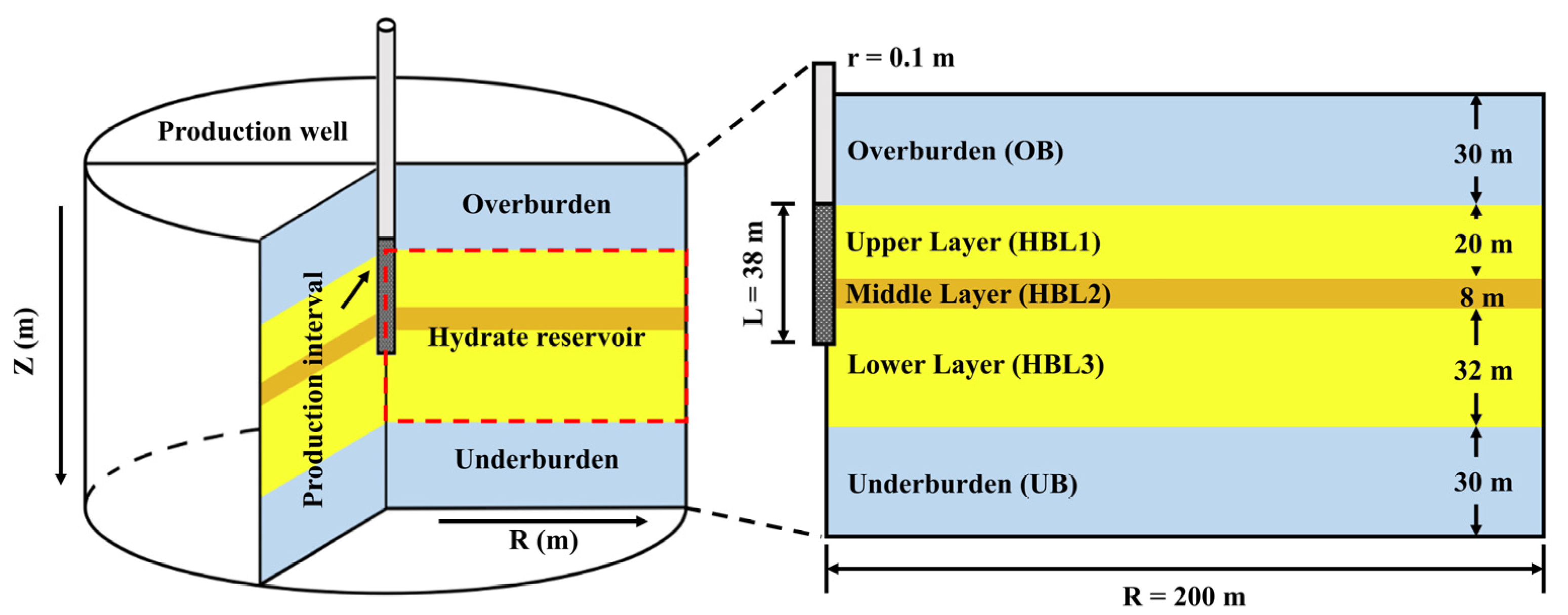
2.2. Model Construction and Domain Discretization

The production site AT1 in the Nankai Trough was chosen for the simulations. This site is located in the Daini Astumi Knoll of the Eastern Nankai Trough off the Pacific coast of Japan [24]. The NGH reservoir at this site comprise upper alternate layers consisting primarily of interbedded sand and silt, middle silt-dominated layers containing mostly silt with sand as the minor component, and lower sand-dominated layers composed primarily of thick sand sequences with little silt [22,24].
A multi-layered NGH reservoir model was utilized in this study, as depicted in Figure 1, which was constructed using a cylindrical coordinate system. The reservoir model was divided into three main sections, the overburden (OB), hydrate layer, and underburden (UB). The hydrate layer was further divided into three sublayers, the upper layer (HBL1), middle layer (HBL2), and lower layer (HBL3), corresponding to the three hydrate sublayers mentioned previously. The OB and UB were set to be 30 m thick, which has been shown to effectively eliminate the boundary effects [34]. The thicknesses of the HBL1, HBL2, and HBL3 were set to be 20 m, 8 m, and 32 m, respectively. The radial extent of the reservoir model was set to be 200 m. A production well with a length of 38 m and a radius of 0.1 m was used in this simulation and positioned in the HBL1 and HBL2 zones, as well as the upper part of the HBL3 zone in order to match the field test.
In this model, a fine grid division was performed, yielding a total of 22,648 grids, with 152 grids along the radial coordinate (r) and 149 grids along the vertical coordinate (z). To ensure efficient calculation while preserving accuracy in predictions, the radial grid size was determined using logarithmic growth. It is noteworthy that the first and last grids along the radial coordinate were set to be 0.1 m to represent the wellbore from which gas and water were produced and the boundary of the model, respectively. The reaction in the hydrate layer is complex, including intricate transformations in heat conduction, hydrate decomposition, and fluid flow. To properly capture these processes, the vertical grid size for the hydrate layer was set to be 1 m, whereas the vertical grid size for the non-hydrate layer was set to be 3 m. Furthermore, to ensure an accurate representation of the reaction, the grids were meticulously fine-tuned at the interface between the layers.

2.3. Initial and Boundaries Conditions

The pressure gradient of the model was assumed to be the hydrostatic pressure gradient and calculated by the empirical formula [35],
P p w = P a t m + ρ s w g ( H + Z ) 10 6 ,
where P p w represents the hydrostatic pore water pressure and P a t m represents the standard atmospheric pressure, MPa; ρ s w is the average seawater density, kg/m3; g stands for the gravitational acceleration, m/s2; H is the water depth, m; and Z is the depth of the sediment from the seafloor, m.
The temperature distribution was derived according to the geothermal gradient and the mean seafloor temperature as follows [22],
T = T s f + Δ T Z × 10 3 ,
where T s f represents the mean temperature of the sea floor, and the value is set to be 3.5 °C according to the literature [24]; Δ T is the geothermal gradient, and the value was set to be 30.0 °C/km. In this simulation, a set of parameters based on relevant studies were used to model the reservoir, such as the porosity, initial hydrate saturation, and intrinsic permeability of each layer [10,36,37]. For example, (a) the porosity was set to be 0.40 for the whole reservoir; (b) the initial hydrate saturations of the HBL1, HBL2, and HBL3 were set to be 0.50, 0.35, and 0.60, respectively; (c) the intrinsic permeability of the reservoir was considered in relation to anisotropy, i.e., the permeabilities in the horizontal and vertical directions of the HBL1, HBL2, and HBL3 were set to be 0.30 D and 0.20 D, 0.05 D and 0.05 D, and 0.40 D and 0.30 D, respectively. The permeability of the OB and UB were set to be isotropic, with the values of 0.01 D and 1.00 D, respectively. The parameters of each layer in this model are listed in Table 1, and the reservoir parameters and conditions used in the simulations are shown in Table 2.
In order to implement the first-type boundary conditions, also known as Dirichlet boundary conditions, fixed pressure and temperature were imposed at the top and bottom of the model. The wellbore pressure was set to be 4.5 MPa, which aligned with the production pressure observed in the field. As depicted in Figure 2, after a prolonged simulation, the formation conditions remained stable, indicating that the model was successfully constructed.

3. Direct Depressurization Method

In this section, the accuracy of the model was verified by comparing the simulation results with the field data collected during the first test of the Nankai Trough. To further investigate the characteristics of gas and water production, a year-long simulation by the direct depressurization method was conducted.

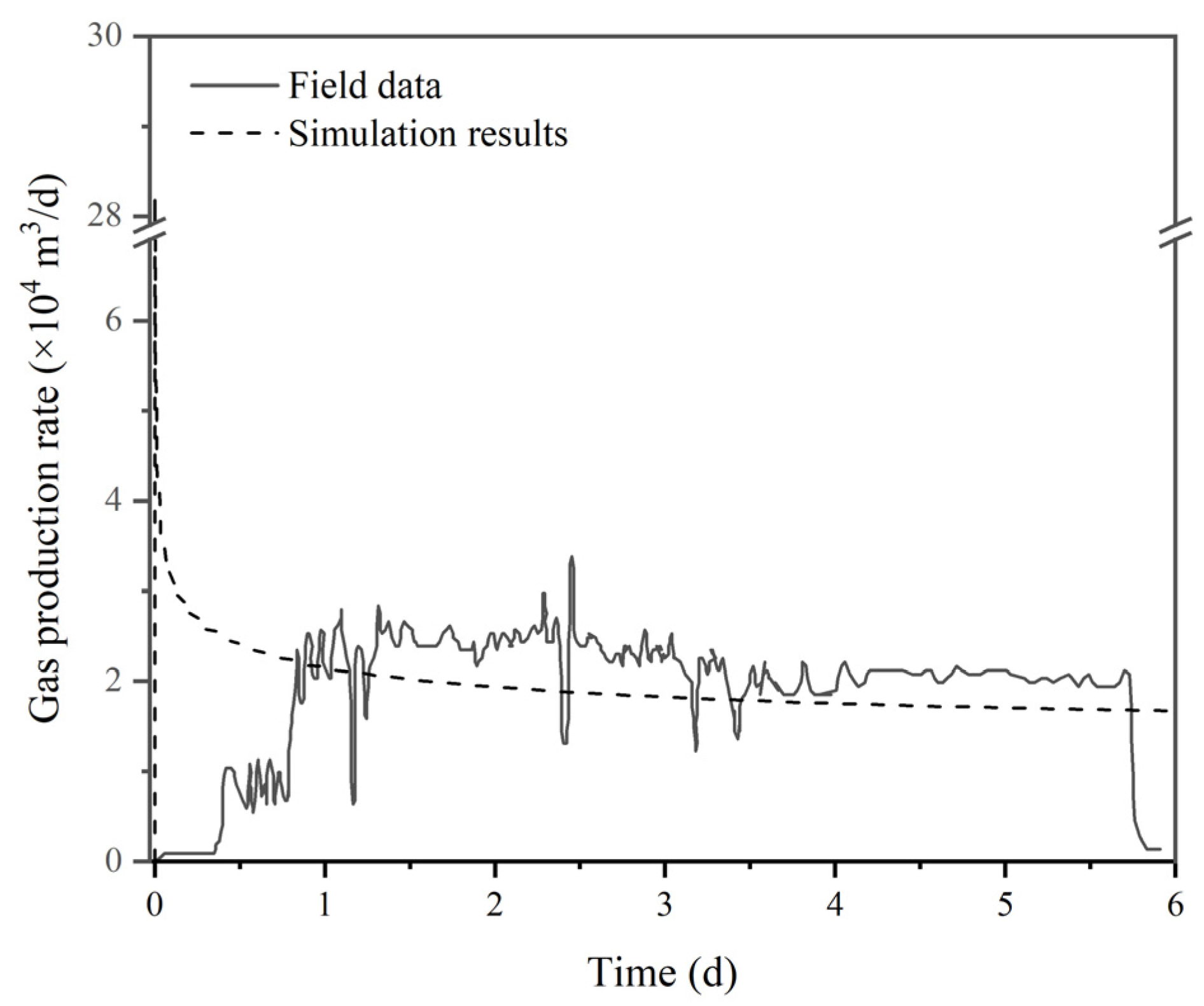
3.1. Model Validation

To ensure the accuracy of the simulations, a 6-day simulation was conducted, as illustrated in Figure 3. The gas production rate remained at approximately 2.0 × 10⁴ m3/d, which was consistent with the field data from the Nankai Trough with the exception of the first day. The unusually high gas production rate on the first day was caused by an instantaneous pressure drop from 13.5 MPa to 4.5 MPa, resulting in a slightly higher cumulative gas production than the actual value. Given the similar results observed in other studies [22,37,40,41], it could be concluded that the model was accurate and has been successfully established. Based on the successful establishment of the model, a one-year simulation by the direct depressurization method was conducted using this model.

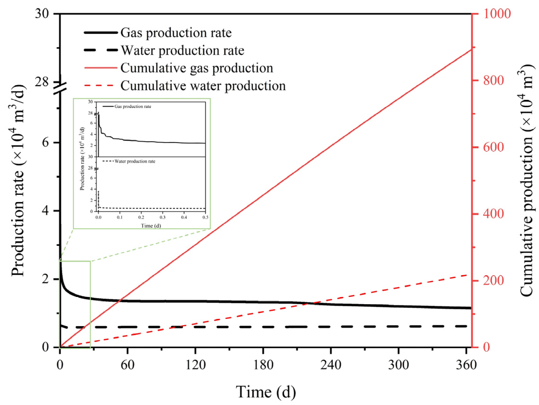
3.2. Characteristics of Gas and Water Production

Figure 4 shows the evolution of gas and water production rates, as well as cumulative gas and water production, during the first year of the simulation. The results indicated that the gas production rate decreased quickly from its initial value of 2.82 × 10⁵ m3/d to approximately 1.6 × 10⁴ m3/d, which was due to the initial sudden pressure drop. The gas production rate then gradually decreased, reaching a value of 1.15 × 10⁴ m3/d at the end of the first year. This decreasing trend was attributed to the slow pressure propagation, which hindered the decomposition of hydrates [41]. In contrast, the water production rate remained stable at 0.6 × 10⁴ m3/d throughout the year. This value was significantly higher than the field test, and this phenomenon was attributed to the use of a waterproof device in the field test that was not accounted for in the simulation.

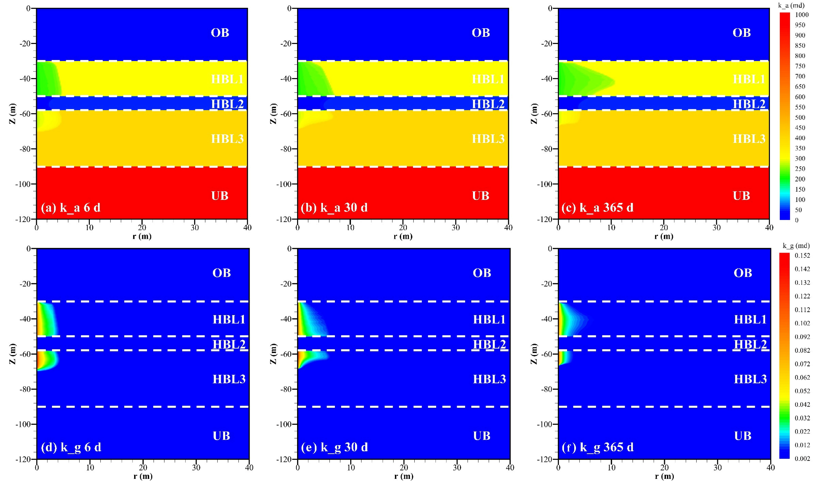
3.3. Evolution of the Reservoir Permeability

Numerous studies have shown that reservoir permeability is a critical factor controlling gas–water flow in reservoirs, which, in turn, is crucial for gas hydrate exploitation. In the TOUGH + HYDRATE simulator, the flowing phase is based on the Darcy’s law and divided into aqueous phase flow and gaseous phase flow, with the effective permeability represented by the rock intrinsic permeability multiplied by the relative permeability of the aqueous/gaseous phase. In this simulation, the modified version of Stone’s three-phase relative permeability method was chosen as the relative permeability model, with specific parameters shown in Table 2. The evolution of effective permeabilities in aqueous and gaseous phase flows are illustrated in Figure 5. During the exploitation process, the effective permeability of the aqueous phase was found to decrease, and the affected area gradually expanded. This phenomenon was beneficial to prevent excessive water production from the production well. The HBL2 was found to exhibit the smallest decrease in effective permeability. Additionally, it was observed that there was no significant decrease in the effective permeability of the aqueous phase in the lower part of the HBL3, hence attention should be paid to the flow of water from the UB into the production well. Regarding the effective permeability of the gaseous phase, it was observed that after gas hydrate decomposition the effective permeability increased, which facilitated the flow of gas into the production well. In addition, the effective permeability decreased as the distance from the production well increased.

4. Optimized Step-Wise Depressurization Method

The direct depressurization method can lead to (a) the emergence of low-temperature zones near the production well [42,43], which negatively impacts the production of nature gas, and (b) large gas and water production in a short time, which may result in sand production issues. In order to address these challenges, a step-wise depressurization method was proposed in this work. To thoroughly and clearly study the effect of the step-wise depressurization method, we have designed 10 sets of cases, each utilizing a different approach to reach a production pressure of 4.5 MPa. Specifically, Case 0 was used as a control group and the direct depressurization method was applied. Cases 1–3, 4–6, and 7–9 utilized the depressurization gradients of 3 MPa, 2 MPa, and 1 MPa, respectively, with the maintenance times of 24, 12, and 6 h after each depressurization stage. The schematic diagram of the step-wise depressurization patterns was shown in Table 3. Additionally, a summary of the different cases and their comparative analysis, aiming to study various influencing factors, was provided in Table 4. Furthermore, the evolution of the distribution of reservoir characteristics was monitored and presented visually.

4.1. Comparison of the Production Behaviors with Different Depressurization Gradients

The production characteristics of gas and water over a 30-day period for Cases 0–3 are displayed in Figure 6, where Figure 6a–d represents the gas production rate, water production rate, cumulative gas production, and cumulative water production, respectively. It can be observed from Figure 6a,b that each time a depressurization operation was carried out the gas and water production rates increased sharply. The peak gas production rate of Case 0 had reached 28.20 × 10⁴ m3/d, while those for Cases 1, 2, and 3 of the step-wise depressurization patterns were 10.52 × 10⁴ m3/d, 7.80 × 10⁴ m3/d, and 5.28 × 10⁴ m3/d, respectively. It was evident that the step-wise depressurization method reduced the sudden large surge in gas production rate from the direct depressurization method by breaking it down into multiple smaller surges. Compared to Case 0, the peak gas production rate of Case 3 decreased by 81.38%. Furthermore, when each step-wise depressurization pattern reached the final production pressure, the gas production rate was higher than that of the direct depressurization method. In terms of water production rate, Case 0 had a peak water production rate of 3.63 × 10⁴ m3/d, whereas those for Cases 1, 2, and 3 of the step-wise depressurization patterns were 1.61 × 10⁴ m3/d, 1.30 × 10⁴ m3/d, and 0.98 × 10⁴ m3/d, respectively. It can be understood that when the water production rate was high, it is easy for sand to be carried along and flow toward the production well. Therefore, it is necessary to avoid such a situation, and the step-wise depressurization method could be used to mitigate this problem to some extent. Case 3, in particular, showed a decrease of 84.02% in peak water production rate compared to Case 0. The cumulative gas and water production of Cases 0–3 are shown in Figure 6c,d. It can be observed that the cumulative gas production of the step-wise depressurization method was higher than that of the direct depressurization method, which confirmed the conclusion drawn from Figure 6a that the gas production rate of the step-wise depressurization method was higher than that of the direct depressurization method. When the gradient of the step-wise depressurization pattern was 1 MPa (Case 3), the increase in cumulative gas production became less significant compared to Case 2. As is well known, water production increases with the increase in gas production [44,45,46]; however, in Case 3, the cumulative water production was not as high as that in Case 2. This could be attributed to the small pressure gradient during each depressurization stage, which resulted in a weaker stimulation of water flow and a slower influx into the production well. In general, the smaller the gradient in the multi-stage depressurization pattern becomes, the more favorable it is for gas production.

4.2. Comparison of the Production Behaviors with Different Maintenance Times

The previous section focused on the impact of the depressurization gradient on the production behavior by the step-wise depressurization method. This section will primarily analyze the effect of maintenance time. The gas and water production behaviors are shown in Figure 7. Cases 3, 6, and 9 all feature the same depressurization gradient of 1 MPa, with different maintenance times of 24 h, 12 h, and 6 h, respectively. From Figure 7a, it can be observed that the peak gas production rate of Case 9 (6.10 × 10⁴ m3/d) was slightly higher than that of Case 3 (5.28 × 10⁴ m3/d), and the gas production rates of all the three cases eventually approach a similar value. As shown in Figure 7b, the peak water production rates were almost identical among Cases 3, 6, and 9, with the values of 0.97 × 10⁴ m3/d, 0.97 × 10⁴ m3/d, and 0.98 × 10⁴ m3/d, respectively. This indicated that the peak value of the water production rate was independent of the maintenance time. As shown in Figure 7c, the cumulative gas production of Cases 3, 6, and 9 were 85.8 × 10⁴ m3, 88.9 × 10⁴ m3, and 90.4 × 10⁴ m3, respectively. Compared with Case 3, the cumulative gas production of Case 9 increased by 5.36%, indicating that shortening the maintenance time was beneficial to increase the cumulative gas production. From Figure 7d, it can be observed that the cumulative water production of Case 9 (18.8 × 10⁴ m3) was 5.62% higher than that of Case 3 (17.8 × 10⁴ m3). The increase in gas production was slightly lower than the increase in water production, which was not the desired result. In summary, shortening the maintenance time is beneficial for improving the gas production rate and cumulative gas production, but it may also result in excessive water production.

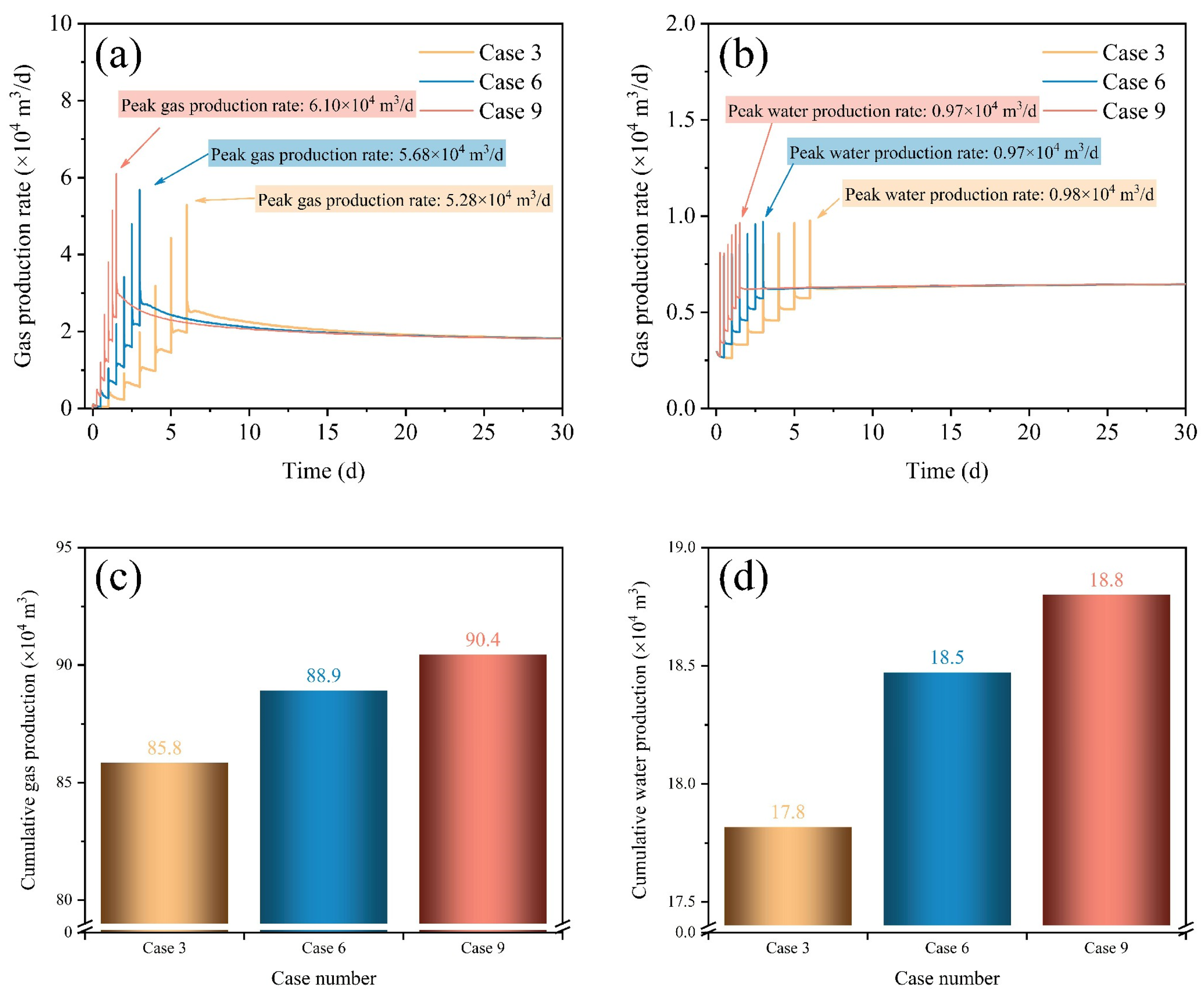
4.3. Comparison of the Cumulative Gas and Water Production for Each Step-Wise Depressurization Pattern

A 100-day simulation was executed to gain a deeper understanding of the effect of the step-wise depressurization method over an extended time frame. The cumulative gas production increment between various step-wise depressurization patterns and the direct depressurization method is depicted in Figure 8. As evidenced, all the step-wise depressurization patterns demonstrated a larger cumulative gas production compared to the direct depressurization method. The cumulative gas production increased as the depressurization gradient decreased and the maintenance time was shortened. The impact of the depressurization gradient on the cumulative gas production surpassed that of the maintenance time on the cumulative gas production. Additionally, it is observed that the cumulative gas production of Case 3 after 100 days was 8.53% higher than that of Case 0, which was even higher than the improvement of 4.63% observed after 30 days (Figure 7). This indicated that the step-wise depressurization method remained effective over a longer period of time. The cumulative water production is shown in Figure 9. It can be observed that the cumulative water production of each case corresponded to its cumulative gas production, with large cumulative gas production being associated with large cumulative water production. Through comparative analyses, it is observed that the increase in cumulative gas production for Case 9 (10.08%) relative to Case 0 was greater than the increase in cumulative water production (8.45%). Through comparison under the same factors, it can be found that compared with Case 1 in terms of depressurization gradient, the cumulative gas production of Case 3 increased by 4.09%, and the cumulative water production increased by 3.10%. Compared with Case 3 in terms of maintenance time, the cumulative gas production of Case 9 increased by 1.43%, and the cumulative water production increased by 1.58%. Therefore, the exploitation conditions used in Case 3 was more favorable for the exploitation of hydrates. In general, step-wise depressurization can alleviate the rapid gas and water production in a short time, and to some extent facilitate the gas exploitation; however, there is still a significant gap between the achieved improvement and commercial exploitation. Thus, it is recommended to combine the step-wise depressurization technique with other methods such as thermal stimulation and permeability enhancement technology for effective exploitation.

4.4. Evolution of Reservoir Characteristics Distribution by Step-Wise Depressurization Method

Considering the comprehensive effects of depressurization gradient and maintenance time on gas and water production, as well as the implementation of step-wise depressurization, it was reasonable to select Case 3 as the optimal production condition. Therefore, Case 3 was chosen for presenting the distribution of reservoir characteristics. The evolution of pressure and temperature at various times (6 d and 30 d) were presented in Figure 10. As observed in Figure 10a,b, the pressure decline was mainly concentrated within a range of 50 m, and the propagation speed of pressure in the HBL2 was slower than those in the other two layers. A small area of low temperature was observed near the production well on the sixth day, as shown in Figure 10c, which could be attributed to the rapid decomposition of hydrates and the Joule–Thomson effect [47]. Additionally, it is observed that the temperature in the lower part of the HBL3 began to increase in Figure 10d. Figure 11 revealed the hydrate and gas saturation distributions in the reservoir. It could be observed that the complete decomposition of gas hydrates occurred within 10 m of the production well. The decomposition rate of gas hydrates in the HBL2 was found to be slower than that of the HBL1 and HBL3, possibly due to the lower permeability of the layer, which hindered the gas–water flow and thus slowed down the decomposition of hydrates. The area of free gas distribution largely overlapped with that of the complete decomposition of gas hydrates. In summary, the evolution of reservoir property distribution by step-wise depressurization exhibited a similar trend to that of direct depressurization [32,41,48]. This similarity could be attributed to the fact that both methods induce gas hydrate decomposition by reducing pressure. However, the step-wise depressurization method yields a larger amount of gas production compared to direct depressurization.

5. Conclusions

In this study, a reservoir model based on the field test results of the Nankai Trough was established, and then a one-year exploitation simulation was conducted for a better understanding of the gas and water production characteristics and the evolution of reservoir characteristics. In addition, the impact of the step-wise depressurization method on the gas extraction from the NGH reservoir was discussed in detail. The main conclusions are as follows:
(1)
The effective permeability for the aqueous phase flow will decrease as the decomposition of gas hydrates, while the pore water flow from other layers will eliminate this effect.
(2)
The step-wise depressurization method is effective in mitigating short-term excessive gas and water production. A small depressurization gradient and a long maintenance time for each stage can enhance the mitigation effect.
(3)
The stepwise depressurization method can increase the cumulative gas production by up to 10% at maximum. Considering the gas and water production characteristics, as well as the difficulty in implementing the step-wise depressurization, it is recommended to adopt a depressurization gradient of 1 MPa and a maintenance time of 1 day.
The simulation results presented in this study primarily focused on evaluating the effectiveness of the step-wise depressurization method for the NGH exploitation in the Nankai Trough of Japan. To provide theoretical support for commercial exploitation, future simulations will be conducted over longer time periods and incorporate various exploitation methods.

Author Contributions

K.X.: Conceptualization, Investigation, Data curation, Writing—original draft; Y.L.: Resources, Funding acquisition, Writing—review and editing; T.Y.: Methodology, Funding acquisition, Writing—review and editing; J.L.: Formal analysis. All authors have read and agreed to the published version of the manuscript.

Funding

This work was supported by the National Natural Science Foundation of China (Grant No. 51976023, 52276053), the National key research and development program (Grant No. 2021YFC2800902) and the Fundamental Research Funds for the Central Universities (Grant No. DUT22LAB115, DUT22RC(3)047).

Data Availability Statement

No new data were created.

Conflicts of Interest

The authors declare that they have no known competing financial interests or personal relationships that could have appeared to influence the work reported in this paper.

References

  1. Collett, T.S.; Johnson, A.H.; Knapp, C.C. Natural Gas Hydrates: A Review. AAPG Mem. 2009, 89, 146–219. [Google Scholar]
  2. Sloan, E.D. Fundamental Principles and Applications of Natural Gas Hydrates. Nature 2003, 426, 353–359. [Google Scholar] [CrossRef]
  3. Boswell, R. Is Gas Hydrate Energy Within Reach? Science 2009, 325, 957–958. [Google Scholar] [CrossRef] [PubMed]
  4. Yin, F.; Gao, Y.; Chen, Y.; Sun, B.; Li, S.; Zhao, D. Numerical Investigation on the Long-Term Production Behavior of Horizontal Well at the Gas Hydrate Production Site in South China Sea. Appl. Energy 2022, 311, 118603. [Google Scholar] [CrossRef]
  5. Lijith, K.P.; Srinivasa Rao, R.; Narain Singh, D. Investigations on the Influence of Wellbore Configuration and Permeability Anisotropy on the Gas Production from a Turbidite Hydrate Reservoir of KG Basin. Fuel 2022, 317, 123562. [Google Scholar] [CrossRef]
  6. Yang, L.; Guan, D.; Qu, A.; Li, Q.; Ge, Y.; Liang, H.; Dong, H.; Leng, S.; Liu, Y.; Zhang, L.; et al. Thermotactic Habit of Gas Hydrate Growth Enables a Fast Transformation of Melting Ice. Appl. Energy 2023, 331, 120372. [Google Scholar] [CrossRef]
  7. Collett, T.S. Energy Resource Potential of Natural Gas Hydrates. AAPG Bull. 2002, 86, 1971–1992. [Google Scholar] [CrossRef] [Green Version]
  8. Li, X.-S.; Xu, C.-G.; Zhang, Y.; Ruan, X.-K.; Li, G.; Wang, Y. Investigation into Gas Production from Natural Gas Hydrate: A Review. Appl. Energy 2016, 172, 286–322. [Google Scholar] [CrossRef] [Green Version]
  9. Makogon, Y.F.; Holditch, S.A.; Makogon, T.Y. Natural Gas-Hydrates—A Potential Energy Source for the 21st Century. J. Pet. Sci. Eng. 2007, 56, 14–31. [Google Scholar] [CrossRef]
  10. Gu, Y.; Sun, J.; Qin, F.; Ning, F.; Cao, X.; Liu, T.; Qin, S.; Zhang, L.; Jiang, G. Enhancing Gas Recovery from Natural Gas Hydrate Reservoirs in the Eastern Nankai Trough: Deep Depressurization and Underburden Sealing. Energy 2023, 262, 125510. [Google Scholar] [CrossRef]
  11. Xue, K.; Liu, Y.; Yu, T.; Yang, L.; Zhao, J.; Song, Y. Numerical Simulation of Gas Hydrate Production in Shenhu Area Using Depressurization: The Effect of Reservoir Permeability Heterogeneity. Energy 2023, 271, 126948. [Google Scholar] [CrossRef]
  12. Song, Y.; Cheng, C.; Zhao, J.; Zhu, Z.; Liu, W.; Yang, M.; Xue, K. Evaluation of Gas Production from Methane Hydrates Using Depressurization, Thermal Stimulation and Combined Methods. Appl. Energy 2015, 145, 265–277. [Google Scholar] [CrossRef]
  13. Wang, Y.; Dong, B.; Zhang, L.; Li, W.; Song, Y. Numerical Simulation of CH4 Recovery from Gas Hydrate Using Gaseous CO2 Injected into Porous Media. J. Nat. Gas Sci. Eng. 2021, 95, 104199. [Google Scholar] [CrossRef]
  14. Jin, G.; Xu, T.; Xin, X.; Wei, M.; Liu, C. Numerical Evaluation of the Methane Production from Unconfined Gas Hydrate-Bearing Sediment by Thermal Stimulation and Depressurization in Shenhu Area, South China Sea. J. Nat. Gas Sci. Eng. 2016, 33, 497–508. [Google Scholar] [CrossRef]
  15. Yu, T.; Guan, G.; Abudula, A.; Yoshida, A.; Wang, D.; Song, Y. Heat-Assisted Production Strategy for Oceanic Methane Hydrate Development in the Nankai Trough, Japan. J. Pet. Sci. Eng. 2019, 174, 649–662. [Google Scholar] [CrossRef]
  16. Ke, W.; Chen, D. A Short Review on Natural Gas Hydrate, Kinetic Hydrate Inhibitors and Inhibitor Synergists. Chin. J. Chem. Eng. 2019, 27, 2049–2061. [Google Scholar] [CrossRef]
  17. Hu, Y.; Shi, X.; Li, Q.; Gao, L.; Wu, F.; Xie, G. Effects of a Polyamine Inhibitor on the Microstructure and Macromechanical Properties of Hydrated Shale. Petroleum 2022, 8, 538–545. [Google Scholar] [CrossRef]
  18. Kan, J.-Y.; Sun, Y.-F.; Dong, B.-C.; Yuan, Q.; Liu, B.; Sun, C.-Y.; Chen, G.-J. Numerical Simulation of Gas Production from Permafrost Hydrate Deposits Enhanced with CO2/N2 Injection. Energy 2021, 221, 119919. [Google Scholar] [CrossRef]
  19. Pandey, J.S.; Ouyang, Q.; von Solms, N. New Insights into the Dissociation of Mixed CH4/CO2 Hydrates for CH4 Production and CO2 Storage. Chem. Eng. J. 2022, 427, 131915. [Google Scholar] [CrossRef]
  20. Moridis, G.J.; Silpngarmlert, S.; Reagan, M.T.; Collett, T.; Zhang, K. Gas Production from a Cold, Stratigraphically-Bounded Gas Hydrate Deposit at the Mount Elbert Gas Hydrate Stratigraphic Test Well, Alaska North Slope: Implications of Uncertainties. Mar. Pet. Geol. 2011, 28, 517–534. [Google Scholar] [CrossRef]
  21. Wang, Y.; Li, X.-S.; Li, G.; Zhang, Y.; Li, B.; Feng, J.-C. A Three-Dimensional Study on Methane Hydrate Decomposition with Different Methods Using Five-Spot Well. Appl. Energy 2013, 112, 83–92. [Google Scholar] [CrossRef]
  22. Yu, T.; Guan, G.; Abudula, A. Production Performance and Numerical Investigation of the 2017 Offshore Methane Hydrate Production Test in the Nankai Trough of Japan. Appl. Energy 2019, 251, 113338. [Google Scholar] [CrossRef]
  23. Konno, Y.; Fujii, T.; Sato, A.; Akamine, K.; Naiki, M.; Masuda, Y.; Yamamoto, K.; Nagao, J. Key Findings of the World’s First Offshore Methane Hydrate Production Test off the Coast of Japan: Toward Future Commercial Production. Energy Fuels 2017, 31, 2607–2616. [Google Scholar] [CrossRef]
  24. Yamamoto, K.; Terao, Y.; Fujii, T.; Ikawa, T.; Seki, M.; Matsuzawa, M.; Kanno, T. Operational overview of the first offshore production test of methane hydrates in the Eastern Nankai Trough. In Offshore Technology Conference. Offshore Technology Conference. 2014. Available online: https://onepetro.org/OTCONF/proceedings-abstract/14OTC/3-14OTC/D031S034R004/172106 (accessed on 11 June 2023).
  25. Ye, J.; Qin, X.; Xie, W.; Lu, H.; Ma, B.; Qiu, H.; Liang, J.; Lu, J.; Kuang, Z.; Lu, C.; et al. The Second Natural Gas Hydrate Production Test in the South China Sea. China Geol. 2020, 3, 197–209. [Google Scholar] [CrossRef]
  26. Li, J.; Ye, J.; Qin, X.; Qiu, H.; Wu, N.; Lu, H.; Xie, W.; Lu, J.; Peng, F.; Xu, Z.; et al. The First Offshore Natural Gas Hydrate Production Test in South China Sea. China Geol. 2018, 1, 5–16. [Google Scholar] [CrossRef]
  27. Moridis, G.J.; Reagan, M.T. Estimating the Upper Limit of Gas Production from Class 2 Hydrate Accumulations in the Permafrost: 1. Concepts, System Description, and the Production Base Case. J. Pet. Sci. Eng. 2011, 76, 194–204. [Google Scholar] [CrossRef]
  28. Heeschen, K.U.; Abendroth, S.; Priegnitz, M.; Spangenberg, E.; Thaler, J.; Schicks, J.M. Gas Production from Methane Hydrate: A Laboratory Simulation of the Multistage Depressurization Test in Mallik, Northwest Territories, Canada. Energy Fuels 2016, 30, 6210–6219. [Google Scholar] [CrossRef]
  29. Yang, M.; Zheng, J.; Gao, Y.; Ma, Z.; Lv, X.; Song, Y. Dissociation Characteristics of Methane Hydrates in South China Sea Sediments by Depressurization. Appl. Energy 2019, 243, 266–273. [Google Scholar] [CrossRef]
  30. Zhao, J.; Liu, Y.; Guo, X.; Wei, R.; Yu, T.; Xu, L.; Sun, L.; Yang, L. Gas Production Behavior from Hydrate-Bearing Fine Natural Sediments through Optimized Step-Wise Depressurization. Appl. Energy 2020, 260, 114275. [Google Scholar] [CrossRef]
  31. Moridis, G.J.; Kowalsky, M.B.; Pruess, K. User’s Manual: A Code for the Simulation of System Behavior in Hydrate-Bearing Geologic Media; Lawrence Berkeley National Laboratory: Berkeley, CA, USA, 2012; p. 284. [Google Scholar]
  32. Zhu, H.; Xu, T.; Yuan, Y.; Xia, Y.; Xin, X. Numerical Investigation of the Natural Gas Hydrate Production Tests in the Nankai Trough by Incorporating Sand Migration. Appl. Energy 2020, 275, 115384. [Google Scholar] [CrossRef]
  33. Sun, J.; Ning, F.; Zhang, L.; Liu, T.; Peng, L.; Liu, Z.; Li, C.; Jiang, G. Numerical Simulation on Gas Production from Hydrate Reservoir at the 1st Offshore Test Site in the Eastern Nankai Trough. J. Nat. Gas Sci. Eng. 2016, 30, 64–76. [Google Scholar] [CrossRef]
  34. Buković, D.; Carek, V.; Durek, D.; Kuna, T.; Keros, J. Measurement of Magnetic Field in Dentistry. Coll. Antropol. 2000, 24 (Suppl. S1), 85–89. [Google Scholar] [PubMed]
  35. Song, H.B.; Jiang, W.W.; Zhang, W.S.; Hao, T. Progress on Marine Geophysical Studies of Gas Hydrates. Prog. Geophys. 2002, 17, 224–229. [Google Scholar]
  36. Yu, T.; Guan, G.; Abudula, A.; Yoshida, A.; Wang, D.; Song, Y. Application of Horizontal Wells to the Oceanic Methane Hydrate Production in the Nankai Trough, Japan. J. Nat. Gas Sci. Eng. 2019, 62, 113–131. [Google Scholar] [CrossRef]
  37. Feng, Y.; Chen, L.; Suzuki, A.; Kogawa, T.; Okajima, J.; Komiya, A.; Maruyama, S. Numerical Analysis of Gas Production from Layered Methane Hydrate Reservoirs by Depressurization. Energy 2019, 166, 1106–1119. [Google Scholar] [CrossRef]
  38. A Closed-Form Equation for Predicting the Hydraulic Conductivity of Unsaturated Soils. Available online: https://acsess.onlinelibrary.wiley.com/doi/epdf/10.2136/sssaj1980.03615995004400050002x (accessed on 23 March 2022).
  39. Van Genuchten, M.T. A closed-form equation for predicting the hydraulic conductivity of unsaturated soils. Soil Sci. Soc. Am. J. 1980, 44, 892–898. [Google Scholar] [CrossRef] [Green Version]
  40. Chen, L.; Feng, Y.; Kogawa, T.; Okajima, J.; Komiya, A.; Maruyama, S. Construction and Simulation of Reservoir Scale Layered Model for Production and Utilization of Methane Hydrate: The Case of Nankai Trough Japan. Energy 2018, 143, 128–140. [Google Scholar] [CrossRef]
  41. Mao, P.; Sun, J.; Ning, F.; Chen, L.; Wan, Y.; Hu, G.; Wu, N. Numerical Simulation on Gas Production from Inclined Layered Methane Hydrate Reservoirs in the Nankai Trough: A Case Study. Energy Rep. 2021, 7, 8608–8623. [Google Scholar] [CrossRef]
  42. Merey, S.; Chen, L. Numerical Comparison of Different Well Configurations in the Conditions of the 2020-Gas Hydrate Production Test in the Shenhu Area. Upstream Oil Gas Technol. 2022, 9, 100073. [Google Scholar] [CrossRef]
  43. Yu, T.; Guan, G.; Abudula, A.; Wang, D. 3D Visualization of Methane Hydrate Production Behaviors under Actual Wellbore Conditions. J. Pet. Sci. Eng. 2020, 185, 106645. [Google Scholar] [CrossRef]
  44. Yu, T.; Chen, B.; Jiang, L.; Zhang, L.; Yang, L.; Yang, M.; Song, Y.; Abudula, A. Feasibility Evaluation of a New Approach of Seawater Flooding for Offshore Natural Gas Hydrate Exploitation. Energy Fuels 2023, 37, 4349–4364. [Google Scholar] [CrossRef]
  45. Wei, R.; Xia, Y.; Wang, Z.; Li, Q.; Lv, X.; Leng, S.; Zhang, L.; Zhang, Y.; Xiao, B.; Yang, S.; et al. Long-Term Numerical Simulation of a Joint Production of Gas Hydrate and Underlying Shallow Gas through Dual Horizontal Wells in the South China Sea. Appl. Energy 2022, 320, 119235. [Google Scholar] [CrossRef]
  46. Cao, X.; Sun, J.; Ning, F.; Zhang, H.; Wu, N.; Yu, Y. Numerical Analysis on Gas Production from Heterogeneous Hydrate System in Shenhu Area by Depressurizing: Effects of Hydrate-Free Interlayers. J. Nat. Gas Sci. Eng. 2022, 101, 104504. [Google Scholar] [CrossRef]
  47. Yarveicy, H.; Ghiasi, M.M.; Mohammadi, A.H. Determination of the Gas Hydrate Formation Limits to Isenthalpic Joule–Thomson Expansions. Chem. Eng. Res. Des. 2018, 132, 208–214. [Google Scholar] [CrossRef]
  48. Feng, Y.; Chen, L.; Merey, S.; Lijith, K.P.; Singh, D.N.; Komiya, A.; Maruyama, S. Numerical Modelling of Gas Production from the Oceanic Gas Hydrate Reservoirs in Eastern Nankai Trough (AT1 Site), Japan. Environ. Geotech. 2020, 10, 176–185. [Google Scholar] [CrossRef]
Figure 1. Schematic diagram of the established reservoir model.
Processes 11 01812 g001
Figure 2. Initial state distribution of the reservoir parameters: (a) pressure distribution; (b) temperature distribution; (c) gas hydrate saturation distribution; and (d) water saturation distribution.
Processes 11 01812 g002
Figure 3. Comparison of the simulation results and field data.
Processes 11 01812 g003
Figure 4. Gas and water production behaviors during the first year.
Processes 11 01812 g004
Figure 5. Evolution of the effective permeabilities in aqueous and gaseous flows during gas hydrate exploitation: (ac) the effective permeability of aqueous phase at day 6, day 30, and day 365; and (df) the effective permeability of gaseous phase at day 6, day 30, and day 365.
Processes 11 01812 g005
Figure 6. Gas and water production characteristics in Cases 0–3: (a) gas production rate; (b) water production rate; (c) cumulative gas production; and (d) cumulative water production.
Processes 11 01812 g006
Figure 7. Gas and water production characteristics in Cases 3, 6, and 9: (a) gas production rate; (b) water production rate; (c) cumulative gas production; and (d) cumulative water production.
Processes 11 01812 g007
Figure 8. Cumulative gas production increment after 100 days of Cases 1–9.
Processes 11 01812 g008
Figure 9. Cumulative water production after 100 days of Cases 0–9.
Processes 11 01812 g009
Figure 10. Evolution of the pressure and temperature distributions in the reservoir: (a,b) pressure distribution at day 6 and day 30; and (c,d) temperature distribution at day 6 and day 30.
Processes 11 01812 g010
Figure 11. Evolution of the hydrate and gas saturation distributions in the reservoir: (a,b) gas hydrate saturation distribution at day 6 and day 30; and (c,d) free gas saturation distribution at day 6 and day 30.
Processes 11 01812 g011
Table 1. Parameters of each layer in the model.
LayerParameterValue and Unit
OBThickness30 m
Porosity0.40
Intrinsic permeability0.01 D
HBL1Thickness20 m
Porosity0.40
Intrinsic permeability0.30 D (horizontal),
0.20 D (vertical)
Initial hydrate saturation0.50
HBL2Thickness8 m
Porosity0.40
Intrinsic permeability0.05 D (horizontal),
0.05 D (vertical)
Initial hydrate saturation0.35
HBL3Thickness32 m
Porosity0.40
Intrinsic permeability0.40 D (horizontal),
0.30 D (vertical)
Initial hydrate saturation0.60
UBThickness30 m
Porosity0.40
Intrinsic permeability1.00 D
Table 2. Reservoir parameters and conditions used in the simulations.
ParameterValue and Unit
Seawater density ( ρ s w )1022 kg/m3
Grain density2650 kg/m3
Grain specific heat792 J/(kg·°C)
Wet thermal conductivity (sand)2.917 W/(m·°C)
Wet thermal conductivity (silt)1.7 W/(m·°C)
Dry thermal conductivity1.0 W/(m·°C)
Capillary pressure model [38] P c a p = P 0 [ ( S * ) 1 λ 1 ] 1 λ ,
S * = ( S A S i r A ) / ( S m x A S i r A )
P 0 [initial capillary pressure (Pa)]104 Pa (sand), 105 Pa (silt)
λ [exponent in the capillary pressure model]0.45 (sand), 0.15 (silt)
S m x A [maximum water saturation]1.00
Relative permeability model [39] k r A = [ ( S A S i r A ) / ( 1 S i r A ) ] n ,
k r G = [ ( S G S i r G ) / ( 1 S i r A ) ] n G
S i r A [irreducible water saturation]0.25 (sand), 0.55 (silt)
S i r G [residual gas saturation]0.01 (sand), 0.05 (silt)
n [exponent in the relative permeability model for the aqueous phase]3.5 (sand), 5.0 (silt)
n G [exponent in the relative permeability model for the gas phase]0.01 (sand), 0.05 (silt)
p a t m [standard atmospheric pressure (MPa)]0.101325 MPa
g [gravitational acceleration (m/s2)]9.8 m/s2
Table 3. The schematic diagram of the step-wise depressurization patterns.
CaseDepressurization StepDepressurization ProcessMaintenance Time (h)Depressurization Time (d)
Case 0 (Reference case)113.5 → 4.5NoneNone
Case 1313.5 → 10 → 7 → 4.5243
Case 2413.5 → 10 → 8 → 6 → 4.5244
Case 3713.5 → 10 → 9 → 8 → 7 → 6 → 5 → 4.5247
Case 4313.5 → 10 → 7 → 4.5121.5
Case 5413.5 → 10 → 8 → 6 → 4.5122
Case 6713.5 → 10 → 9 → 8 → 7 → 6 → 5 → 4.5123.5
Case 7313.5 → 10 → 7 → 4.560.75
Case 8413.5 → 10 → 8 → 6 → 4.561
Case 9713.5 → 10 → 9 → 8 → 7 → 6 → 5 → 4.561.75
Table 4. Summary of the research cases.
GroupCasesObjectives
Group ACases 0–3Depressurization gradients
Group BCases 4–6
Group CCases 7–9
Group DCases 1, 4, 7Maintenance time
Group ECases 2, 5, 8
Group FCases 3, 6, 9
Disclaimer/Publisher’s Note: The statements, opinions and data contained in all publications are solely those of the individual author(s) and contributor(s) and not of MDPI and/or the editor(s). MDPI and/or the editor(s) disclaim responsibility for any injury to people or property resulting from any ideas, methods, instructions or products referred to in the content.

