Study on a Second-Order Adaptive Sliding-Mode Observer Control Algorithm for the Sensorless Permanent Magnet Synchronous Motor

Abstract

The control of a permanent magnet synchronous motor (PMSM) without a position sensor based on a sliding-mode observer (SMO) algorithm has a serious jitter problem in the process of motor phase tracking. A second-order adaptive sliding-mode observer algorithm was proposed, and the ideas and principles of the second-order sliding-mode observer algorithm based on the super-twisting algorithm were elaborated. In particular, adaptive estimation with the introduction of back-electromotive force (EMF) was investigated, and the Lyapunov stability criterion was used to determine the convergence properties of the algorithm. The results showed that the second-order adaptive sliding-mode observer algorithm had better jitter suppression and a better phase tracking performance than the traditional sliding-mode observer algorithm. The experimental results showed that when the motor velocity was 800 r/min, the velocity error of the second-order adaptive sliding-mode observer algorithm was 0.57 r/min and the position error was 0.018 rad, with accuracy improvements of 93.63% and 58.34%, respectively. When the motor velocity was 1000 r/min, the velocity error of the second-order adaptive sliding-mode observer algorithm was 0.94 r/min and the position error was 0.022 rad, with accuracy improvements of 90.55% and 55.10%, respectively. The jitter of the system was suppressed well, the curve of back-EMF was smoother, and the robustness of the system was high. Therefore, the second-order adaptive sliding-mode observer algorithm is more suitable for the position-sensorless control of a PMSM.

1. Introduction

Energy is an important basis for the stable development of countries around the world and an important guarantee for social progress, so the problem of energy scarcity is gaining more and more attention. Compared with other energy sources, electricity is a reliable and clean energy source that is easy to mechanize and automate. Therefore, in order to meet the requirements of sustainable development, a large number of fields such as industry, agriculture, and automobiles have started to apply motors to provide power, and the requirements for motor control performance have become increasingly high [1,2,3,4,5,6]. Among the many types of motors, the permanent magnet synchronous motor (PMSM) is known for its simplicity, small size, light weight, high power factor, and high efficiency [7,8,9,10]. The accurate acquisition of the motor rotor position and velocity is the key to realize motor control. In practical applications, the position-sensor control of a PMSM often requires mechanical sensors, such as electromagnetic sensors and photoelectric encoders, to provide the velocity and position information of the motor rotor [11,12]. Such mechanical sensors are expensive and susceptible to interference from the external environment, resulting in low reliability, which limits their application in PMSM control systems. Therefore, the control technology of PMSMs without position sensors has become a hot spot for research and development [13,14,15,16].

Currently, the main position-sensorless control algorithms of PMSMs are the high-frequency signal injection method [17,18], the extended Kalman filter method [19,20], the sliding-mode observer (SMO) method [21,22], the model reference adaptive method [23,24], etc. Among them, the high-frequency signal injection method is not sensitive to changes in motor parameters and can accurately estimate the position at zero or low velocity. However, this method requires additional excitation signals, so the circuit structure is complex and difficult to implement. The extended Kalman filter method has a strong adaptive ability and does not depend on the motor parameters, but it requires a lot of experiments to obtain the ideal control effect. The model reference adaptive method has a simple structure and excellent dynamic and static responses, but the estimation accuracy is related to the selected reference model and is easily disturbed by parameter changes. An SMO is a nonlinear observer that requires low model accuracy in the control system. This method is insensitive to parameter changes and external disturbances and is robust and easy to implement in engineering. To summarize, we decided to study the SMO method. However, a sliding-mode observer will cause great jitter in a system and affect the estimation accuracy of the system. The main reason for jitter is that the state variables cannot move strictly according to the ideal sliding mode near the sliding-mode surface due to the symbolic function. Secondly, any actual physical system contains inertia, which leads to a delay between the control action and the state change. In addition, the ideal sliding mode is realized in continuous systems, but in practical applications the control system is established in a discrete system, so there will be some deviation between the two, which will affect the stability of a sliding-mode observer and lead to jitter [25,26]. For this reason, a number of studies have been conducted on how to suppress the jitter of the SMO. Reference [27] proposed the use of a continuous function and a saturation function as control functions instead of the traditional symbolic function, but the system still used a low-pass filter, which caused phase delay and required additional phase compensation, increasing the calibration effort. Reference [28] proposed an algorithm combining a self-adapting complex-coefficient filter (SACCF) and a normalized phase-locked loop (PLL), which could effectively reduce the jitter of a system and had better dynamic performance, but there were still some high-frequency harmonics in the waveform of the back-EMF, leading to a reduction in estimation accuracy. Reference [29] proposed replacing the traditional switching function with a hyperbolic function with an appropriate boundary layer. Although this method reduced the jitter in the system and improved the tracking performance to a certain extent, the parameters were difficult to select and the debugging was too difficult.

A second-order adaptive SMO algorithm was proposed to address the problems of jitter and the low accuracy of the velocity and position estimation. The second-order SMO was designed according to the super-twisting algorithm, and the adaptive estimation of the back-EMF was introduced. Finally, the stability of the system was analyzed using the Lyapunov stability criterion, and the range of values of the parameters at the convergence of the algorithm was also given. The algorithm has the following obvious advantages: it can converge stably, and by hiding the symbolic function in the integral term, it can realize effective jitter suppression. In addition, the back-EMF is estimated by a self-adaptive closed-loop control after feeding back the electronic angular velocity of the motor, which results in a more accurate estimation of the rotor velocity and position. The data analysis results show that the algorithm is a reliable and effective position-sensorless control algorithm for PMSMs that can suppress the jitter caused by the traditional sliding-mode observer symbolic function and improve the accuracy of rotor velocity and rotor position estimation, while the system has high robustness.

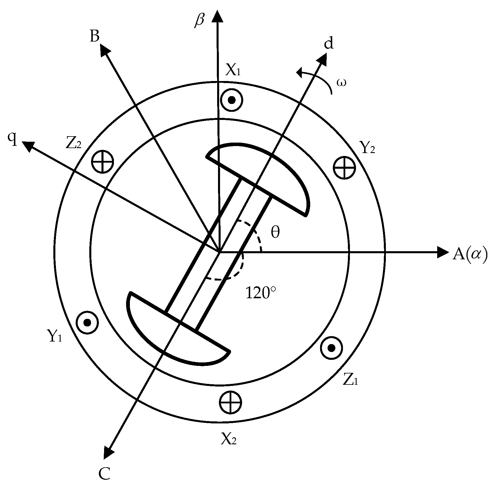
2. Physical and Mathematical Model of a PMSM

It is assumed that the stator winding of the PMSM is Y-connected, the windings of the three phases are symmetrically distributed, the axes are 120° apart from each other, and the variation in other parameters in the motor are neglected (resistance and inductance of the windings, etc.). The physical model is shown in Figure 1. The stator windings X₁X₂, Y₁Y₂, and Z₁Z₂ are symmetrically installed in a circular space, with X₁, Y₁, and Z₁ being the first ends of each winding and X₂, Y₂, and Z₂ being the last ends. The first end outflow and the last end inflow are specified as the positive direction of the current. According to the right-hand screw rule, the direction of the magnetic field generated by each winding is specified as the positive direction of the axis of the winding. Then, using these three directions as the reference axes of the spatial coordinate axes, a three-phase stationary coordinate system named $A-B-C$ is established. The counterclockwise direction is specified as the positive direction of the angle and angular velocity. In Figure 1, the two-phase stationary coordinate system $\alpha -\beta$ is used to fix the $\alpha$-axis and keep it stationary on the axis of the stator A-phase winding, while the $\beta$-axis is 90° ahead compared to the $\alpha$-axis. The two-phase rotating coordinate system $d-q$ consists of the orthogonal $d$-axis and $q$-axis. The direction of the $d$-axis is the direction of the flux linkage of the permanent magnet, and the angle between the $d$-axis and the $A$-axis is $\theta$. The coordinate transformation from $A-B-C$ to $\alpha -\beta$ is a Park transformation, and the transformation from $\alpha -\beta$ to $d-q$ is a Clarke transformation. The algorithm proposed in this paper is based on the mathematical model in the $\alpha -\beta$ coordinate system.

In the $\alpha -\beta$ coordinate system, the current equation of the state for a surface-mounted three-phase PMSM is expressed as

$$\left\{\begin{array}{l}\frac{d{i}_{\alpha }}{dt}=-\frac{R_s}{L_s}{i}_{\alpha }+\frac{1}{L_s}{u}_{\alpha }-\frac{1}{L_s}{e}_{\alpha }\\ \frac{d{i}_{\beta }}{dt}=-\frac{R_s}{L_s}{i}_{\beta }+\frac{1}{L_s}{u}_{\beta }-\frac{1}{L_s}{e}_{\beta }\end{array}\right.$$

(1)

where $R_s$ is the resistance of the stator; $u_{\alpha }$, $u_{\beta }$, $i_{\alpha }$, and $i_{\beta }$ are the voltage and current of the stator in the $\alpha -\beta$ coordinate system, respectively; and $e_{\alpha }$ and $e_{\beta }$ are the extended back-EMF, which is expressed using the following relation:

$$\left\{\begin{array}{l}{e}_{\alpha }=-{\psi }_f{\omega }_e\sin {\theta }_e\\ e_{\beta }={\psi }_f{\omega }_e\cos {\theta }_e\end{array}\right.$$

(2)

where ${\omega }_e$ and ${\theta }_e$ are the electrical angular velocity and the electrical angle of the rotor, respectively, and ${\psi }_f$ is the flux linkage of the permanent magnet.

In addition, the differential equation of Equation (2) is satisfied as follows:

$$\left\{\begin{array}{l}\frac{d{e}_{\alpha }}{dt}={\omega }_{\mathrm{e}}\left(-{\psi }_{\mathrm{f}}{\omega }_{\mathrm{e}}\cos {\theta }_{\mathrm{e}}\right)=-{\omega }_{\mathrm{e}}{e}_{\beta }\\ \frac{d{e}_{\beta }}{dt}={\omega }_{\mathrm{e}}\left(-{\psi }_{\mathrm{f}}{\omega }_{\mathrm{e}}\sin {\theta }_{\mathrm{e}}\right)={\omega }_{\mathrm{e}}{e}_{\alpha }\end{array}\right.$$

(3)

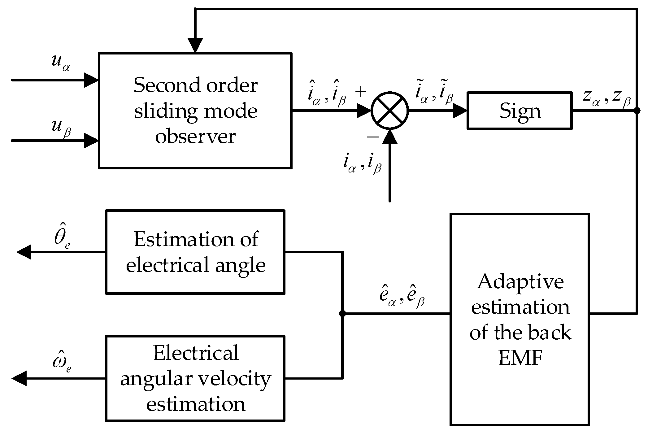
3. Second-Order Adaptive Sliding-Mode Observer Algorithm

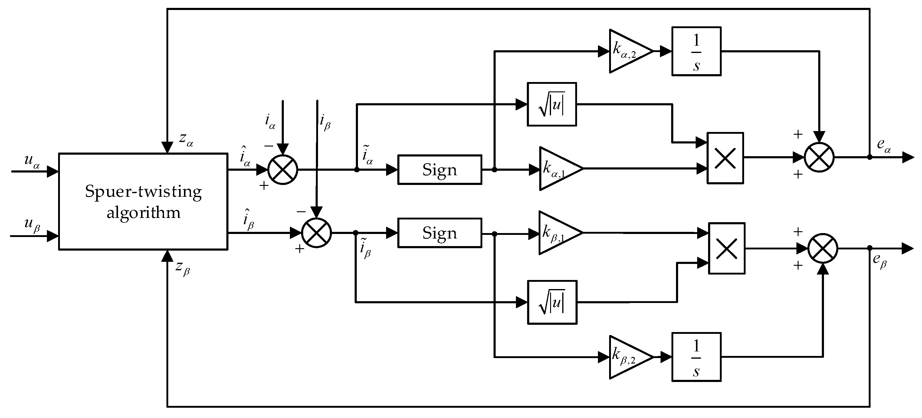
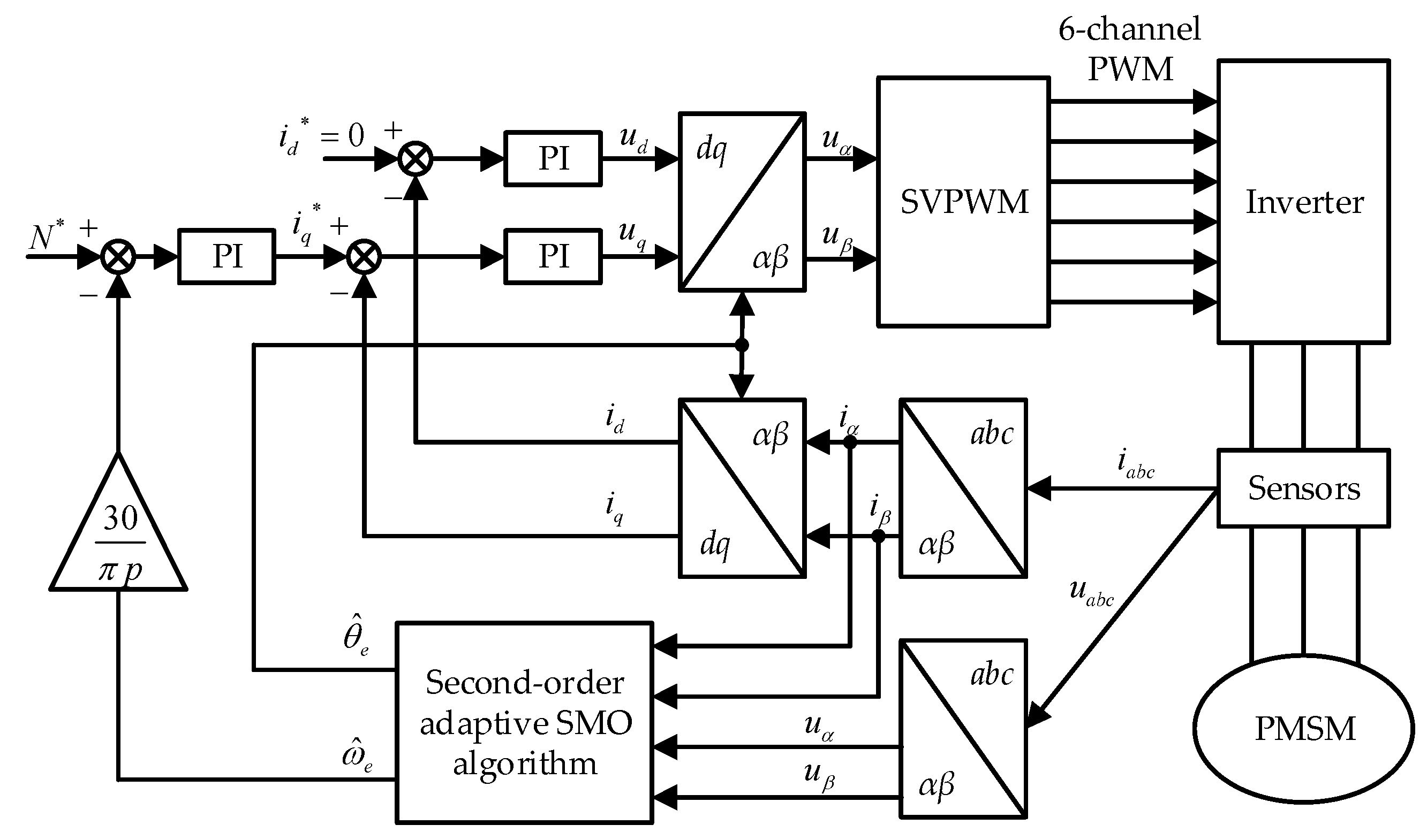
3.1. Design of Second-Order SMO

The super-twisting algorithm is expressed as [30]

$$\left\{\begin{array}{l}{\dot{x}}_1=-k_1{\left|x_1\right|}^{\frac{1}{2}}sign\left(x_1\right)+x_2+{\rho }_1\\ {\dot{x}}_2=-k_{2}sign\left(x_1\right)+{\rho }_2\end{array}\right.$$

(4)

where $k_i$ is the sliding-mode gain, $x_i$ is the state variable of the system, and ${\rho }_i$ is the disturbance term of the system.

The super-twisting algorithm transfers the discontinuous high-frequency switching term $k_{i}sign\left(x_i\right)$ in traditional sliding-mode control from $x_i$ to ${\dot{x}}_i$; that is, $k_{i}sign\left(x_i\right)$ no longer directly affects and controls $x_i$ but appears in the control law of the super-twisting second-order sliding-mode control in the form of time integration, thereby obtaining continuous control signals.

According to Equation (2), it is seen that the magnitude of the extended back-EMF is related to the angular velocity (${\omega }_{\mathrm{e}}$), the angle (${\theta }_{\mathrm{e}}$), and the flux linkage (${\psi }_{\mathrm{f}}$), where ${\psi }_{\mathrm{f}}$ is a fixed value; therefore, in order to obtain the velocity and position information of the rotor, the extended back-EMF should be obtained first. According to Equation (1), the sliding-mode observer is designed as follows:

$$\left\{\begin{array}{l}\frac{d{\widehat{i}}_{\alpha }}{dt}=-\frac{R_s}{L_s}{\widehat{i}}_{\alpha }+\frac{1}{L_s}{u}_{\alpha }-\frac{1}{L_s}{z}_{\alpha }\\ \frac{d{\widehat{i}}_{\beta }}{dt}=-\frac{R_s}{L_s}{\widehat{i}}_{\beta }+\frac{1}{L_s}{u}_{\beta }-\frac{1}{L_s}{z}_{\beta }\end{array}\right.$$

(5)

where $z_{\alpha }$ and $z_{\beta }$ are the inputs of the sliding-mode observer and ${\widehat{i}}_{\alpha }$ and ${\widehat{i}}_{\beta }$ are the observed values of the current.

Subtract Equation (1) from Equation (5), the error equation for the stator current is obtained:

$$\left\{\begin{array}{l}\frac{d{\tilde{i}}_{\alpha }}{dt}=-\frac{R_s}{L_s}{\tilde{i}}_{\alpha }-\frac{1}{L_s}\left(z_{\alpha }-e_{\alpha }\right)\\ \frac{d{\tilde{i}}_{\beta }}{dt}=-\frac{R_s}{L_s}{\tilde{i}}_{\beta }-\frac{1}{L_s}\left(z_{\beta }-e_{\beta }\right)\end{array}\right.$$

(6)

where ${\tilde{i}}_{\alpha }={\widehat{i}}_{\alpha }-i_{\alpha }$ and ${\tilde{i}}_{\beta }={\widehat{i}}_{\beta }-i_{\beta }$ are the observed error of the stator current. Taking the main sliding-mode surface, $s={\left[{\tilde{i}}_{\alpha }{\tilde{i}}_{\beta }\right]}^T$.

According to the constant reaching law, the sliding-mode control law is designed as:

$$\left\{\begin{array}{l}{z}_{\alpha }=k_{\alpha ,1}{\left|{\tilde{i}}_{\alpha }\right|}^{\frac{1}{2}}sign\left({\tilde{i}}_{\alpha }\right)+{\eta }_{\alpha ,1}\\ {\dot{\eta }}_{\alpha ,1}=k_{\alpha ,2}sign\left({\tilde{i}}_{\alpha }\right)\\ z_{\beta }=k_{\beta ,1}{\left|{\tilde{i}}_{\beta }\right|}^{\frac{1}{2}}sign\left({\tilde{i}}_{\beta }\right)+{\eta }_{\beta ,1}\\ {\dot{\eta }}_{\beta ,1}=k_{\beta ,2}sign\left({\tilde{i}}_{\beta }\right)\end{array}\right.$$

(7)

where $k_{i,j}$ is the sliding-mode observer gain; ${\dot{\eta }}_{\alpha ,1}$ and ${\dot{\eta }}_{\beta ,1}$ are the observed values of the auxiliary sliding-mode surface; and $sign\left({\tilde{i}}_{\alpha }\right)$ and $sign\left({\tilde{i}}_{\beta }\right)$ are symbolic functions that are satisfied as follows:

$$\left\{\begin{array}{l}sign\left({\tilde{i}}_{\alpha }\right)=\left\{\begin{array}{l}1, {\tilde{i}}_{\alpha }\ge 0\\ -1, {\tilde{i}}_{\alpha }<0\end{array}\right.\\ sign\left({\tilde{i}}_{\beta }\right)=\left\{\begin{array}{l}1, {\tilde{i}}_{\beta }\ge 0\\ -1, {\tilde{i}}_{\beta }<0\end{array}\right.\end{array}\right.$$

(8)

Taking Equation (7) into Equation (6), a new error equation for the stator current is obtained:

$$\left\{\begin{array}{l}\frac{d{\tilde{i}}_{\alpha }}{dt}=-{\lambda }_{\alpha ,1}{\left|{\tilde{i}}_{\alpha }\right|}^{\frac{1}{2}}sign\left({\tilde{i}}_{\alpha }\right)+{\eta }_{\alpha }+{\rho }_{\alpha }\\ {\dot{\eta }}_{\alpha }=-{\lambda }_{\alpha ,2}sign\left({\tilde{i}}_{\alpha }\right),{\rho }_{\alpha }=-\frac{R_s}{L_s}{\tilde{i}}_{\alpha }+\frac{1}{L_s}{e}_{\alpha }\\ \frac{d{\tilde{i}}_{\beta }}{dt}=-{\lambda }_{\beta ,1}{\left|{\tilde{i}}_{\beta }\right|}^{\frac{1}{2}}sign\left({\tilde{i}}_{\beta }\right)+{\eta }_{\beta }+{\rho }_{\beta }\\ {\dot{\eta }}_{\beta }=-{\lambda }_{\beta ,2}sign\left({\tilde{i}}_{\beta }\right),{\rho }_{\beta }=-\frac{R_s}{L_s}{\tilde{i}}_{\beta }+\frac{1}{L_s}{e}_{\beta }\end{array}\right.$$

(9)

where ${\lambda }_{\alpha ,1}=\frac{k_{\alpha ,1}}{L_s}$, ${\lambda }_{\alpha ,2}=\frac{k_{\alpha ,2}}{L_s}$, ${\lambda }_{\beta ,1}=\frac{k_{\beta ,1}}{L_s}$, and ${\lambda }_{\beta ,2}=\frac{k_{\beta ,2}}{L_s}$. Comparing Equations (4) and (9), ${\rho }_{\alpha }$ and ${\rho }_{\beta }$ are the disturbance terms of the system. For ${\delta }_1,{\delta }_2\ge 0$, ${\rho }_{\alpha }$ and ${\rho }_{\beta }$ are satisfied according to the following relation:

$$\left\{\begin{array}{l}\left|{\rho }_{\alpha }\right|\le {\delta }_1{\left|{\tilde{i}}_{\alpha }\right|}^{\frac{1}{2}}\\ \left|{\rho }_{\beta }\right|\le {\delta }_2{\left|{\tilde{i}}_{\beta }\right|}^{\frac{1}{2}}\end{array}\right.$$

(10)

When the system state reaches the sliding-mode surface, $s=0,\dot{s}=0$, i.e., ${\tilde{i}}_{\alpha }={\tilde{i}}_{\beta }=0$ and $\frac{d{\tilde{i}}_{\alpha }}{dt}=\frac{d{\tilde{i}}_{\beta }}{dt}=0$. Taking them into Equation (6), at this time, $z_{\alpha }$ and $z_{\beta }$ are equivalent to the extended back-EMF ($e_{\alpha }$ and $e_{\beta }$) and are expressed as

$$\left\{\begin{array}{l}{e}_{\alpha }=z_{\alpha }=k_{\alpha ,1}{\left|{\tilde{i}}_{\alpha }\right|}^{\frac{1}{2}}sign\left({\tilde{i}}_{\alpha }\right)+{\displaystyle \int k_{\alpha ,2}sign\left({\tilde{i}}_{\alpha }\right)}\\ e_{\beta }=z_{\beta }=k_{\beta ,1}{\left|{\tilde{i}}_{\beta }\right|}^{\frac{1}{2}}sign\left({\tilde{i}}_{\beta }\right)+{\displaystyle \int k_{\beta ,2}sign\left({\tilde{i}}_{\beta }\right)}\end{array}\right.$$

(11)

A structural block diagram of the second-order sliding-mode observer algorithm is shown in Figure 2. First, according to Equation (5), the estimated values of the stator current (${\widehat{i}}_{\alpha }$ and ${\widehat{i}}_{\beta }$) are obtained using the voltage of the stator ($u_{\alpha }$ and $u_{\beta }$) and the feedback values ($z_{\alpha }$ and $z_{\beta }$). Then, the difference is subtracted from the actual current values ($i_{\alpha }$ and $i_{\beta }$) collected by the circuit to obtain the observed error of the stator current (${\tilde{i}}_{\alpha }$ and ${\tilde{i}}_{\beta }$). Finally, according to Equation (11), the observed error of the stator current is further processed to obtain $z_{\alpha }$ and $z_{\beta }$ and the extended back-EMF ($e_{\alpha }$ and $e_{\beta }$). Then, $z_{\alpha }$ and $z_{\beta }$ are fed back to the first step of the algorithm to realize closed-loop control.

The stability of the second-order SMO plays an important role in the application, so the Lyapunov function is adopted to verify the stability and the area of algorithm. The Lyapunov function is set as

$$\left\{\begin{array}{l}{V}_0=V_{\alpha }\left({\tilde{i}}_{\alpha }\right)+V_{\beta }\left({\tilde{i}}_{\beta }\right)\\ =2{\lambda }_{\alpha ,2}\left|{\tilde{i}}_{\alpha }\right|+\frac{1}{2}{\eta }_{\alpha }{}^2+\frac{1}{2}{\left({\lambda }_{\alpha ,1}{\left|{\tilde{i}}_{\alpha }\right|}^{\frac{1}{2}}sign\left({\tilde{i}}_{\alpha }\right)-{\eta }_{\alpha }\right)}^2\\ +2{\lambda }_{\beta ,2}\left|{\tilde{i}}_{\beta }\right|+\frac{1}{2}{\eta }_{\beta }{}^2+\frac{1}{2}{\left({\lambda }_{\beta ,1}{\left|{\tilde{i}}_{\beta }\right|}^{\frac{1}{2}}sign\left({\tilde{i}}_{\beta }\right)-{\eta }_{\beta }\right)}^2\\ ={\gamma }_{\alpha }{}^T{P}_{\alpha }{\gamma }_{\alpha }+{\gamma }_{\beta }{}^T{P}_{\beta }{\gamma }_{\beta }\end{array}\right.$$

(12)

where

$$\left[{\gamma }_{\alpha }{\gamma }_{\beta }\right]=\left[\begin{array}{l}{\left|{\tilde{i}}_{\alpha }\right|}^{\frac{1}{2}}sign\left({\tilde{i}}_{\alpha }\right){\left|{\tilde{i}}_{\beta }\right|}^{\frac{1}{2}}sign\left({\tilde{i}}_{\beta }\right)\\ \hspace{1em}\hspace{1em} {\eta }_{\alpha }\hspace{1em}\hspace{1em}\hspace{1em}\hspace{1em}{\eta }_{\beta }\end{array}\right]$$

(13)

$$P_{\alpha }=\frac{1}{2}\left[\begin{array}{l}4{\lambda }_{\alpha ,2}+{\lambda }_{\alpha ,1}{}^2-{\lambda }_{\alpha ,1}\\ \hspace{1em}-{\lambda }_{\alpha ,1}\hspace{1em}\hspace{1em}\hspace{1em}2\end{array}\right]$$

(14)

$$P_{\beta }=\frac{1}{2}\left[\begin{array}{l}4{\lambda }_{\beta ,2}+{\lambda }_{\beta ,1}{}^2-{\lambda }_{\beta ,1}\\ \hspace{1em}-{\lambda }_{\beta ,1}\hspace{1em}\hspace{1em}\hspace{1em}2\end{array}\right]$$

(15)

The derivative of $V_0$ is given by

$${\dot{V}}_0=-\frac{1}{{\left|{\tilde{i}}_{\alpha }\right|}^{\frac{1}{2}}}{\gamma }_{\alpha }{}^T{Q}_{\alpha }{\gamma }_{\alpha }-\frac{1}{{\left|{\tilde{i}}_{\beta }\right|}^{\frac{1}{2}}}{\gamma }_{\beta }{}^T{Q}_{\beta }{\gamma }_{\beta }$$

(16)

where

$$Q_{\alpha }=\frac{{\lambda }_{\alpha ,1}}{2}\left[\begin{array}{l}2{\lambda }_{\alpha ,2}+{\lambda }_{\alpha ,1}{}^2-{\lambda }_{\alpha ,1}\\ \hspace{1em}-{\lambda }_{\alpha ,1}\hspace{1em}\hspace{1em}\hspace{1em}1\end{array}\right]$$

(17)

$$Q_{\beta }=\frac{{\lambda }_{\beta ,1}}{2}\left[\begin{array}{l}2{\lambda }_{\beta ,2}+{\lambda }_{\beta ,1}{}^2-{\lambda }_{\beta ,1}\\ \hspace{1em}-{\lambda }_{\beta ,1}\hspace{1em}\hspace{1em}\hspace{1em}1\end{array}\right]$$

(18)

In Equation (12), $V_0$ is continuous, but it is not differentiable when ${\tilde{i}}_{\alpha }={\tilde{i}}_{\beta }=0$. When ${\lambda }_{\alpha ,1},{\lambda }_{\alpha ,2},{\lambda }_{\beta ,1},{\lambda }_{\beta ,2}>0$, $V_0$ is positive and definite and ${\dot{V}}_0$ is negative and definite. In this case, reference [31] amply demonstrated that a control system tends to stabilize if the disturbance term is globally bounded, i.e., Equation (10) holds, and the sliding-mode gain satisfies the following relation (19):

$$\left\{\begin{array}{l}{\lambda }_{\alpha ,1}>2{\delta }_1\\ {\lambda }_{\alpha ,2}>{\lambda }_{\alpha ,1}\frac{5{\delta }_1{\lambda }_{\alpha ,1}+4{\delta }_1{}^2}{2\left({\lambda }_{\alpha ,1}-2{\delta }_1\right)}\\ {\lambda }_{\beta ,1}>2{\delta }_2\\ {\lambda }_{\beta ,2}>{\lambda }_{\beta ,1}\frac{5{\delta }_2{\lambda }_{\beta ,1}+4{\delta }_2{}^2}{2\left({\lambda }_{\beta ,1}-2{\delta }_2\right)}\end{array}\right.$$

(19)

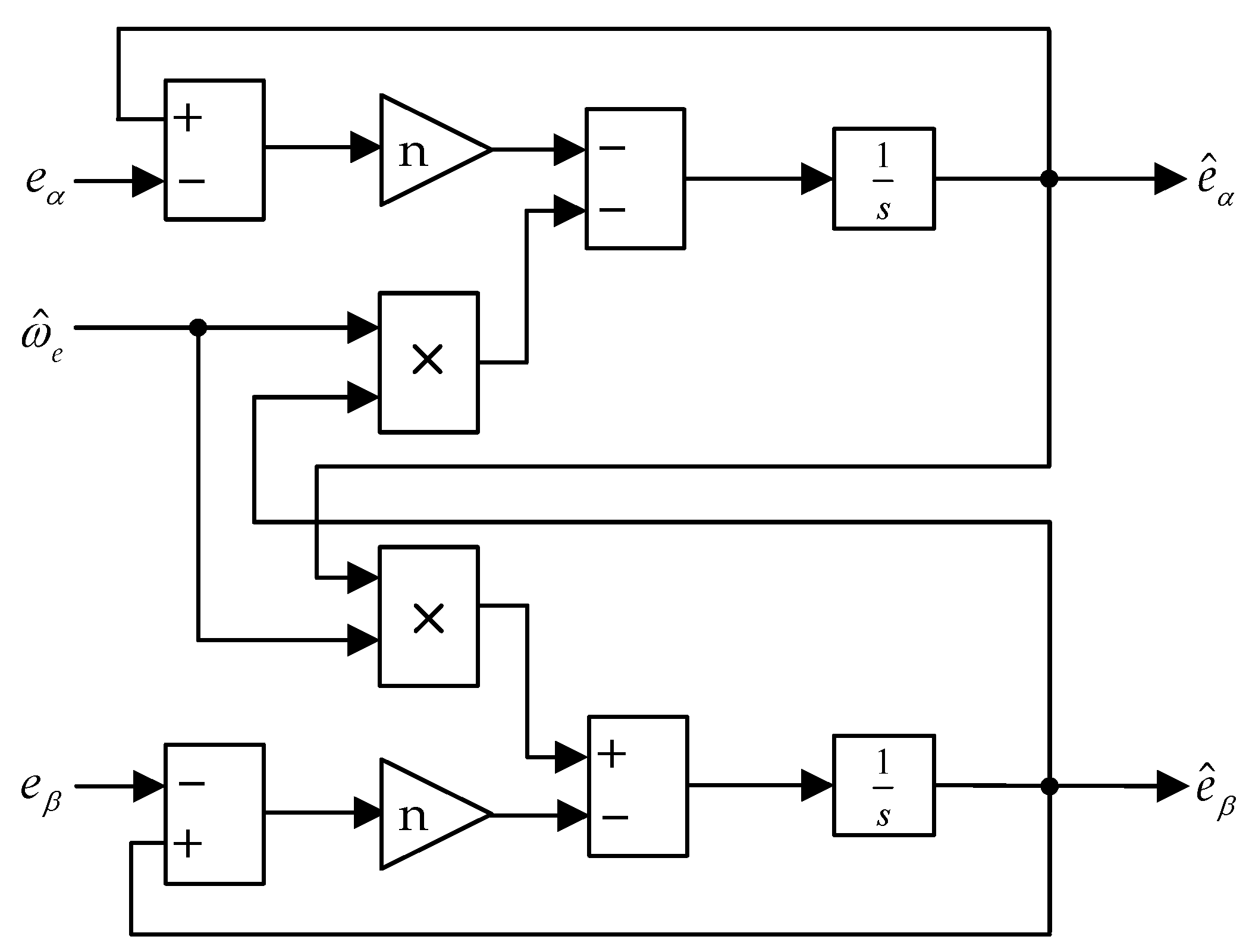
3.2. Adaptive Estimation of the Back-EMF

In the SMO algorithm, the jitter caused by the high-frequency harmonics is serious. In order to improve the estimation accuracy of the rotor position, reduce the high-frequency harmonics in the back-EMF, and make the back-EMF estimation smoother, a link of the adaptive estimation of the back-EMF is introduced. According to Equation (3), the adaptive law of the back-EMF is designed as

$$\left\{\begin{array}{l}\frac{d{\widehat{e}}_{\alpha }}{dt}=-{\widehat{\omega }}_e{\widehat{e}}_{\beta }-n{\tilde{e}}_{\alpha }\\ \frac{d{\widehat{e}}_{\beta }}{dt}={\widehat{\omega }}_e{\widehat{e}}_{\alpha }-n{\tilde{e}}_{\beta }\\ \frac{d{\widehat{\omega }}_e}{dt}={\tilde{e}}_{\alpha }{\widehat{e}}_{\beta }-{\widehat{e}}_{\alpha }{\tilde{e}}_{\beta }\end{array}\right.$$

(20)

where ${\widehat{\omega }}_e$ is the estimated value of the electrical angular velocity; ${\widehat{e}}_{\alpha }$ and ${\widehat{e}}_{\beta }$ are the estimated values of the adaptive link; $n$ is a positive constant; ${\tilde{e}}_{\alpha }={\widehat{e}}_{\alpha }-e_{\alpha }$; and ${\tilde{e}}_{\beta }={\widehat{e}}_{\beta }-e_{\beta }$.

Since the mechanical time constant is much longer than the electrical time constant during the rotation of the motor, the magnitude of the motor velocity can be considered to be constant during an estimated cycle, i.e., $\frac{d{\omega }_e}{dt}=0$. Accordingly, subtract Equation (3) from Equation (20) to obtain:

$$\left\{\begin{array}{l}\frac{d{\tilde{e}}_{\alpha }}{dt}=-{\widehat{\omega }}_e{\widehat{e}}_{\beta }-n{\tilde{e}}_{\alpha }+{\omega }_e{e}_{\beta }\\ \frac{d{\tilde{e}}_{\beta }}{dt}={\widehat{\omega }}_e{\widehat{e}}_{\alpha }-n{\tilde{e}}_{\beta }-{\omega }_e{e}_{\alpha }\\ \frac{d{\tilde{\omega }}_e}{dt}={\tilde{e}}_{\alpha }{\widehat{e}}_{\beta }-{\widehat{e}}_{\alpha }{\tilde{e}}_{\beta }\end{array}\right.$$

(21)

It is necessary to construct the Lyapunov function to verify the stability of the link of adaptive estimation. The Lyapunov function is constructed as

$$V_1=\frac{1}{2}{\tilde{e}}_{\alpha }{}^2+\frac{1}{2}{\tilde{e}}_{\beta }{}^2+\frac{1}{2}{\tilde{\omega }}_e{}^2$$

(22)

The derivative of $V_1$ is calculated as follows:

$$\begin{array}{ll}{\dot{V}}_1& ={\tilde{e}}_{\alpha }{\dot{\tilde{e}}}_{\alpha }+{\tilde{e}}_{\beta }{\dot{\tilde{e}}}_{\beta }+{\tilde{\omega }}_e{\dot{\tilde{\omega }}}_e\\ & =-n\left({\tilde{e}}_{\alpha }{}^2+{\tilde{e}}_{\beta }{}^2\right)\le 0\end{array}$$

(23)

From Equations (22) and (23), a conclusion is reached. $V_1$ is positive and definite, and ${\dot{V}}_1$ is negative and definite, which is consistent with Lyapunov’s stability theorem, so the algorithm is stable. Figure 3 below shows a structural block diagram of the link of adaptive estimation.

3.3. Calculation of Rotor Velocity and Position

Since the link of adaptive estimation of the back-EMF is adopted in the algorithm and the low-pass filter is not used, the problem of the phase delay caused by the filter is avoided, so the additional compensation of the electric angular velocity is not necessary. The estimated value of the electric angle (${\widehat{\theta }}_e$) and the estimated value of the electric angular velocity (${\widehat{\omega }}_e$) are calculated according to Equation (2):

$$\left\{\begin{array}{l}{\widehat{\theta }}_e=\arctan \left(-\frac{{\widehat{e}}_{\alpha }}{{\widehat{e}}_{\beta }}\right)\\ {\widehat{\omega }}_e=\frac{\sqrt{{\widehat{e}}_{\alpha }{}^2+{\widehat{e}}_{\beta }{}^2}}{{\psi }_f}\end{array}\right.$$

(24)

The structure of the designed second-order adaptive sliding-mode observer algorithm is shown in Figure 4.

4. Experiment Verification and Results Analysis

Based on a test bench, the second-order adaptive SMO algorithm was integrated into the basic software of the PMSM control system, whose basic structure block diagram is shown in Figure 5. Since the current on the $d$-axis did not contribute to the increase in torque, it was possible to set the current on the $d$-axis to 0 and only control the current on the $q$-axis in order to make maximum use of the current, i.e., using a method with a reference value of 0 for the $i_d$($i_d{}^{*}$). The control system contained the closed-loop velocity and the closed-loop current, and the new algorithm was designed to observe the rotor velocity and angle in real time when the motor rotates. The observed velocity (${\widehat{\omega }}_e$) was converted to r/min and differed from the given velocity ($N^{*}$). The difference was calculated by the PI regulator of the closed-loop velocity as the reference current value ($i_q{}^{*}$) for the $q$-axis. Using the observed angle (${\widehat{\theta }}_e$), the sampled $i_a$, $i_b$, and $i_c$ were Clarke-transformed and Park-transformed to obtain $i_d$ and $i_q$. Then, $i_d$ and $i_q$ differed from the reference currents $i_d{}^{*}$ and $i_q{}^{*}$, respectively. The difference values were sent to the PI regulator to obtain $u_d$ and $u_q$. Finally, $u_{\alpha }$ and $u_{\beta }$ were input directly into the SVPWM module through the inverse Park transformation, and the six PWM signals for inverter control were generated to drive the motor. The main parameters of the PMSM are shown in

Table 1. Main parameters of PMSM.

Parameters	Values
Stator resistance (Rs/Ω)	3
Stator inductance (Ls/H)	0.01
Permanent magnet flux linkage (ψf/(Wb))	0.175
Moment of inertia (J/(kg·m^2))	0.001
Number of pole pairs	4
Rated power (Pn/kW)	1.2

.

The working conditions were $i_d{}^{*}=0$; DC-side voltage: $U_{dc}=311\mathrm{V}$; sliding-mode observer gain: $k_{\alpha ,1}=k_{\beta ,1}=600$ and $k_{\alpha ,2}=k_{\beta ,2}=10$; and the parameters in the adaptive law of the back-EMF: $n=5\times {10}^4$.

The working time of the model was 0.15 s. The initial velocity of the motor was set to 800 r/min. Then, the velocity increased abruptly from 800 r/min to 1000 r/min at 0.05 s. The load torque increased from 0 to 5 N·m at 0.10 s.

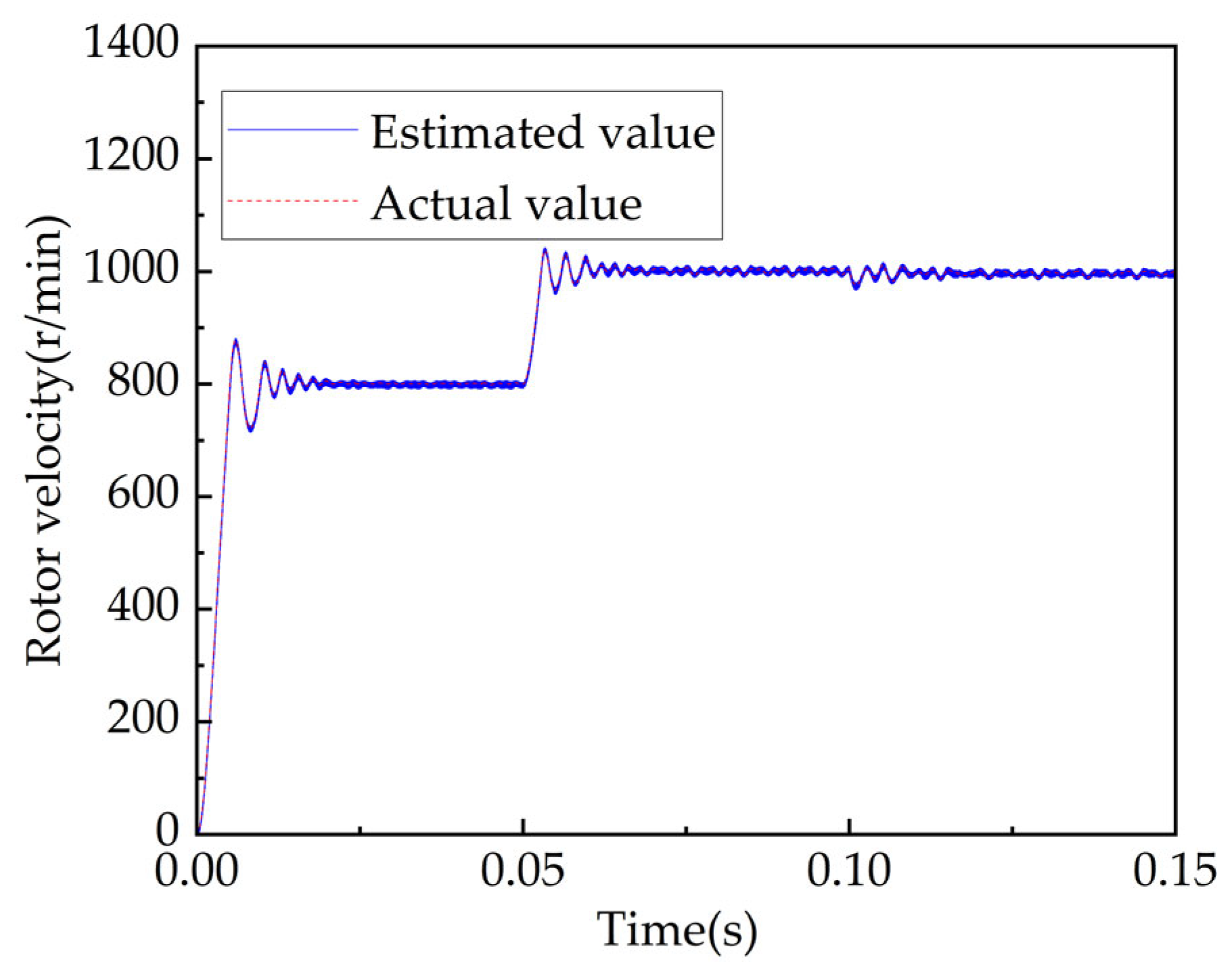
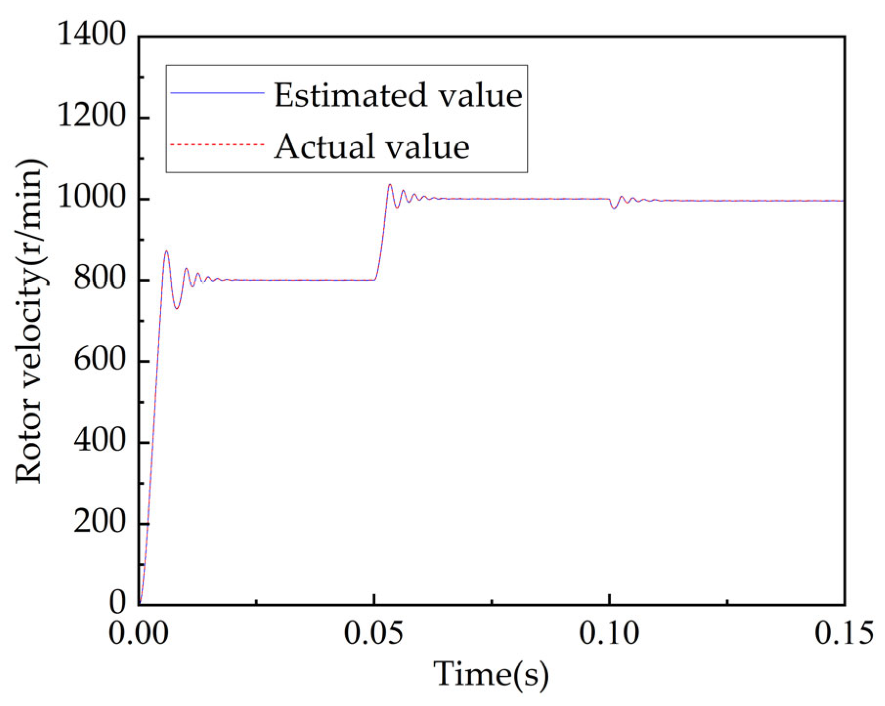
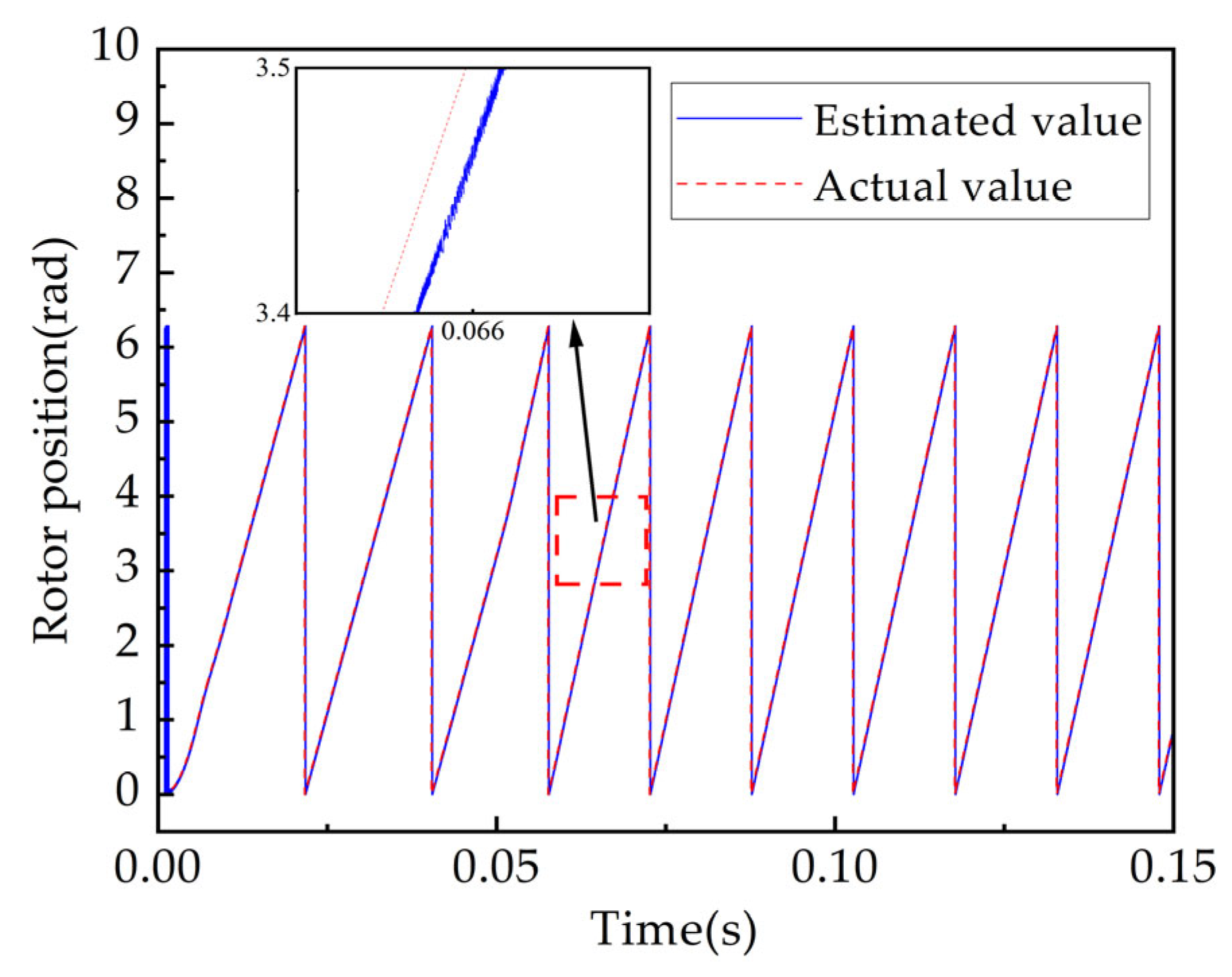
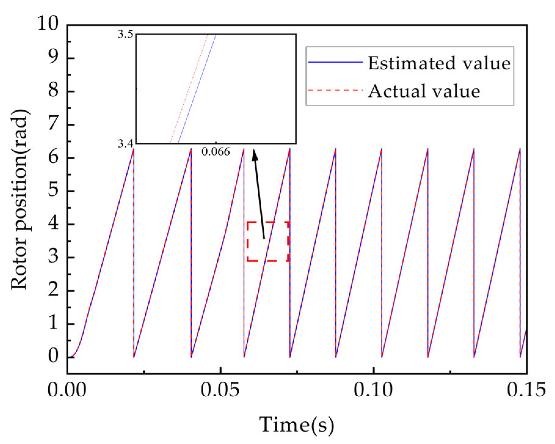
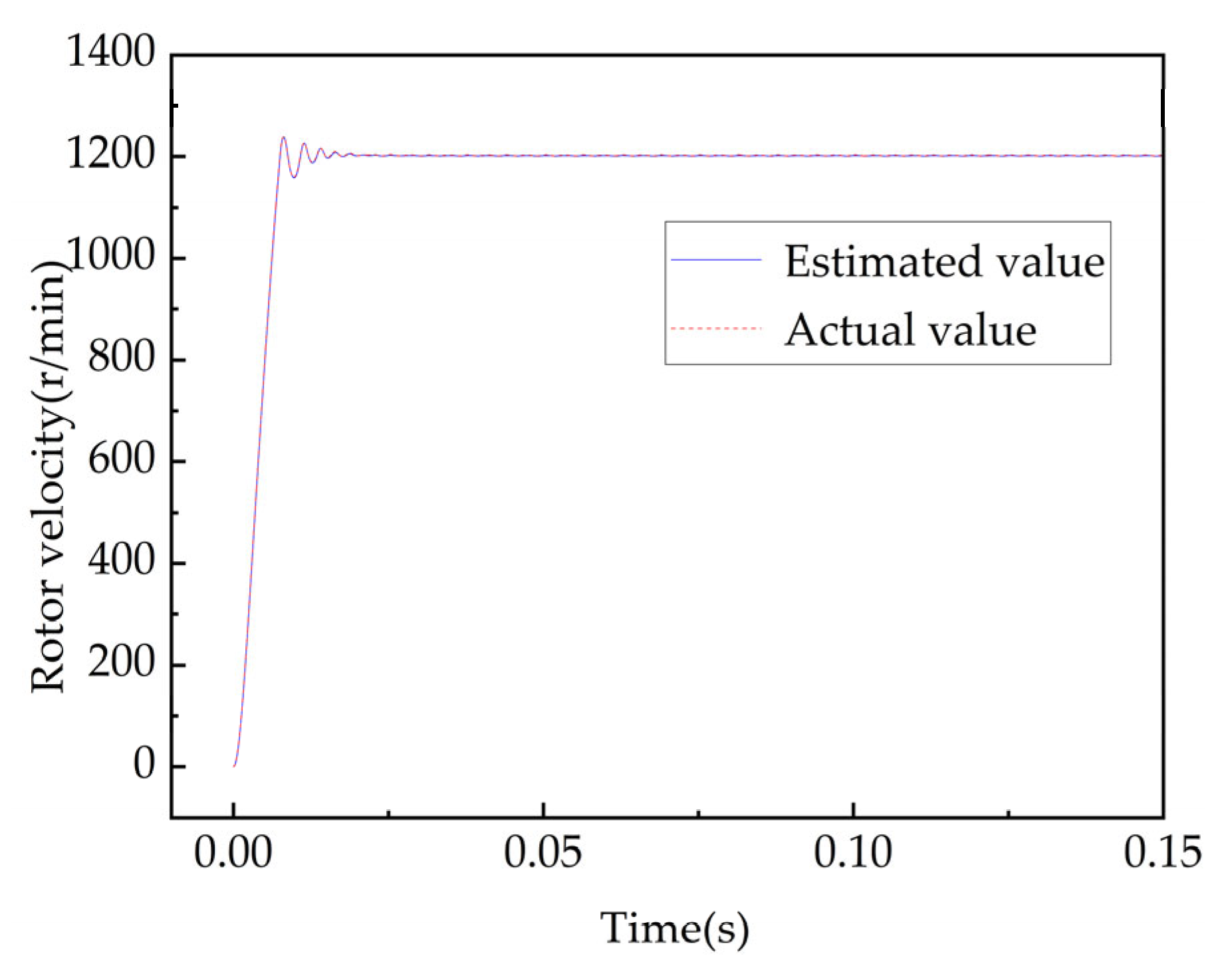
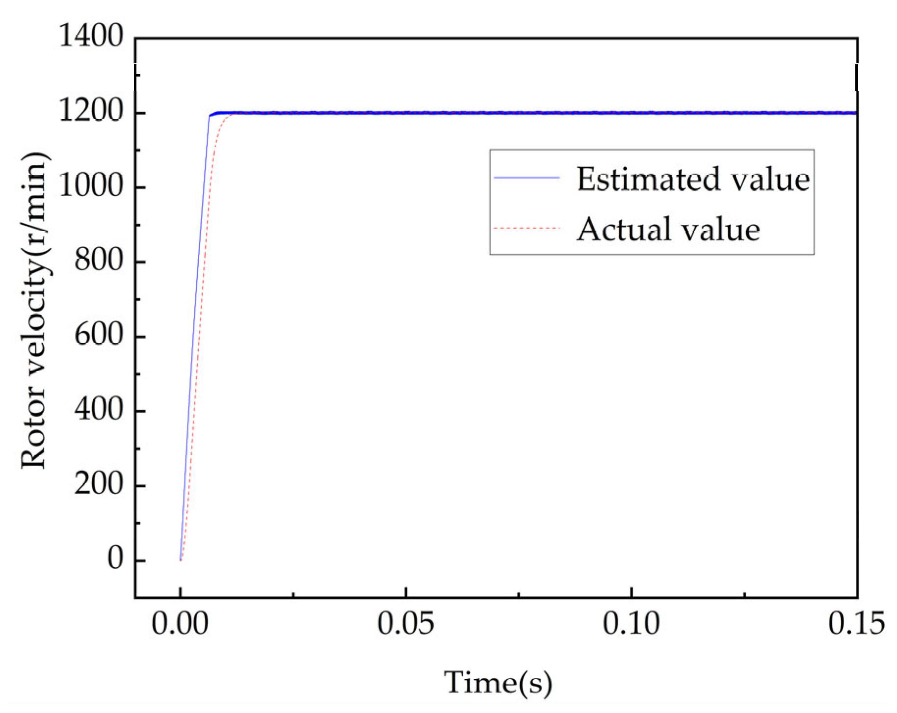
4.1. Analysis of Rotor Velocity and Rotor Position

Figure 6 and Figure 7 show the results of the rotor velocity and the estimated values for the traditional SMO algorithm and the second-order adaptive SMO algorithm in the given conditions. Figure 8 and Figure 9 show the results of the rotor position and the estimated values for the two algorithms for the given conditions.

From the results, it can be seen that both the traditional SMO algorithm and the second-order adaptive SMO algorithm were able to track the velocity and position of the system well. However, by comparing the characteristics in Figure 6 and Figure 7, it can be clearly seen that the estimated velocity curve of the traditional SMO algorithm was very jittery, while the estimated velocity curve of the second-order adaptive SMO algorithm was smooth, which indicates that the velocity estimation fluctuation of the algorithm was significantly reduced. Expanding Figure 8 and Figure 9 in the vicinity of 0.066 s also clearly showed that the estimated position curve of the traditional SMO algorithm had a lot of perturbations, while the estimated position curve of the second-order adaptive SMO algorithm was very smooth, which indicates that the fluctuation of the position estimate of the algorithm was also significantly reduced. Obviously, the tracking process of the second-order adaptive SMO algorithm is more stable.

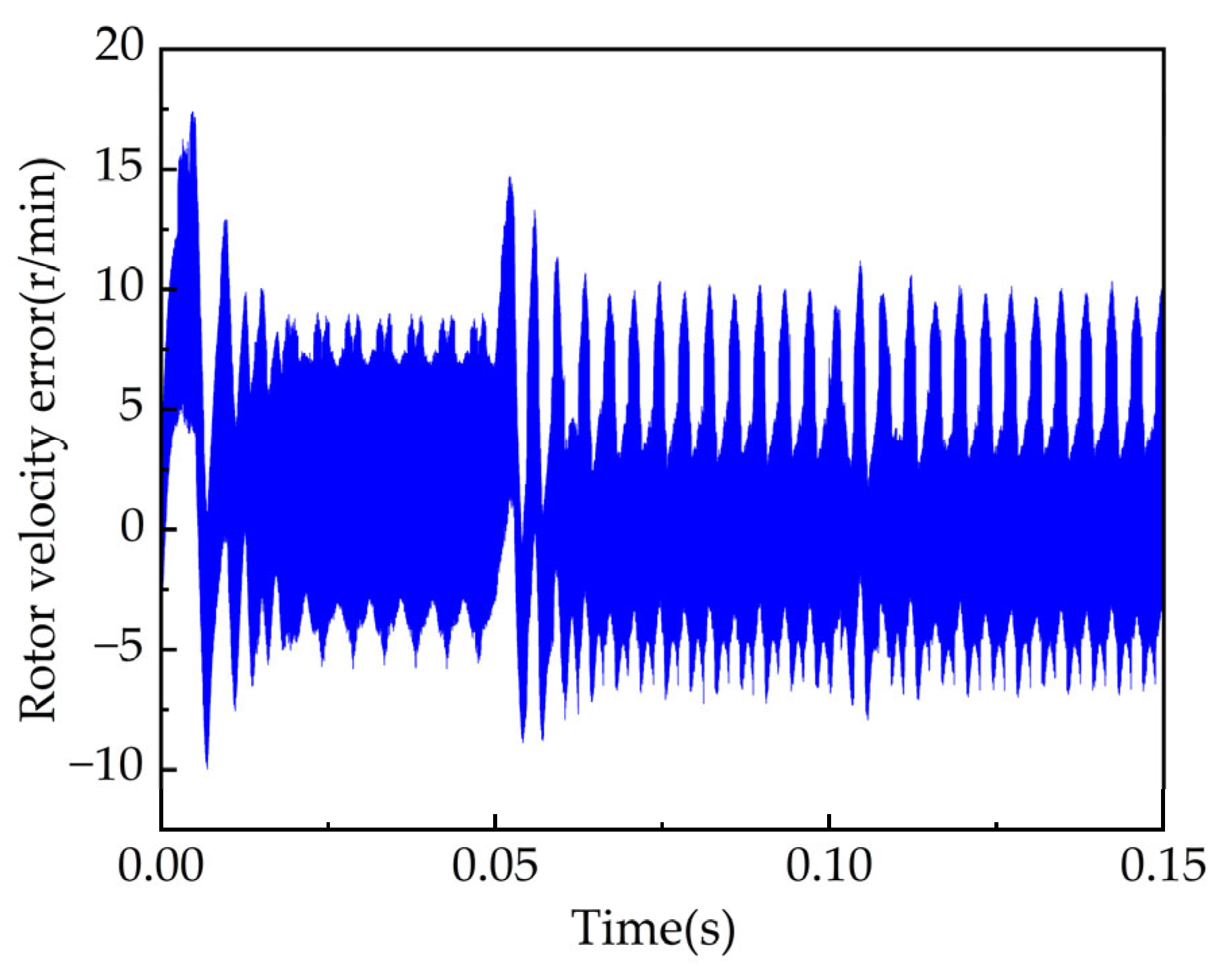
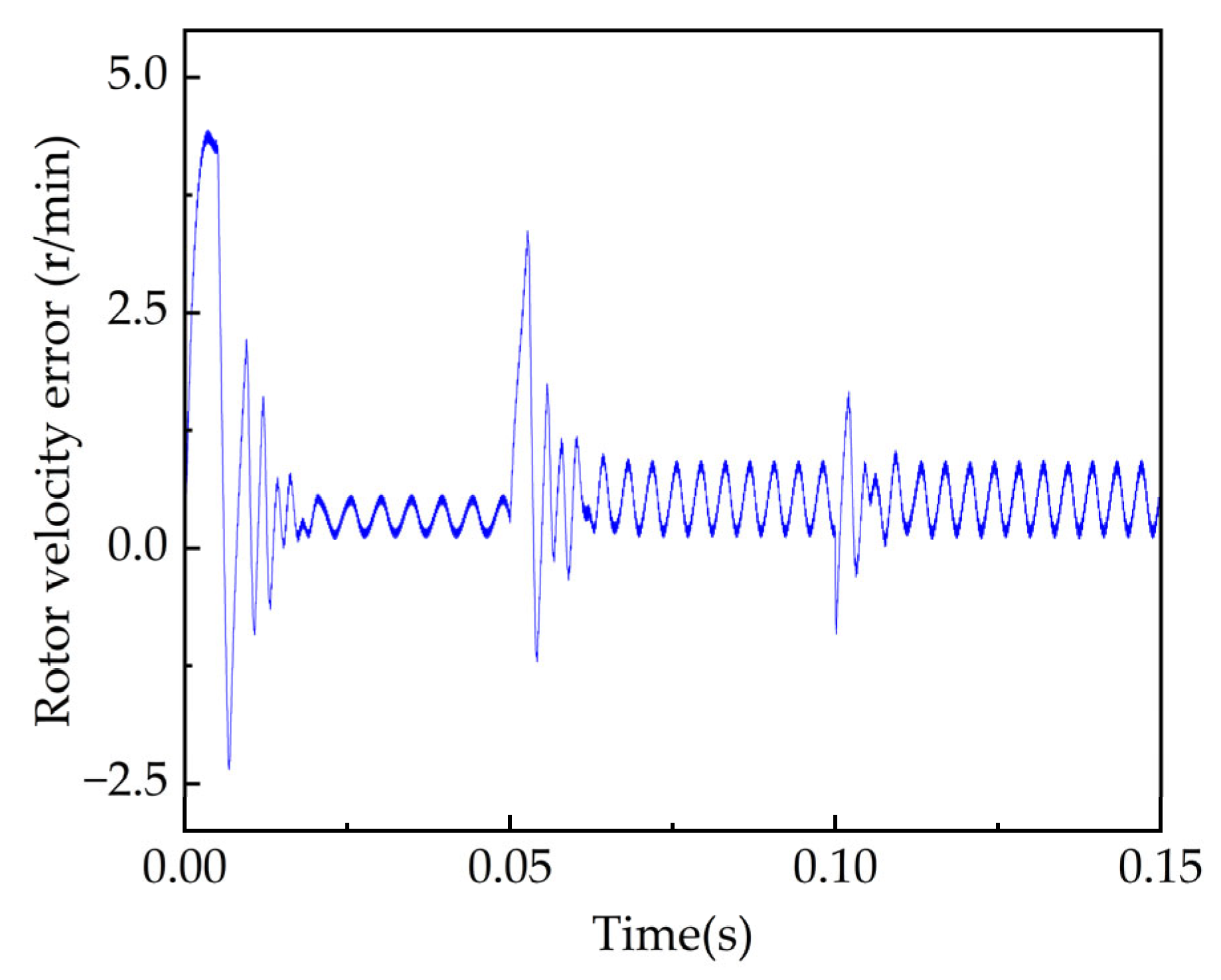
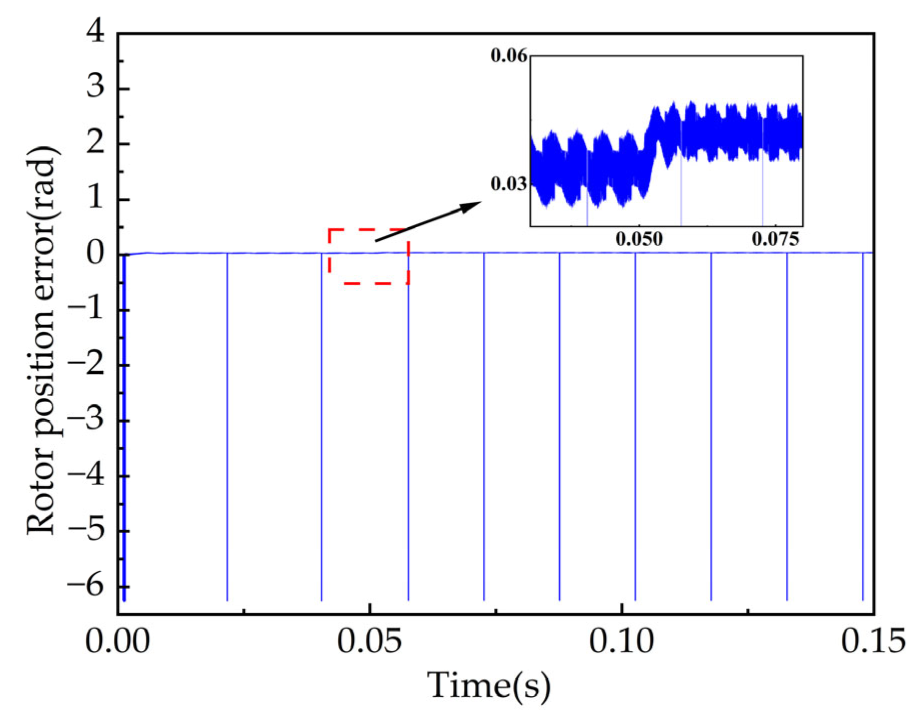
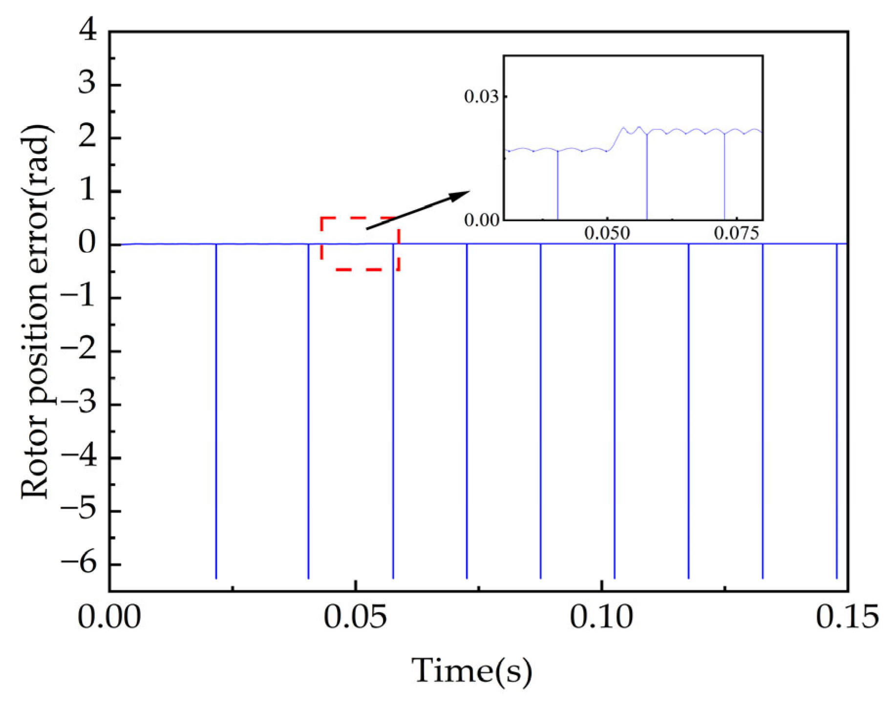
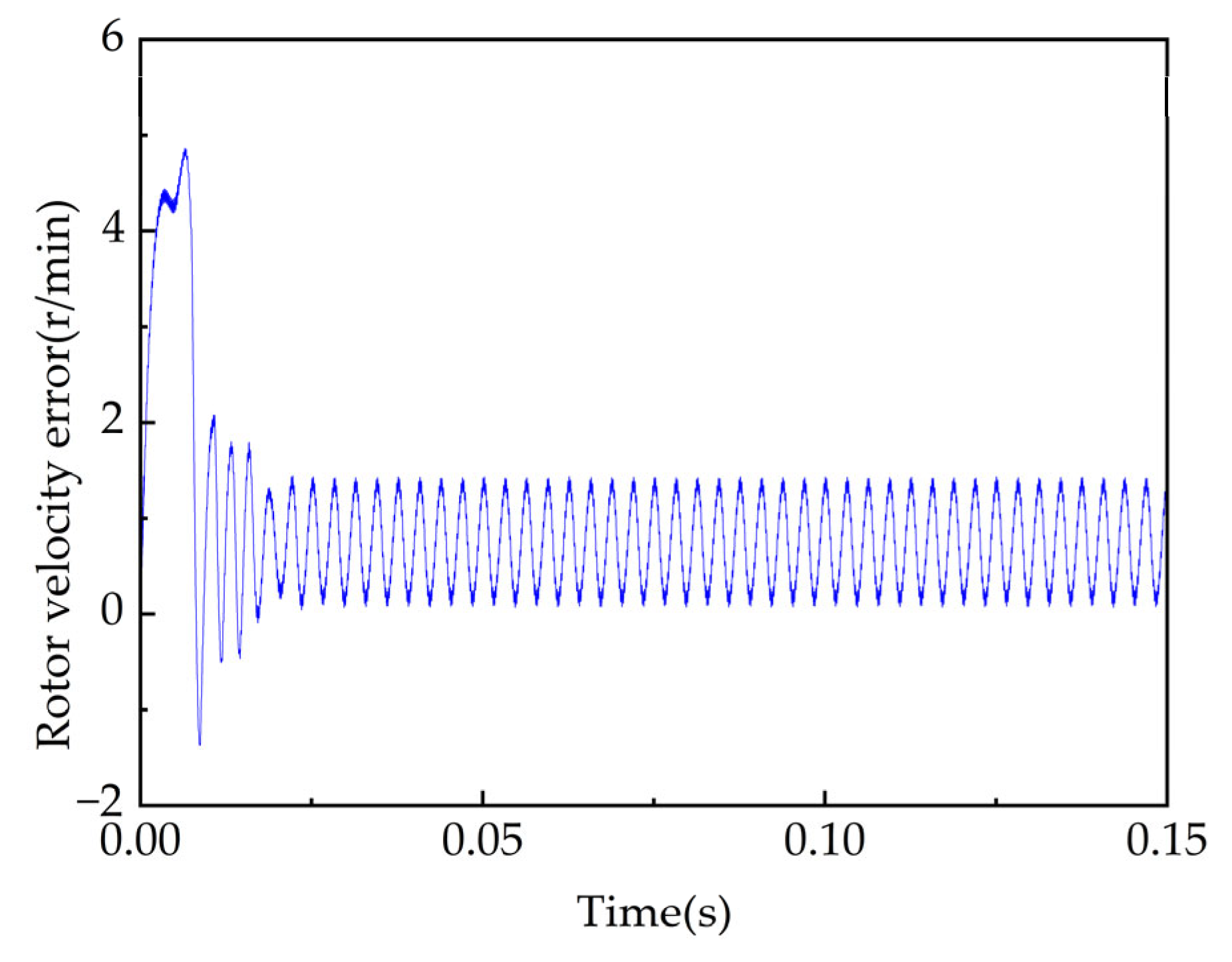
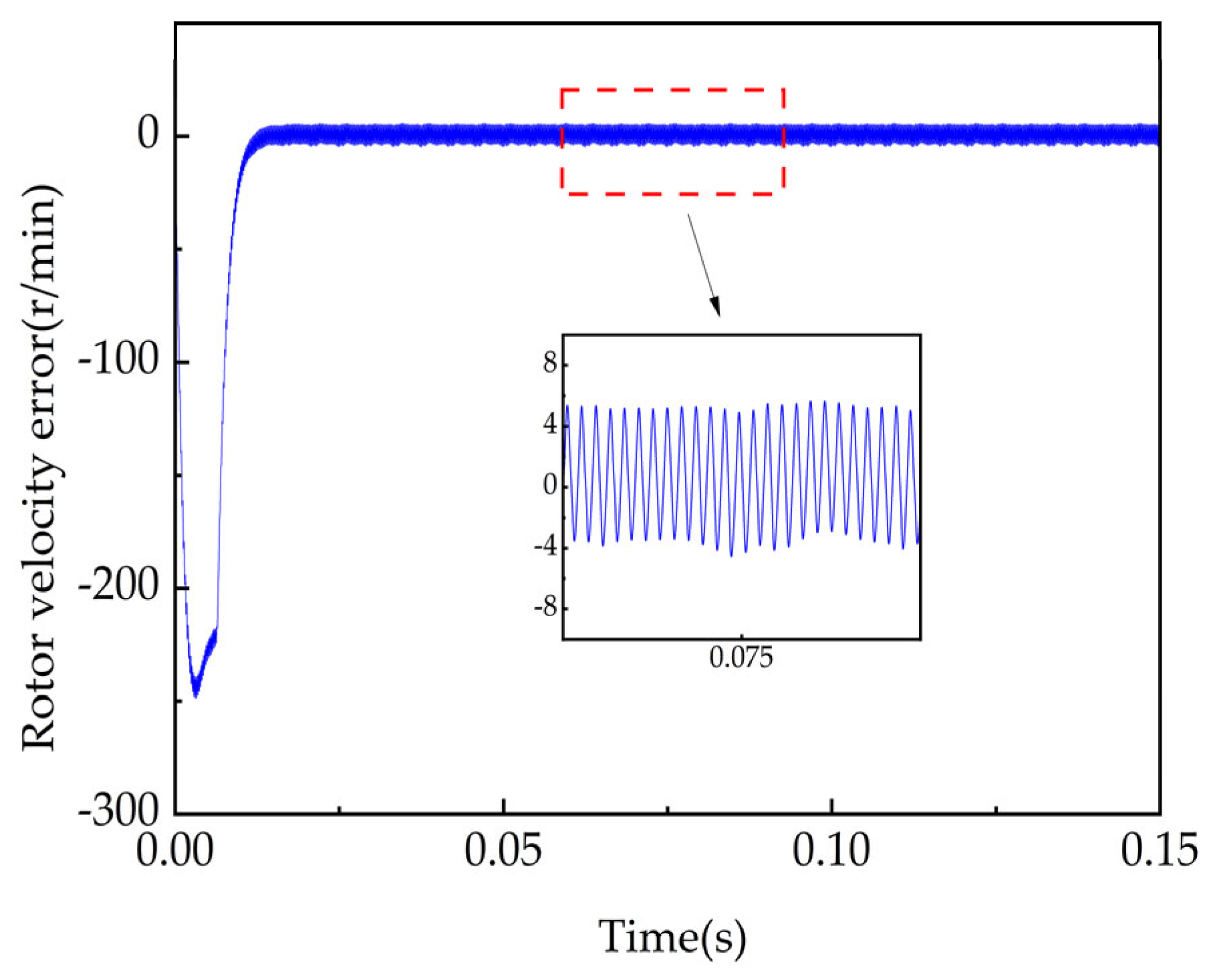
4.2. Analysis of Rotor Velocity Error and Rotor Position Error

Figure 10 and Figure 11 show the rotor velocity error results of the traditional SMO algorithm and the second-order adaptive SMO algorithm in the given conditions. Figure 12 and Figure 13 show the rotor position error results of the two algorithms.

From the four figures above, it can be seen that the rotor velocity error of the traditional SMO algorithm was 8.95 r/min and the rotor position error was 0.043 rad at 800 r/min, while in the same case, the rotor velocity error obtained by the second-order adaptive SMO algorithm was 0.57 r/min and the rotor position error was 0.018 rad, with accuracy improvements of 93.63% and 58.34%, respectively. When the rotor velocity increased to 1000 r/min, the rotor velocity error of the traditional SMO algorithm was 9.95 r/min and the rotor position error was 0.049 rad, while the rotor velocity error of the second-order adaptive SMO algorithm in the same case was 0.94 r/min and the rotor position error was 0.022 rad, with accuracy improvements of 90.55% and 55.10%, respectively. The results show that the second-order adaptive SMO algorithm had higher accuracy in estimating the rotor velocity and the rotor position, which effectively weakened the jitter phenomenon of the system.

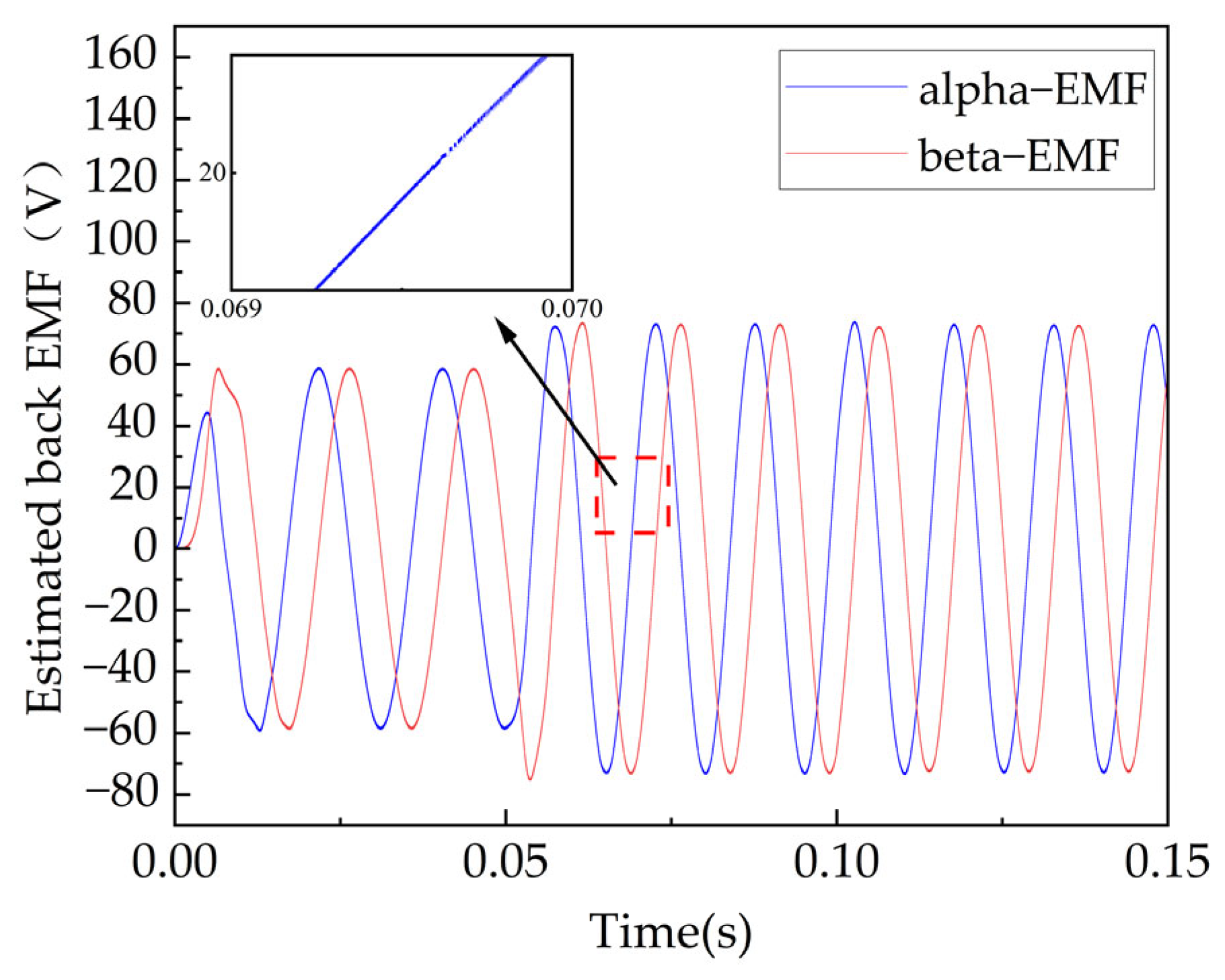
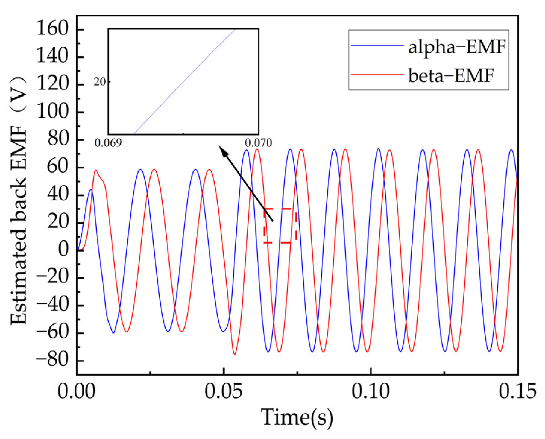
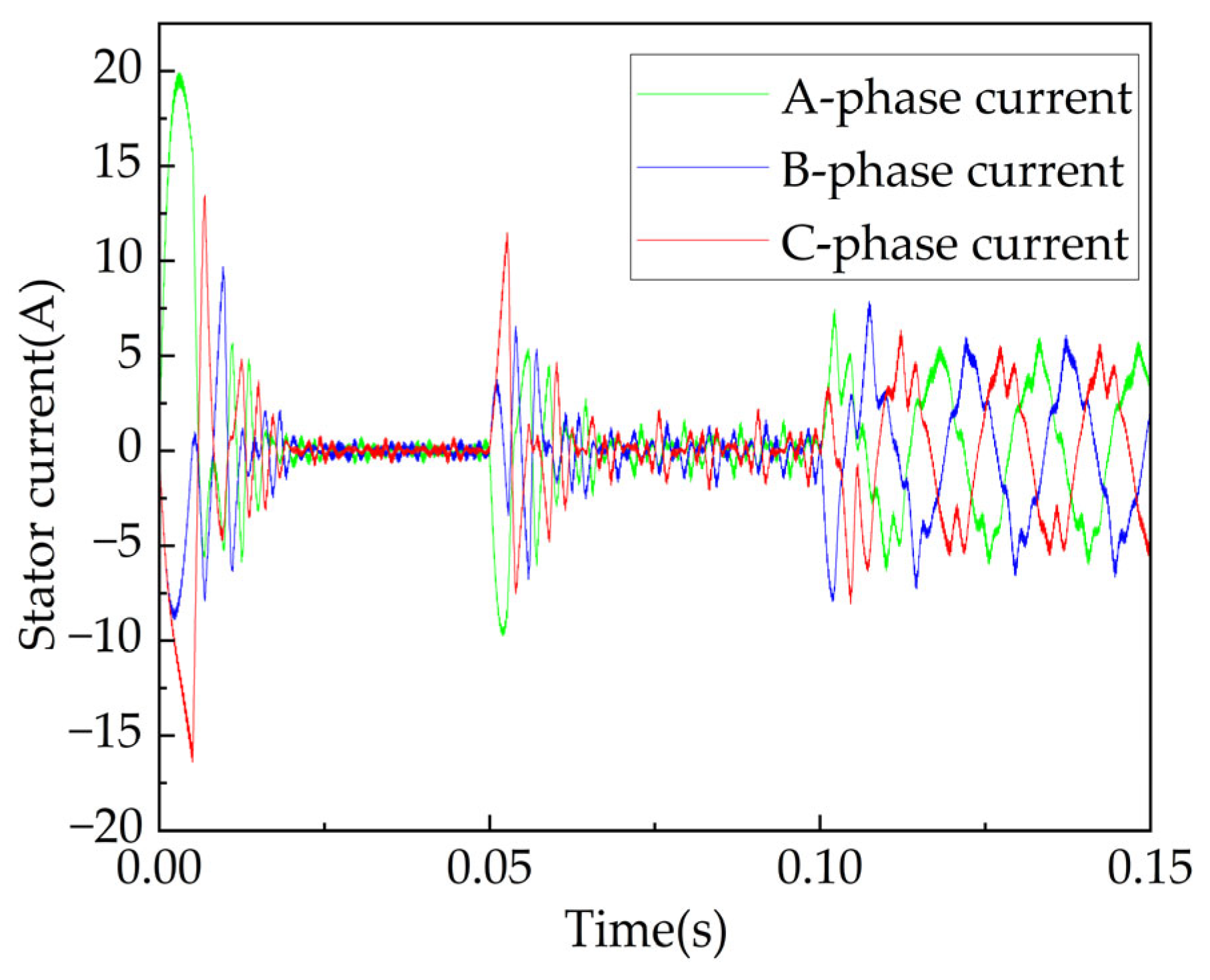
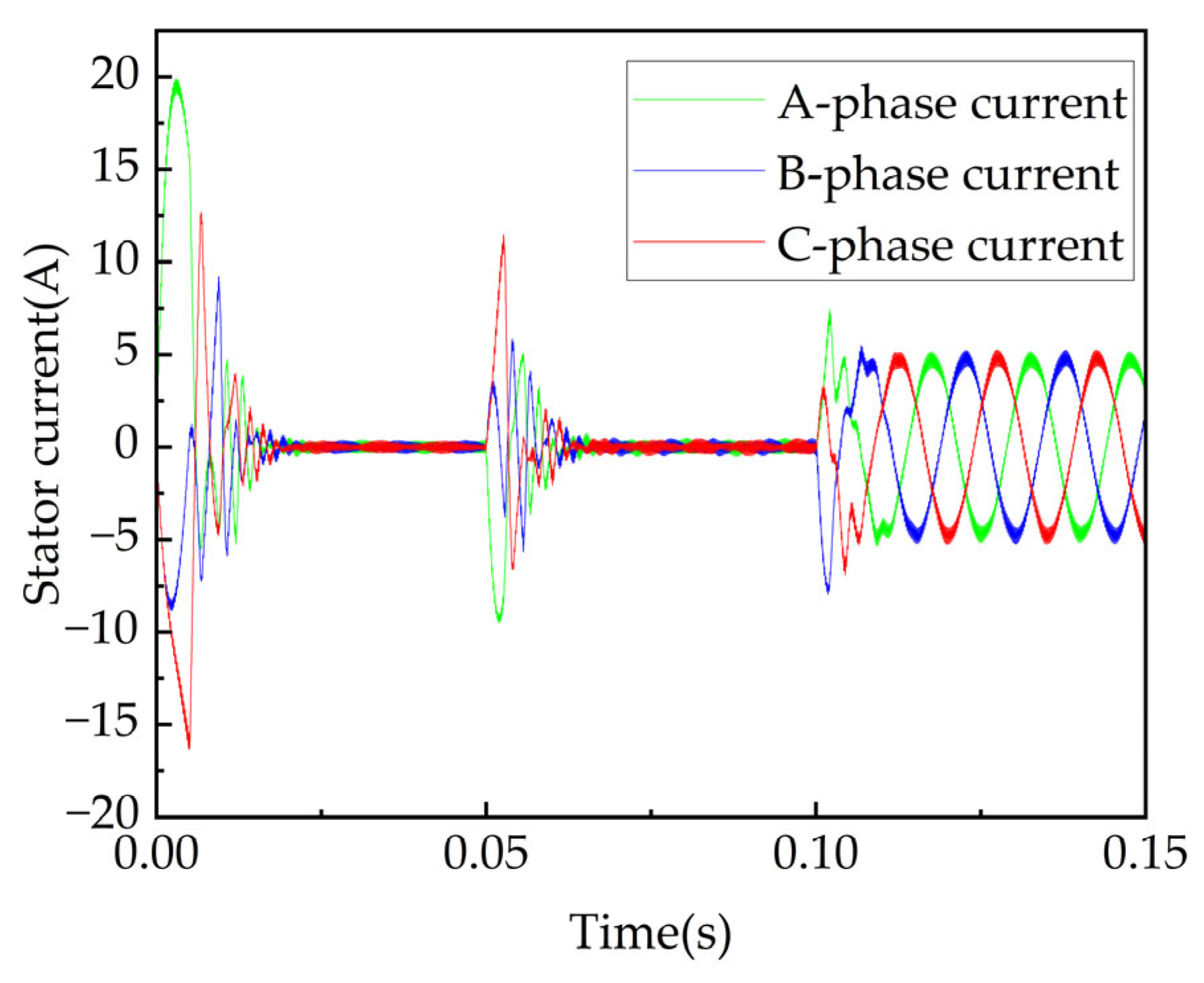
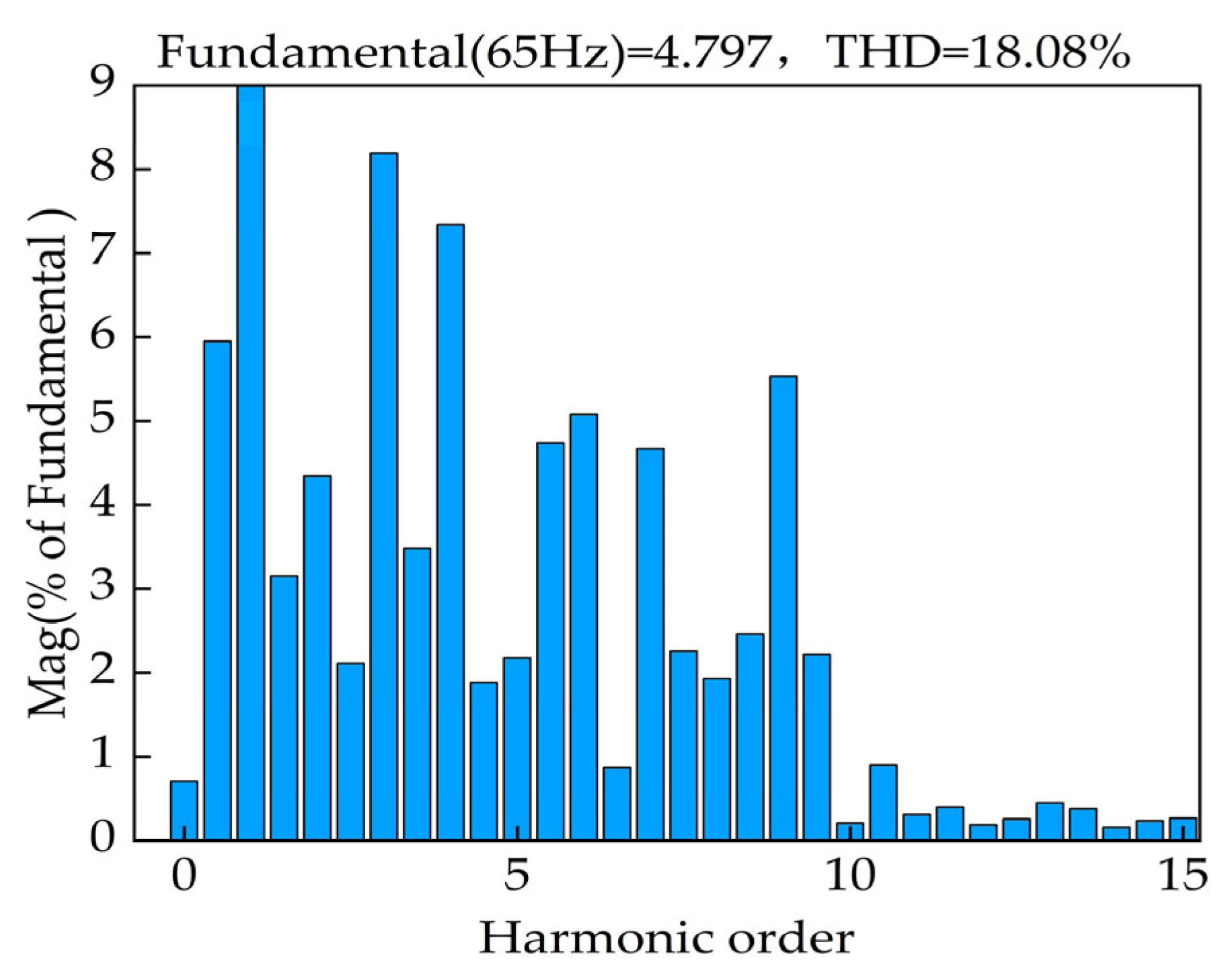
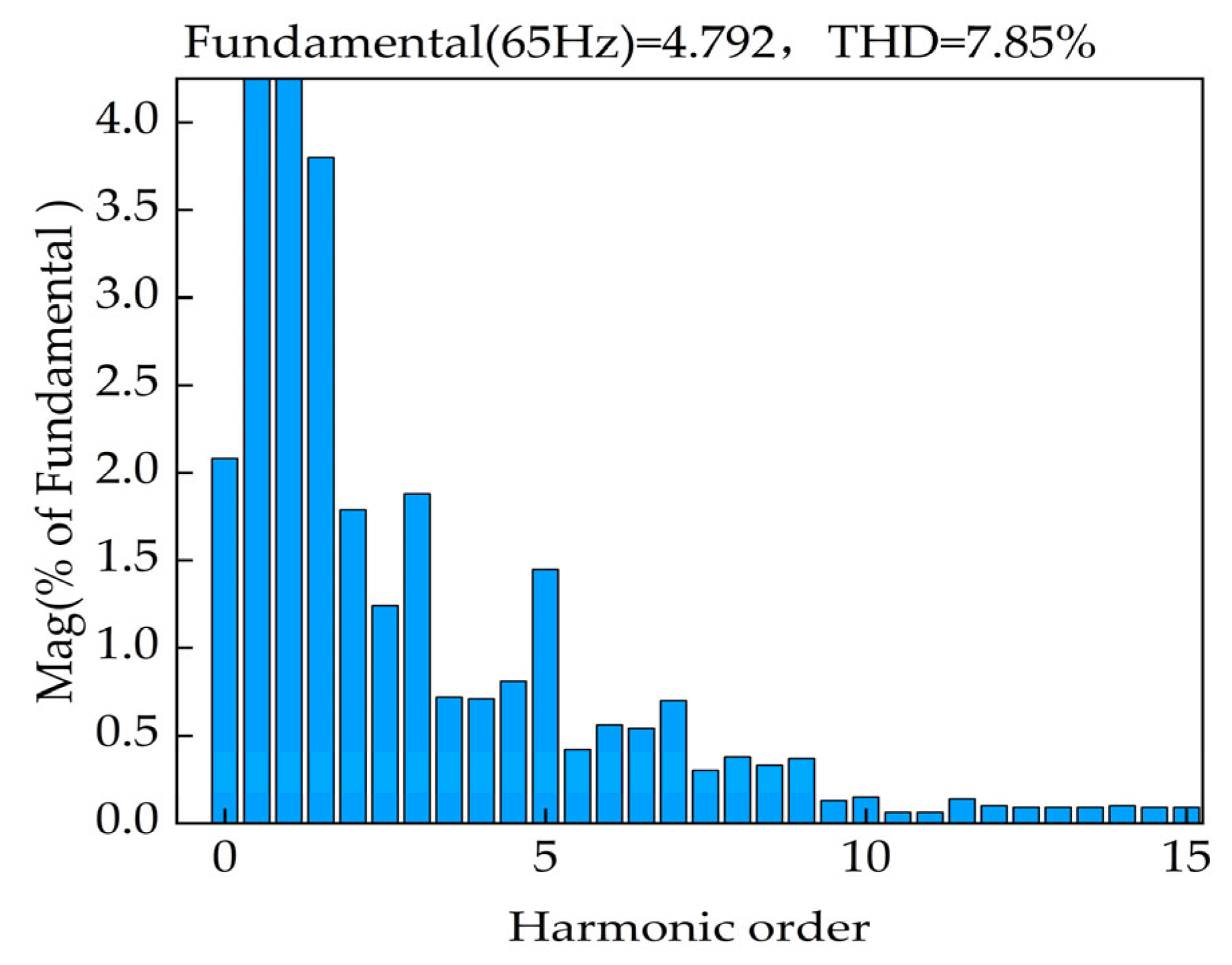
4.3. Analysis of the Estimated Back-EMF and the Three-Phase Current

Figure 14 and Figure 15 show the results of the estimated back-EMF for the traditional SMO algorithm and the second-order adaptive SMO algorithm in the given conditions. Figure 16 and Figure 17 show the three-phase current results of the two algorithms in the same conditions. Figure 18 and Figure 19 show the fast Fourier transforms (FFTs) of the A-phase current based on the two algorithms.

It can be seen in Figure 14 and Figure 15 that both algorithms were able to estimate the back-EMF effectively and show sine and cosine trends. With the increase in velocity, the back-EMF accurately reflected the performance change characteristics of the motor. However, the amplified waveform shows that the estimated back-EMF waveform of the traditional SMO algorithm had more burrs, while the estimated back-EMF waveform of the second-order adaptive SMO algorithm was very smooth. Comparing Figure 16 and Figure 17, it can be seen that the three-phase current waveform of the second-order adaptive SMO algorithm was smoother than that of the traditional SMO algorithm, especially after the load torque went from 0 to 5 N·m. At this point, the A-phase currents in the two algorithms were taken for fast Fourier transforms (FFTs). As shown in Figure 18 and Figure 19, the second-order adaptive SMO algorithm had fewer higher-order harmonics of the A-phase current, and the total harmonic distortion (THD) was reduced from the 18.08% value obtained by the traditional SMO algorithm to 7.85%. Therefore, the three-phase current of the second-order adaptive SMO algorithm had less distortion and was closer to a sinusoidal waveform. The analysis above shows that the second-order adaptive SMO had less noise in the estimated back-EMF and was more resistant to sudden load changes.

4.4. Stability Analysis under Mismatch of Stator Resistance

In the practical application of a PMSM, the high velocity running of the rotor, the heating of the winding, or a change in the external environment may lead to an increase in the internal temperature of the motor, which will eventually lead to a change in the stator resistance value of the motor. However, the stator resistance value in the given algorithm is pre-set and is not updated in real time. Therefore, a change in stator resistance may affect the stability of the control system, resulting in abnormal operation of the motor. In order to further verify the feasibility and reliability of the second-order adaptive SMO algorithm, it was necessary to analyze the stability of the system when the stator resistance was mismatched. To distinguish this analysis from the analysis above, the motor was set to accelerate from a static start to the target velocity of 1200 r/min, and the stator resistance was changed to 1.5 times the original. Figure 20 and Figure 21 show the rotor velocity and the rotor velocity error of the second-order adaptive SMO algorithm when the stator resistance was 3 Ω. Figure 22 and Figure 23 show the rotor velocity and the rotor velocity error of the second-order adaptive SMO algorithm when the stator resistance was 4.5 Ω.

It can be clearly seen in Figure 20, Figure 21, Figure 22 and Figure 23 that when the stator resistance of the PMSM was 3 Ω, the estimated velocity of the second-order adaptive SMO algorithm could accurately follow the actual value. The motor could run stably around 1200 r/min, and the velocity error was only 1.5 r/min. When the stator resistance was 4.5 Ω (1.5 times the original), the tracking performance of the algorithm was poor in the beginning, and there was a large deviation between the estimated velocity and the actual value. At a certain moment, the maximum deviation could reach about 250 r/min, but around 0.01 s, the motor could also reach 1200 r/min and ran stably, achieving good tracking of the actual velocity. After stabilization, the velocity error was 5.5 r/min. To summarize, although the tracking effect of the latter was not as good as that of the former, the latter could still make the motor run stably, and the velocity error was kept within a reasonable range, so the second-order adaptive SMO algorithm had high robustness.

4.5. Comparison of Results of Different Control Methods

The second-order adaptive SMO algorithm proposed in this paper was compared with other position-sensorless control algorithms in the field of PMSM control to prove the advanced nature of the proposed method. For a target velocity within 1000 r/min, the rotor velocity errors and the rotor position errors of different control methods are shown in

Table 2. Comparison of different position-sensorless algorithms.

Data Source	Algorithm	Rotor Velocity Error (r/min)	Rotor Position Error (rad)
Reference [32]	An improved SMO based on tanh(x)	1	0.05
Reference [33]	Fuzzy SMO	2	-
Reference [34]	Sensorless control based on PLL	5	0.087
Reference [35]	A novel MRAS algorithm	1.5	-
This paper	Traditional SMO	9.95	0.049
This paper	Second-order adaptive SMO	0.94	0.022

below. As can be seen in the table, the algorithms can accurately obtain the velocity and position information of a rotor, but compared with the other algorithms, the second-order adaptive SMO algorithm has smaller error and a better control effect.

5. Conclusions

In this paper, a second-order adaptive SMO algorithm was proposed. Through the second-order algorithm, the high-frequency switching term appeared in the observer in the form of an integral. At the same time, the adaptive estimation of back-EMF was introduced, and the back-EMF of the motor was estimated with the participation of the electrical angular velocity. This algorithm can track the phase of a PMSM instead of using mechanical sensors to obtain the rotor position and rotor velocity information of the motor. The following findings were obtained from the above analysis:

(1)

This algorithm effectively weakens the jitter of the traditional SMO algorithm, reduces the velocity error and position error, and improves the velocity and position tracking performance of the system.

(2)

The estimated back-EMF noise is smaller, and there are fewer high-order harmonics of the current after adding load, making this algorithm more resistant to sudden load changes and giving it high robustness.

(3)

Compared with other PMSM position-sensorless control algorithms, the estimation accuracy of rotor velocity and position of the algorithm proposed in this paper is higher.

In summary, the second-order adaptive SMO algorithm has good stability, feasibility, and reliability, which can meet the requirements of a high-precision PMSM position-sensorless control system and make the controlled motor have good performance. However, the research in this paper is only applicable at a medium–high velocity, and the estimation accuracy of the rotor velocity and position is not high enough when the velocity is too low. In future research, the control algorithm of the motor will continue to be optimized. A composite control strategy can be considered, where different control algorithms are adopted at zero–low velocity and at medium–high velocity. In addition, a switching velocity domain can be added in the middle, a weighted method can be used to realize the switching of the two control algorithms, and finally the stable operation of the motor in the full velocity domain can be realized.

References

1. Cao, Z.; Mahmoudi, A.; Kahourzade, S.; Soong, W.L. An Overview of Electric Motors for Electric Vehicles. In Proceedings of the 2021 31st Australasian Universities Power Engineering Conference (AUPEC), Perth, Australia, 26–30 September 2021; pp. 1–6. [Google Scholar]
2. Huang, S.; Ching, T.W.; Li, W.; Deng, B. Overview of Linear Motors for Transportation Applications. In Proceedings of the 2018 IEEE 27th International Symposium on Industrial Electronics (ISIE), Cairns, Australia, 12–15 June 2018; pp. 150–154. [Google Scholar]
3. Manoharan, S.; Palpandian, P.; Mahalakshmi, B.; Govindarai, V. A Review of Indian Scenario on Energy Conservation in Ceiling Fans Powered by BLDC Motors. In Proceedings of the 2021 Innovations in Power and Advanced Computing Technologies (i-PACT), Kuala Lumpur, Malaysia, 27–29 November 2021; pp. 1–7. [Google Scholar]
4. Sakunthala, S.; Kiranmayi, R.; Mandadi, P.N. A study on industrial motor drives: Comparison and applications of PMSM and BLDC motor drives. In Proceedings of the 2017 International Conference on Energy, Communication, Data Analytics and Soft Computing (ICECDS), Chennai, India, 1–2 August 2017; pp. 537–540. [Google Scholar]
5. Varshney, A.; Sharma, U.; Singh, B. A Grid Interactive Sensorless Synchronous Reluctance Motor Drive for Solar Powered Water Pump for Agriculture and Residential Applications. In Proceedings of the 2020 IEEE International Conference on Power Electronics, Drives and Energy Systems (PEDES), Jaipur, India, 16–19 December 2020; pp. 1–6. [Google Scholar] [CrossRef]
6. Wang, Y.; Bianchi, N.; Bolognani, S.; Alberti, L. Synchronous motors for traction applications. In Proceedings of the 2017 International Conference of Electrical and Electronic Technologies for Automotive, Turin, Italy, 15–16 June 2017; pp. 1–8. [Google Scholar]
7. Wang, H.; Leng, J. Summary on development of permanent magnet synchronous motor. In Proceedings of the 2018 Chinese Control and Decision Conference (CCDC), Shenyang, China, 9–11 June 2018; pp. 689–693. [Google Scholar]
8. Li, T.; Sun, X.; Lei, G.; Guo, Y.; Yang, Z.; Zhu, J. Finite-Control-Set Model Predictive Control of Permanent Magnet Synchronous Motor Drive Systems—An Overview. IEEE/CAA J. Automatic. 2022, 9, 2087–2105. [Google Scholar] [CrossRef]
9. Dandan, Q.; Yanan, J.; Shuyang, Z. The Study of Permanent Magnet Demagnetization in Permanent Magnet Synchronous Motor. In Proceedings of the 2021 IEEE International Conference on Advances in Electrical Engineering and Computer Applications (AEECA), Dalian, China, 27–28 August 2021; pp. 761–764. [Google Scholar]
10. Loganayaki, A.; Kumar, R.B. Permanent Magnet Synchronous Motor for Electric Vehicle Applications. In Proceedings of the 2019 5th International Conference on Advanced Computing & Communication Systems (ICACCS), Coimbatore, India, 15–16 March 2019; pp. 1064–1069. [Google Scholar]
11. Sun, X.; Cao, J.; Lei, G.; Guo, Y.; Zhu, J. Speed Sensorless Control for Permanent Magnet Synchronous Motors Based on Finite Position Set. IEEE Trans. Ind. Electron. 2020, 67, 6089–6100. [Google Scholar] [CrossRef]
12. Huang, J.; Zhu, X.; Li, Y.; Qi, G.; Wu, Y.; He, Y. A New Composite Sensorless Control Strategy for PMSM Used in Electric Vehicle. In Proceedings of the 2022 IEEE Transportation Electrification Conference and Expo, Haining, China, 28–31 October 2022; pp. 1–6. [Google Scholar]
13. Thiemann, P.; Mantala, C.; Mueller, T.; Strothmann, R.; Zhou, E. PMSM sensorless control with Direct Flux Control for all speeds. In Proceedings of the 3rd IEEE International Symposium on Sensorless Control for Electrical Drives (SLED 2012), Milwaukee, WI, USA, 21–22 September 2012; pp. 1–6. [Google Scholar]
14. Gao, J.; Liu, J.; Gong, C. A High-efficiency PMSM Sensorless Control Approach Based on MPC Controller. In Proceedings of the IECON 2018—44th Annual Conference of the IEEE Industrial Electronics Society, Washington, DC, USA; 2018; pp. 2171–2176. [Google Scholar]
15. Lee, H.; Lee, J. Design of Iterative Sliding Mode Observer for Sensorless PMSM Control. IEEE Trans. Control Syst. Technol. 2013, 21, 1394–1399. [Google Scholar] [CrossRef]
16. Sun, P.; Ge, Q.; Zhang, B.; Wang, X. Sensorless Control Technique of PMSM Based on RLS On-Line Parameter Identification. In Proceedings of the 2018 21st International Conference on Electrical Machines and Systems (ICEMS), Jeju, Republic of Korea, 7–10 October 2018; pp. 1670–1673. [Google Scholar]
17. Li, H.; Zhang, X.; Xu, C.; Hong, J. Sensorless Control of IPMSM Using Moving-Average-Filter Based PLL on HF Pulsating Signal Injection Method. IEEE Trans. Energy Convers. 2020, 35, 43–52. [Google Scholar] [CrossRef]
18. Wu, M.; Xuan, X.; Chen, X. Sensorless estimation and simulation of PMSM based on high-frequency signal injection. In Proceedings of the 10th World Congress on Intelligent Control and Automation, Beijing, China, 6–8 July 2012; pp. 3438–3442. [Google Scholar] [CrossRef]
19. Suman, K.; Mathew, A.T. Speed Control of Permanent Magnet Synchronous Motor Drive System Using PI, PID, SMC and SMC plus PID Controller. In Proceedings of the 2018 International Conference on Advances in Computing, Communications and Informatics (ICACCI), Bangalore, India, 19–22 September 2018; pp. 543–549. [Google Scholar]
20. Zhang, H.-W.; Jiang, D.; Wang, X.-H.; Wang, M.-R. Direct Torque Sensorless Control of PMSM Based on Dual Extended Kalman Filter. In Proceedings of the 2021 33rd Chinese Control and Decision Conference (CCDC), Kunming, China, 22–24 May 2021; pp. 7499–7504. [Google Scholar]
21. Xiong, Y.; Wang, A.; Zhang, T. Sensor-Less Complex System Control of PMSM Based on Improved SMO. In Proceedings of the 2021 6th International Conference on Automation, Control and Robotics Engineering (CACRE), Dalian, China, 15–17 July 2021; pp. 228–232. [Google Scholar]
22. Saadaoui, O.; Khlaief, A.; Abassi, M.; Chaari, A.; Boussak, M. Position sensorless vector control of PMSM drives based on SMO. In Proceedings of the 2015 16th International Conference on Sciences and Techniques of Automatic Control and Computer Engineering (STA), Monastir, Tunisia, 21–23 December 2015; pp. 545–550. [Google Scholar]
23. Badini, S.S.; Verma, V. A Novel MRAS Based Speed Sensorless Vector Controlled PMSM Drive. In Proceedings of the 2019 54th International Universities Power Engineering Conference (UPEC), Bucharest, Romania, 3–6 September 2019; pp. 1–6. [Google Scholar]
24. Ni, Y.; Shao, D. Research of Improved MRAS Based Sensorless Control of Permanent Magnet Synchronous Motor Considering Parameter Sensitivity. In Proceedings of the 2021 IEEE 4th Advanced Information Management, Communicates, Electronic and Automation Control Conference (IMCEC), Chongqing, China, 18–20 June 2021; pp. 633–638. [Google Scholar] [CrossRef]
25. Bernardes, T.; Montagner, V.F.; Grundling, H.A.; Pinheiro, H. Discrete-Time Sliding Mode Observer for Sensorless Vector Control of Permanent Magnet Synchronous Machine. IEEE Trans. Ind. Electron. 2014, 61, 1679–1691. [Google Scholar] [CrossRef]
26. Ding, L.; Li, Y.W.; Zargari, N.R. Discrete-Time SMO Sensorless Control of Current Source Converter-Fed PMSM Drives with Low Switching Frequency. IEEE Trans. Ind. Electron. 2021, 68, 2120–2129. [Google Scholar] [CrossRef]
27. Jiang, T.; Ni, R.; Gu, S.; Wang, G. A Study on Position Estimation Error in Sensorless Control of PMSM Based on Back EMF Observation Method. In Proceedings of the 2021 24th International Conference on Electrical Machines and Systems (ICEMS), Gyeongju, Republic of Korea, 31 October–3 November 2021; pp. 1999–2003. [Google Scholar]
28. An, Q.; An, Q.; Liu, X.; Zhang, J.; Bi, K. Improved Sliding Mode Observer for Position Sensorless Control of Permanent Magnet Synchronous Motor. In Proceedings of the 2018 IEEE Transportation Electrification Conference and Expo, Asia-Pacific (ITEC Asia-Pacific), Bangkok, Thailand, 6–9 June 2018; pp. 1–7. [Google Scholar]
29. Gong, C.; Hu, Y.; Gao, J.; Wang, Y.; Yan, L. An Improved Delay-Suppressed Sliding-Mode Observer for Sensorless Vector-Controlled PMSM. IEEE Trans. Ind. Electron. 2020, 67, 5913–5923. [Google Scholar] [CrossRef]
30. Davila, J.; Fridman, L.; Levant, A. Second-order sliding-mode observer for mechanical systems. IEEE Trans. Autom. Control 2005, 50, 1785–1789. [Google Scholar] [CrossRef]
31. Moreno, J.A.; Osorio, M. A Lyapunov approach to second-order sliding mode controllers and observers. In Proceedings of the 2008 47th IEEE Conference on Decision and Control, Cancun, Mexico, 9–11 December 2008; pp. 2856–2861. [Google Scholar] [CrossRef]
32. Chen, K.; Song, B.; Xiao, Y.; Xu, L. An Improved Sliding Mode Observer for Sensorless Vector Control of PMSM—A Simulation Study. In Proceedings of the 2019 Chinese Automation Congress (CAC), Hangzhou, China, 22–24 November 2019; pp. 1912–1916. [Google Scholar]
33. Zhang, X.; Jiang, Q. Research on Sensorless Control of PMSM Based on Fuzzy Sliding Mode Observer. In Proceedings of the 2021 IEEE 16th Conference on Industrial Electronics and Applications (ICIEA), Chengdu, China, 1–4 August 2021; pp. 213–218. [Google Scholar]
34. Li, Z.; Zhao, X.; Wang, Y.; Yue, C.; Jiang, L. Implementation of a PMSM Sensorless Control Method based on PLL back EMF. In Proceedings of the 2021 33rd Chinese Control and Decision Conference (CCDC), Kunming, China, 22–24 May 2021; pp. 4916–4921. [Google Scholar]
35. Zhou, F.; Yang, J.; Li, B. A Novel Speed Observer Based on Parameter-optimized MRAS for PMSMs. In Proceedings of the 2008 IEEE International Conference on Networking, Sensing and Control, Sanya, China, 6–8 April 2008; pp. 1708–1713. [Google Scholar]
Figure 1. The physical model of a three-phase PMSM.
Processes 11 01636 g001
Figure 2. Structure diagram of the second-order SMO algorithm.
Processes 11 01636 g002
Figure 3. Structure diagram of the link of adaptive estimation of back-EMF.
Processes 11 01636 g003
Figure 4. Structure diagram of the second-order adaptive SMO algorithm.
Processes 11 01636 g004
Figure 5. Block diagram of the control system.
Processes 11 01636 g005
Figure 6. Rotor velocity of traditional SMO algorithm.
Processes 11 01636 g006
Figure 7. Rotor velocity of second-order adaptive SMO algorithm.
Processes 11 01636 g007
Figure 8. Rotor position of traditional SMO algorithm.
Processes 11 01636 g008
Figure 9. Rotor position of second-order adaptive SMO algorithm.
Processes 11 01636 g009
Figure 10. Rotor velocity error of traditional SMO algorithm.
Processes 11 01636 g010
Figure 11. Rotor velocity error of second-order adaptive SMO algorithm.
Processes 11 01636 g011
Figure 12. Rotor position error of traditional SMO algorithm.
Processes 11 01636 g012
Figure 13. Rotor position error of second-order adaptive SMO algorithm.
Processes 11 01636 g013
Figure 14. Estimated back-EMF of traditional SMO algorithm.
Processes 11 01636 g014
Figure 15. Estimated back-EMF of second-order adaptive SMO algorithm.
Processes 11 01636 g015
Figure 16. Three-phase current of traditional SMO algorithm.
Processes 11 01636 g016
Figure 17. Three-phase current of second-order adaptive SMO algorithm.
Processes 11 01636 g017
Figure 18. The FFT of the A-phase current based on the traditional SMO algorithm.
Processes 11 01636 g018
Figure 19. The FFT of the A-phase current based on the second-order adaptive SMO algorithm.
Processes 11 01636 g019
Figure 20. Rotor velocity of second-order adaptive SMO algorithm (Rs = 3 Ω).
Processes 11 01636 g020
Figure 21. Rotor velocity error of second-order adaptive SMO algorithm (Rs = 3 Ω).
Processes 11 01636 g021
Figure 22. Rotor velocity of second-order adaptive SMO algorithm (Rs = 4.5 Ω).
Processes 11 01636 g022
Figure 23. Rotor velocity error of second-order adaptive SMO algorithm (Rs = 4.5 Ω).
Processes 11 01636 g023