
Residence Time Section Evaluation and Feasibility Studies for One-Column Simulated Moving Bed Processes (1-SMB)

Abstract
:1. Introduction
2. Materials and Methods
2.1. Chromatography Columns, Buffers and Feed
2.2. Chromatography Modeling
2.2.1. General Rate Model
2.2.2. Mass Balance of Mobile Phase
2.2.3. Mass Balance of Stationary Phase
2.2.4. Adsorption Equilibrium
2.3. Model Parameter Determination
2.3.1. Fluid Dynamics
2.3.2. Adsorption Equilibrium
2.3.3. Mass Transport
2.3.4. Model Validation
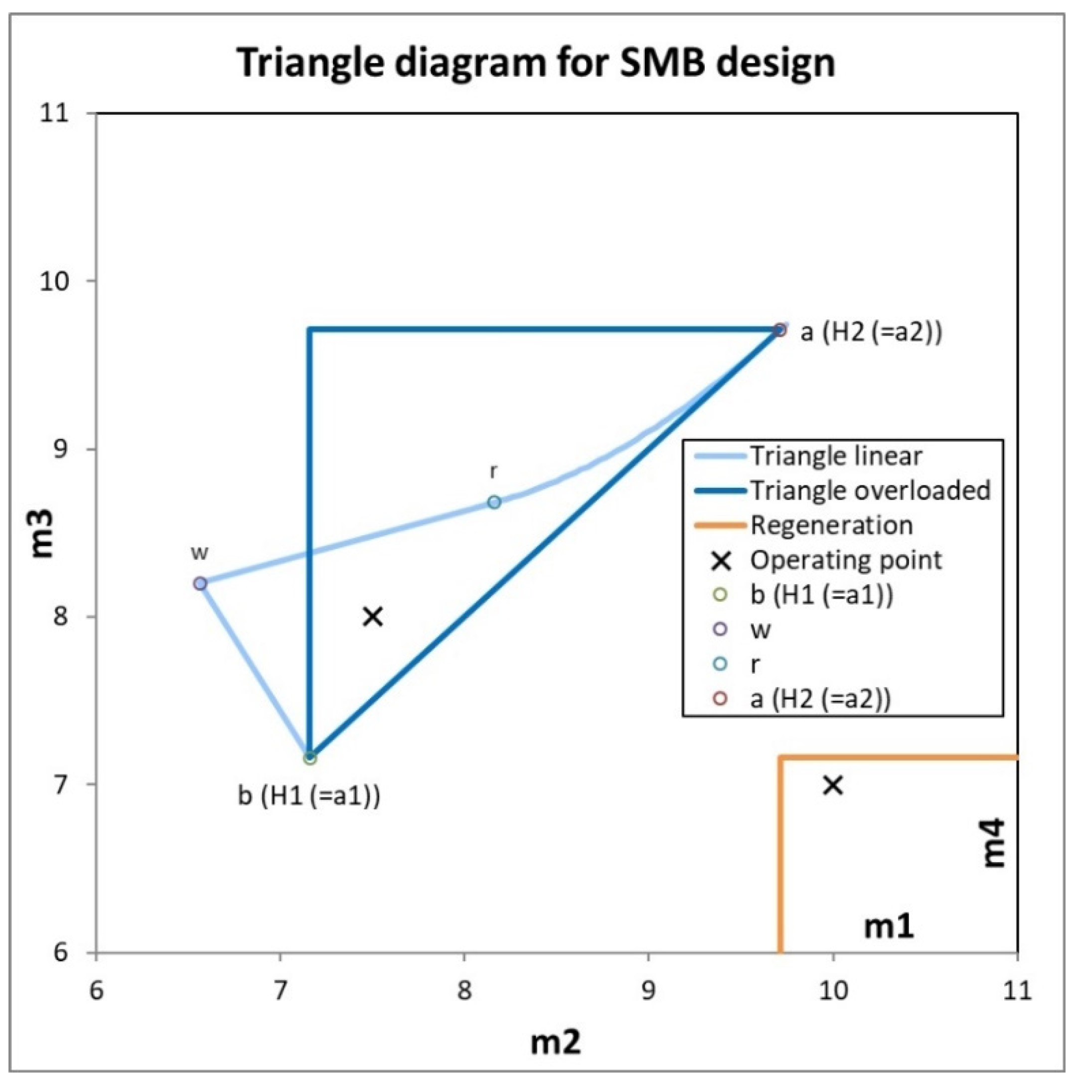
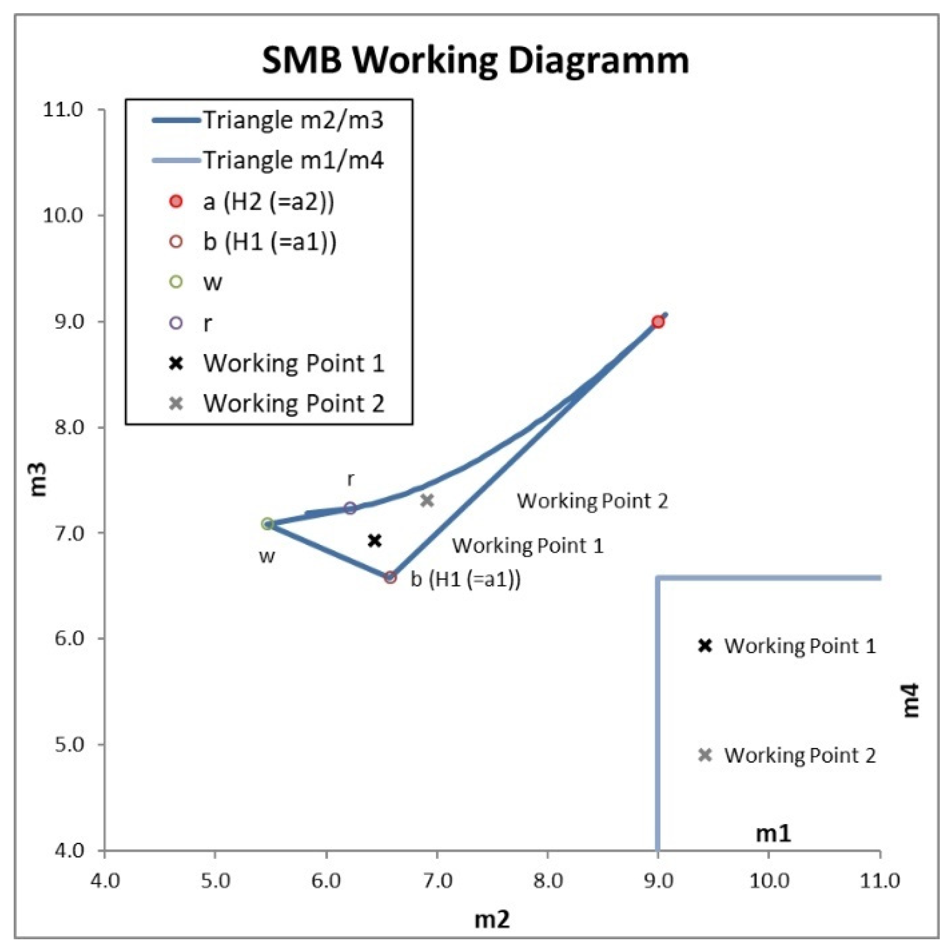
2.4. Triangle Theory
2.5. Axial Dispersion Coefficient for Residence Time Sections
3. Results and Discussion
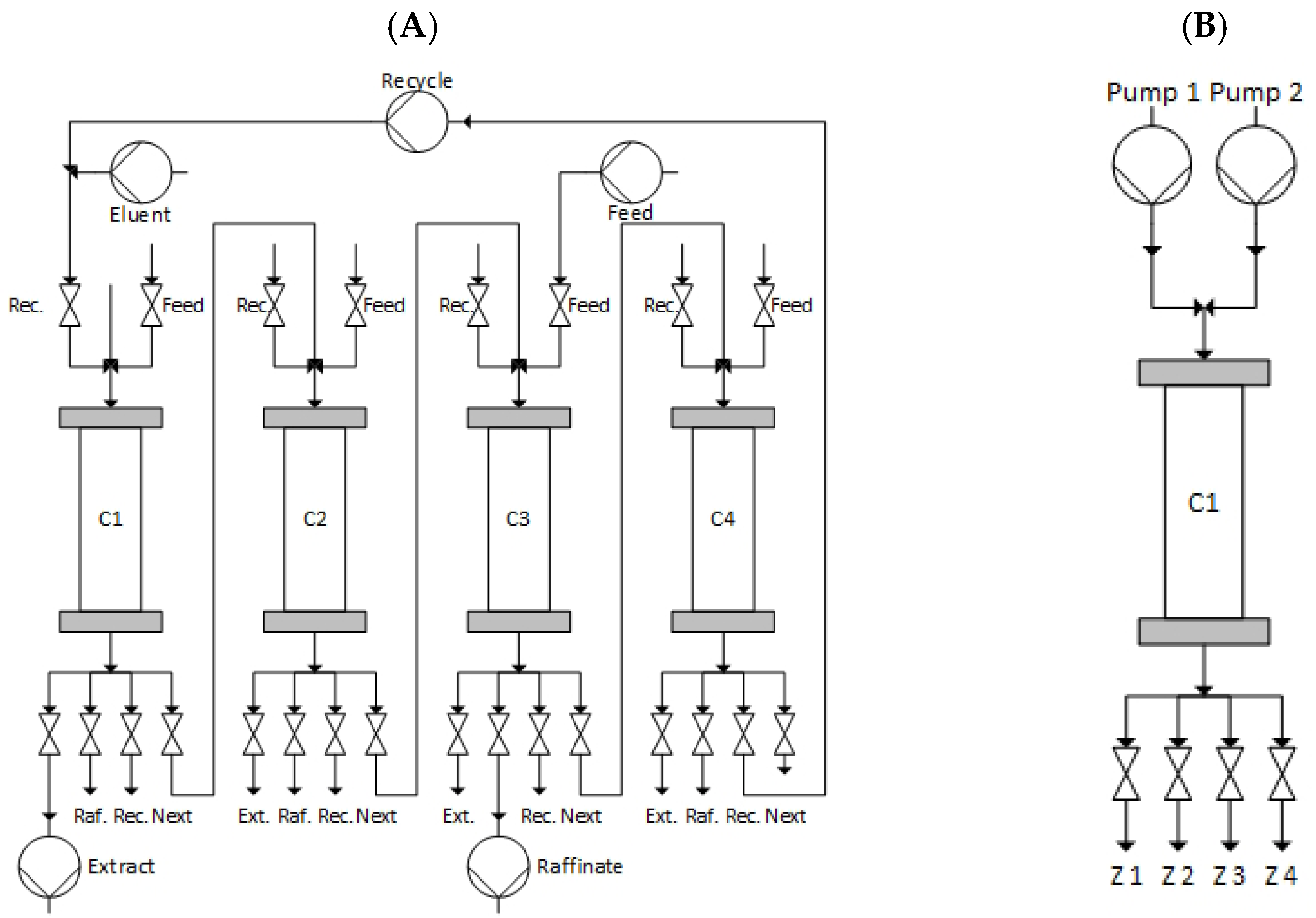
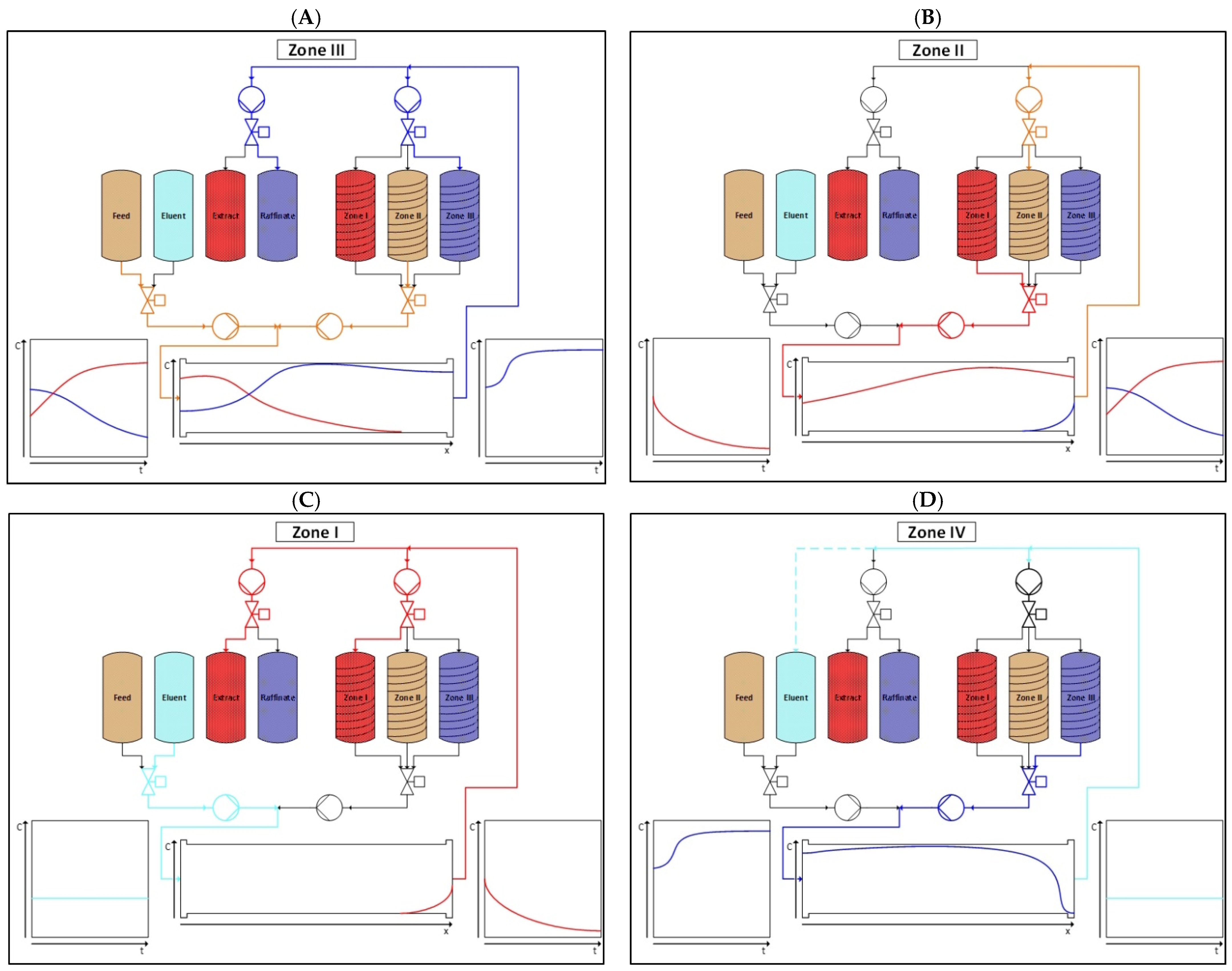
3.1. Simulated Moving Bed Design
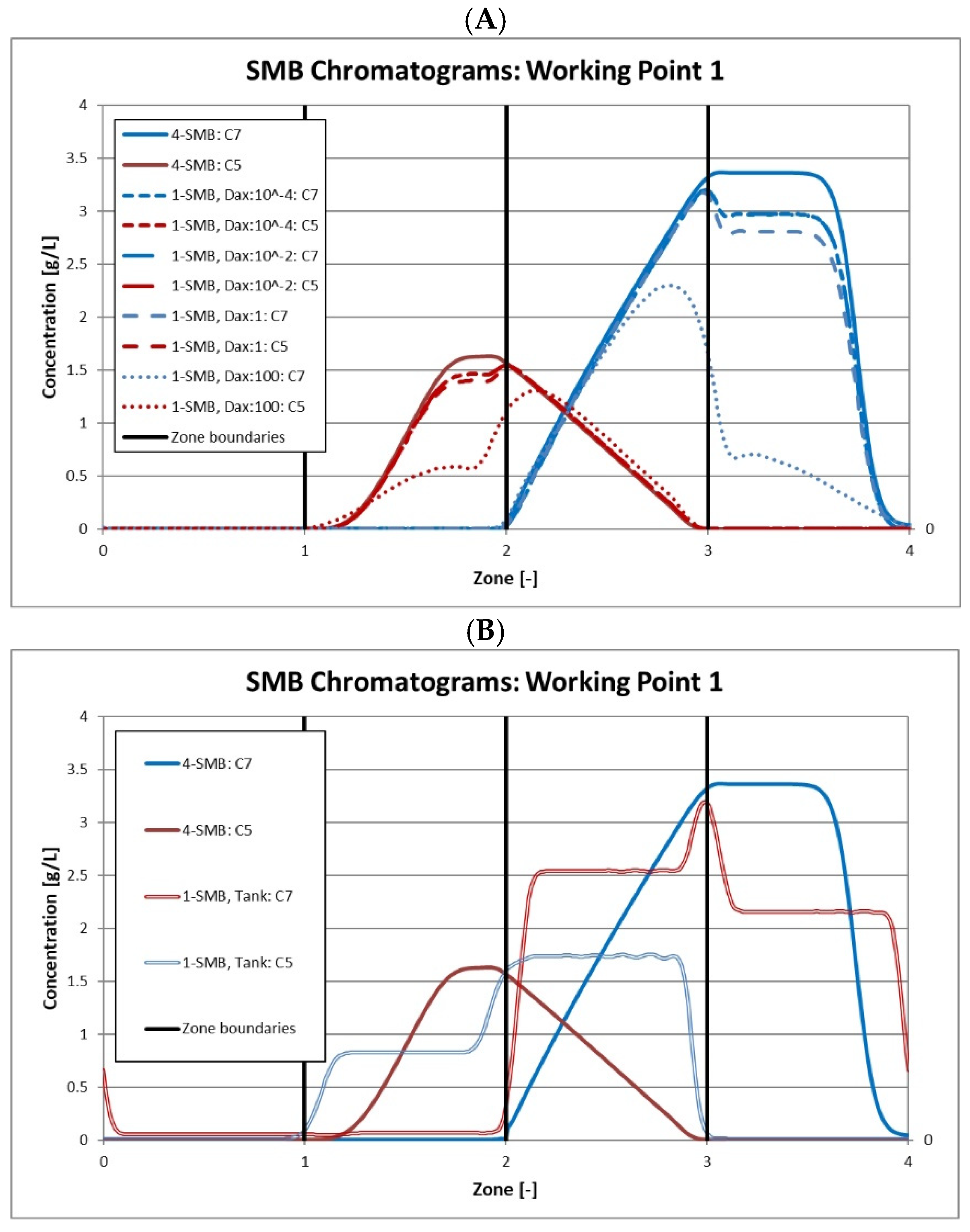
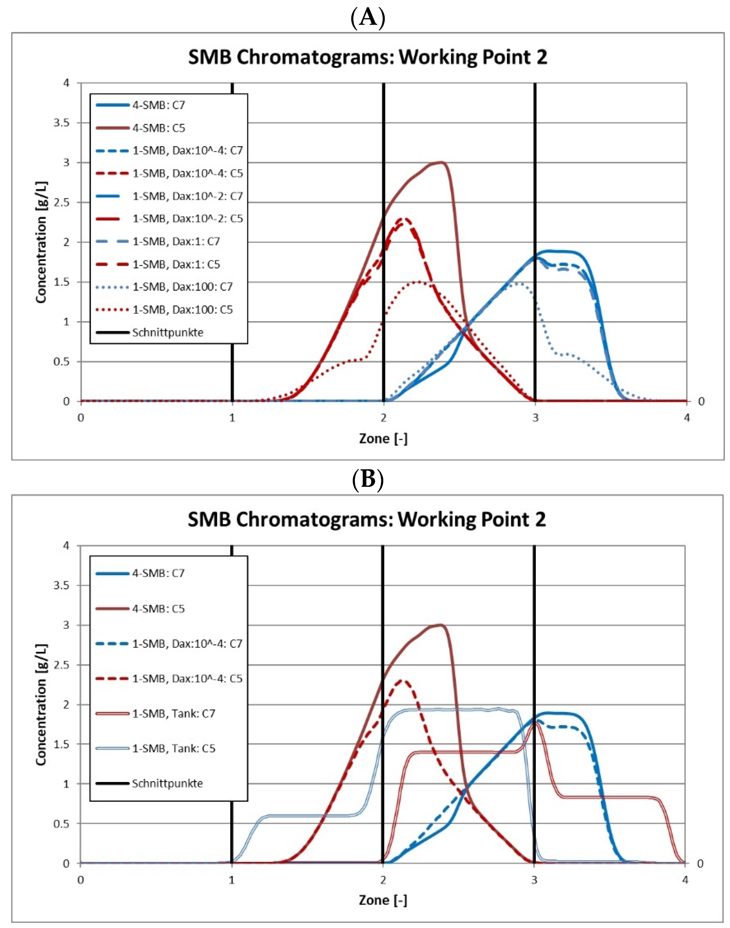
3.2. Simulation Studies
3.3. Retention Time Device Concepts
3.3.1. Coiled Flow Inverter (CFI)
3.3.2. Packed Bed Columns
3.3.3. Tank Cascades or Sequential Setups
3.3.4. Eluate Recycling Device
4. Conclusions
Author Contributions
Funding
Data Availability Statement
Acknowledgments
Conflicts of Interest
Abbreviations
| α | Selectivity | |
| (g/L) | Concentration of component i | |
| (g/L) | Concentration of component i inside the pores | |
| (cm2/s) | Axial dispersion coefficient | |
| Deff | (cm2/s) | Effective diffusion coefficient |
| (cm) | Particle diameter | |
| Dp,i | (cm2/s) | Pore diffusion coefficient |
| DS,i | (cm2/s) | Surface diffusion coefficient |
| (-) | Porosity | |
| (-) | Voidage | |
| (-) | Total porosity | |
| Hi | (-) | Henry coefficient of component i |
| Ki | (L/g) | Langmuir coefficient of component i |
| (cm/s) | Effective mass transport coefficient | |
| kf | (cm/s) | Mass transport coefficient |
| l | (cm) | Length |
| mj | Mass flow ratio of zone j | |
| n | Number of bends | |
| PAT | Process analytical technology | |
| qi | (g/L) | Loading of component i |
| qmax,i | (g/L) | Maximum loading capacity of component i |
| r | (cm) | Radius |
| Re | (-) | Reynolds number |
| (cm) | Particle radius | |
| Rs | Resolution | |
| t | (s); (min) | Time |
| t0 | (s); (min) | Dead time |
| tR1 | (s); (min) | Retention time peak 1 |
| tR2 | (s); (min) | Retention time peak 2 |
| (s); (min) | Mean residence time | |
| (cm/s) | Interstitial velocity | |
| v | (cm/s) | Velocity |
| (mL/min) | Volumetric flow | |
| (mL) | Volume of column | |
| (mg/cm*s) | Dynamic viscosity | |
| (g/L) | Density | |
| (s2) | Variance | |
| Mass fraction of component i | ||
| wb1 | (s); (min) | Peak width peak 1 |
| wb2 | (s); (min) | Peak width peak 1 |
References
- Strube, J. Technische Chromatographie: Auslegung, Optimierung, Betrieb und Wirtschaftlichkeit; Shaker: Aachen, Germany, 2000; ISBN 3826568974. [Google Scholar]
- Guiochon, G.; Felinger, A.; Shirazi, D.G.; Katti, A.M. Fundamentals of Preparative and Nonlinear Chromatography, 2nd ed.; Elsevier: Amsterdam, The Netherlands, 2006. [Google Scholar]
- Rodrigues, A. Simulated Moving Bed Technology: Principles, Design and Process Applications; Elsevier Science: Burlington, NJ, USA, 2015; ISBN 9780128020241. [Google Scholar]
- Zobel-Roos, S. Entwicklung, Modellierung und Validierung von Integrierten Kontinuierlichen Gegenstrom-Chromatographie-Prozessen, 1. Auflage; Shaker: Herzogenrath, Germany, 2018; ISBN 3844061878. [Google Scholar]
- Abunasser, N.; Wankat, P.C.; Kim, Y.-S.; Koo, Y.M. One-Column Chromatograph with Recycle Analogous to a Four-Zone Simulated Moving Bed. Ind. Eng. Chem. Res. 2003, 42, 5268–5279. [Google Scholar] [CrossRef]
- Mota, J.P.B.; Araújo, J.M.M. Single-column simulated-moving-bed process with recycle lag. AIChE J. 2005, 51, 1641–1653. [Google Scholar] [CrossRef]
- Zobel, S.; Helling, C.; Ditz, R.; Strube, J. Design and Operation of Continuous Countercurrent Chromatography in Biotechnological Production. Ind. Eng. Chem. Res. 2014, 53, 9169–9185. [Google Scholar] [CrossRef]
- Seidel-Morgenstern, A. Mathematische Modellierung der Präparativen Flüssigchromatographie; Deutscher Universitäts-Verlag: Wiesbaden, Germany, 1995; ISBN 3824420643. [Google Scholar]
- Abunasser, N.; Wankat, P. Ternary Separations with One-Column Analogs to SMB. Sep. Sci. Technol. 2005, 40, 3239–3259. [Google Scholar] [CrossRef]
- Abunasser, N.; Wankat, P.C. Improving the performance of one column analogs to SMBs. AIChE J. 2006, 52, 2461–2472. [Google Scholar] [CrossRef]
- de Araújo, J.M.; Rodrigues, R.C.; Silva, R.; Mota, J. Single-Column Simulated Moving-Bed Process with Recycle Lag: Analysis and Applications. Adsorpt. Sci. Technol. 2007, 25, 647–659. [Google Scholar] [CrossRef]
- Chibério, A.S.; Policarpo, G.F.; Antunes, J.C.; Santos, T.P.; Ribeiro, R.P.; Mota, J.P. Batch chromatography with recycle lag. II—Physical realization and experimental validation. J. Chromatogr. A 2020, 1623, 461211. [Google Scholar] [CrossRef]
- Chibério, A.S.; Santos, T.P.; Ribeiro, R.P.; Mota, J.P. Batch chromatography with recycle lag. I—Concept and design. J. Chromatogr. A 2020, 1623, 461199. [Google Scholar] [CrossRef]
- Juza, M. Development of a high-performance liquid chromatographic simulated moving bed separation from an industrial perspective. J. Chromatogr. A 1999, 865, 35–49. [Google Scholar] [CrossRef]
- Mazzotti, M. Equilibrium theory based design of simulated moving bed processes for a generalized Langmuir isotherm. J. Chromatogr. A 2006, 1126, 311–322. [Google Scholar] [CrossRef]
- Mazzotti, M.; Storti, G.; Morbidelli, M. Robust design of countercurrent adsorption separation processes: 2. Multicomponent systems. AIChE J. 1994, 40, 1825–1842. [Google Scholar] [CrossRef]
- Mazzotti, M.; Storti, G.; Morbidelli, M. Robust design of countercurrent adsorption separation: 3. Nonstoichiometric systems. AIChE J. 1996, 42, 2784–2796. [Google Scholar] [CrossRef]
- Mazzotti, M.; Storti, G.; Morbidelli, M. Optimal operation of simulated moving bed units for nonlinear chromatographic separations. J. Chromatogr. A 1997, 769, 3–24. [Google Scholar] [CrossRef]
- Mazzotti, M.; Storti, G.; Morbidelli, M. Robust design of countercurrent adsorption separation processes: 4. Desorbent in the feed. AIChE J. 1997, 43, 64–72. [Google Scholar] [CrossRef]
- Storti, G.; Baciocchi, R.; Mazzotti, M.; Morbidelli, M. Design of Optimal Operating Conditions of Simulated Moving Bed Adsorptive Separation Units. Ind. Eng. Chem. Res. 1995, 34, 288–301. [Google Scholar] [CrossRef]
- Storti, G.; Mazzotti, M.; Morbidelli, M.; Carrà, S. Robust design of binary countercurrent adsorption separation processes. AIChE J. 1993, 39, 471–492. [Google Scholar] [CrossRef]
- Zobel-Roos, S.; Mouellef, M.; Ditz, R.; Strube, J. Distinct and Quantitative Validation Method for Predictive Process Modelling in Preparative Chromatography of Synthetic and Bio-Based Feed Mixtures following a Quality-by-Design (QbD) Approach. Processes 2019, 7, 580. [Google Scholar] [CrossRef]
- Kaczmarski, K.; Cavazzini, A.; Szabelski, P.; Zhou, D.; Liu, X.; Guiochon, G. Application of the general rate model and the generalized Maxwell–Stefan equation to the study of the mass transfer kinetics of a pair of enantiomers. J. Chromatogr. A 2002, 962, 57–67. [Google Scholar] [CrossRef]
- Kaczmarski, K.; Gubernak, M.; Zhou, D.; Guiochon, G. Application of the general rate model with the Maxwell–Stefan equations for the prediction of the band profiles of the 1-indanol enantiomers. Chem. Eng. Sci. 2003, 58, 2325–2338. [Google Scholar] [CrossRef]
- Felinger, A.; Guiochon, G. Comparison of the Kinetic Models of Linear Chromatography. Chromatographia 2004, 60, S175–S180. [Google Scholar] [CrossRef]
- Piątkowski, W.; Antos, D.; Kaczmarski, K. Modeling of preparative chromatography processes with slow intraparticle mass transport kinetics. J. Chromatogr. A 2003, 988, 219–231. [Google Scholar] [CrossRef]
- Carta, G.; Jungbauer, A. Protein Chromatography: Process Development and Scale-Up; WILEY-VCH: Weinheim, Germany, 2010; ISBN 978-3-527-31819-3. [Google Scholar]
- Seidel-Morgenstern, A. Experimental determination of single solute and competitive adsorption isotherms. J. Chromatogr. A 2004, 1037, 255–272. [Google Scholar] [CrossRef]
- Asnin, L. Adsorption models in chiral chromatography. J. Chromatogr. A 2012, 1269, 3–25. [Google Scholar] [CrossRef] [PubMed]
- Blümel, C.; Kniep, H.; Seidel-Morgenstern, A. Measuring adsorption isotherms using a closed-loop perturbation method to minimize sample consumption. In 6th International Conference of Fundamentals of Adsorption—FOA 6; Elsevier: Amsterdam, The Netherlands, 1998; pp. 449–454. [Google Scholar]
- Cavazzini, A.; Felinger, A.; Guiochon, G. Comparison between adsorption isotherm determination techniques and overloaded band profiles on four batches of monolithic columns. J. Chromatogr. A 2003, 1012, 139–149. [Google Scholar] [CrossRef] [PubMed]
- Ching, C.B.; Chu, K.H.; Ruthven, D.M. A study of multicomponent adsorption equilibria by liquid chromatography. AIChE J. 1990, 36, 275–281. [Google Scholar] [CrossRef]
- Gamba, G.; Rota, R.; Storti, G.; Carra, S.; Morbidelli, M. Absorbed solution theory models for multicomponent adsorption equilibria. AIChE J. 1989, 35, 959–966. [Google Scholar] [CrossRef]
- Hu, X.; Do, D.D. Comparing various multicomponent adsorption equilibrium models. AIChE J. 1995, 41, 1585–1592. [Google Scholar] [CrossRef]
- Heinonen, J.; Landa, H.O.R.; Sainio, T.; Seidel-Morgenstern, A. Use of Adsorbed Solution theory to model competitive and co-operative sorption on elastic ion exchange resins. Sep. Purif. Technol. 2012, 95, 235–247. [Google Scholar] [CrossRef]
- Emerton, D.A. Profitability in the Biosimilars Market: Can You Translate Scientific Excellence into a Healthy Commercial Return? BioProcess Int. 2013, 11, 6–23. [Google Scholar]
- Erto, A.; Lancia, A.; Musmarra, D. A modelling analysis of PCE/TCE mixture adsorption based on Ideal Adsorbed Solution Theory. Sep. Purif. Technol. 2011, 80, 140–147. [Google Scholar] [CrossRef]
- Myers, A.L.; Prausnitz, J.M. Thermodynamics of mixed-gas adsorption. AIChE J. 1965, 11, 121–127. [Google Scholar] [CrossRef]
- Costa, E.; Calleja, G.; Marron, C.; Jimenez, A.; Pau, J. Equilibrium adsorption of methane, ethane, ethylene, and propylene and their mixtures on activated carbon. J. Chem. Eng. Data 1989, 34, 156–160. [Google Scholar] [CrossRef]
- Brooks, C.A.; Cramer, S.M. Steric mass-action ion exchange: Displacement profiles and induced salt gradients. AIChE J. 1992, 38, 1969–1978. [Google Scholar] [CrossRef]
- Langmuir, I. The adsorption of gases on plane surfaces of glass, mica and platinum. J. Am. Chem. Soc. 1918, 40, 1361–1403. [Google Scholar] [CrossRef]
- Zobel-Roos, S.; Schmidt, A.; Mestmäcker, F.; Mouellef, M.; Huter, M.; Uhlenbrock, L.; Kornecki, M.; Lohmann, L.; Ditz, R.; Strube, J. Accelerating Biologics Manufacturing by Modeling or: Is Approval under the QbD and PAT Approaches Demanded by Authorities Acceptable without a Digital-Twin? Processes 2019, 7, 94. [Google Scholar] [CrossRef]
- Zobel-Roos, S.; Schmidt, A.; Uhlenbrock, L.; Ditz, R.; Köster, D.; Strube, J. Digital Twins in Biomanufacturing. In Digital Twins: Tools and Concepts for Smart Biomanufacturing; Herwig, C., Pörtner, R., Möller, J., Eds.; Springer: Cham, Switzerland, 2021; pp. 181–262. ISBN 978-3-030-71660-8. [Google Scholar]
- Levenspiel, O. Chemical Reaction Engineering, 3rd ed.; John Wiley & Sons: New York, NY, USA, 1998; ISBN 978-0471254249. [Google Scholar]
- Rhee, H.-K.; Aris, R.; Amundson, N.R. Multicomponent adsorption in continuous countercurrent exchangers. Philos. Trans. R. Soc. Lond. Ser. A Math. Phys. Sci. 1971, 269, 187–215. [Google Scholar] [CrossRef]
- Fanali, S. Editorial on “Simulated moving bed chromatography for the separation of enantiomers” by A. Rajendran, G. Paredes and M. Mazzotti. J. Chromatogr. A 2009, 1216, 708. [Google Scholar] [CrossRef] [PubMed]
- Storti, G.; Masi, M.; Carrà, S.; Morbidelli, M. Optimal design of multicomponent countercurrent adsorption separation processes involving nonlinear equilibria. Chem. Eng. Sci. 1989, 44, 1329–1345. [Google Scholar] [CrossRef]
- Kaspereit, M.; Seidel-Morgenstern, A. Auslegung der Regenerationszonen des SMB-Verfahrens. Chem. Ing. Tech. 2002, 74, 591–592. [Google Scholar] [CrossRef]
- Kaspereit, M.; Neupert, B. Vereinfachte Auslegung der simulierten Gegenstromchromatographie mittels des Hodographenraums. Chem. Ing. Tech. 2016, 88, 1628–1642. [Google Scholar] [CrossRef]
- Kaspereit, M.; Jandera, P.; Škavrada, M.; Seidel-Morgenstern, A. Impact of adsorption isotherm parameters on the performance of enantioseparation using simulated moving bed chromatography. J. Chromatogr. A 2001, 944, 249–262. [Google Scholar] [CrossRef] [PubMed]
- Saxena, A.K.; Nigam, K.D.P. Coiled configuration for flow inversion and its effect on residence time distribution. AIChE J. 1984, 30, 363–368. [Google Scholar] [CrossRef]
- Kumar, V.; Nigam, K. Numerical simulation of steady flow fields in coiled flow inverter. Int. J. Heat Mass Transf. 2005, 48, 4811–4828. [Google Scholar] [CrossRef]
- Chung, S.F.; Wen, C.Y. Longitudinal dispersion of liquid flowing through fixed and fluidized beds. AIChE J. 1968, 14, 857–866. [Google Scholar] [CrossRef]


| Point | m2 | m3 |
|---|---|---|
| a | ||
| b | ||
| r | ||
| w |
| Working Point 1 | Working Point 2 | |
|---|---|---|
| m1 | 9.4 | 10.1 |
| m2 | 6.4 | 6.9 |
| m3 | 6.9 | 7.3 |
| m4 | 5.9 | 4.9 |
| Purity | Yield Column | Yield Process | Productivity | Eluent Consumption | ||||||
|---|---|---|---|---|---|---|---|---|---|---|
| C5 | C7 | C5 | C7 | C5 | C7 | C5 | C7 | C5 | C7 | |
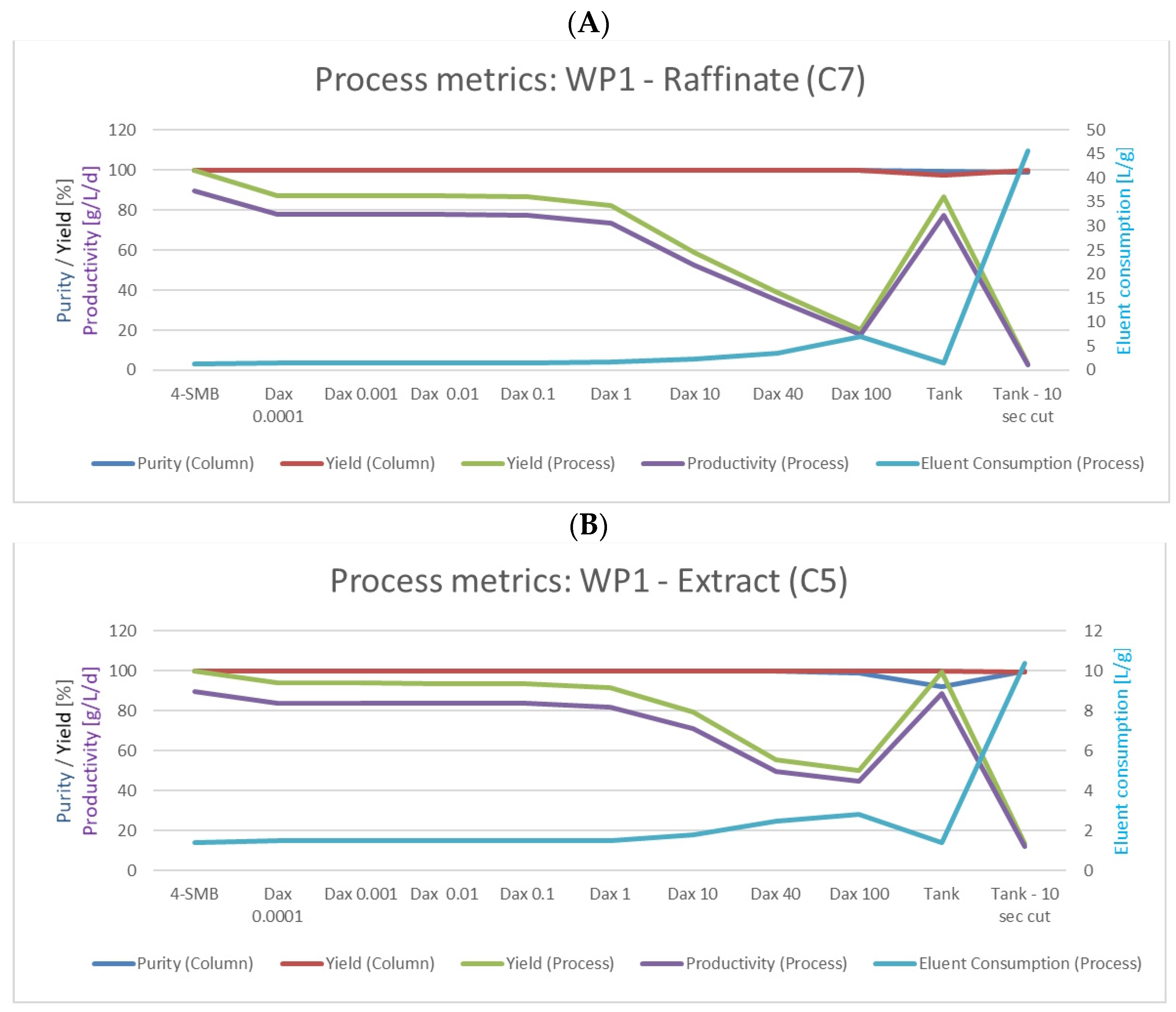
| 4-SMB | 100 | 100 | 100 | 100 | 100 | 100 | 89.5 | 89.5 | 1.4 | 1.4 |
| Dax 0.0001 | 99.9 | 100.0 | 100.0 | 100.0 | 93.9 | 87.1 | 84.0 | 78.0 | 1.5 | 1.6 |
| Dax 0.001 | 99.9 | 100.0 | 100.0 | 100.0 | 93.9 | 87.1 | 84.0 | 78.0 | 1.5 | 1.6 |
| Dax 0.01 | 99.9 | 100.0 | 100.0 | 100.0 | 93.8 | 87.0 | 84.0 | 77.9 | 1.5 | 1.6 |
| Dax 0.1 | 99.9 | 100.0 | 100.0 | 100.0 | 93.6 | 86.5 | 83.8 | 77.4 | 1.5 | 1.6 |
| Dax 1 | 99.9 | 100.0 | 100.0 | 100.0 | 91.5 | 82.0 | 81.9 | 73.4 | 1.5 | 1.7 |
| Dax 10 | 99.9 | 100.0 | 100.0 | 99.9 | 79.4 | 58.7 | 71.1 | 52.5 | 1.8 | 2.4 |
| Dax 40 | 99.9 | 100.0 | 100.0 | 99.9 | 55.5 | 38.7 | 49.7 | 34.7 | 2.5 | 3.6 |
| Dax 100 | 99.1 | 100.0 | 100.0 | 99.7 | 50.0 | 20.0 | 44.7 | 17.9 | 2.8 | 7.0 |
| Tank | 92.1 | 99.4 | 99.8 | 97.4 | 99.3 | 86.5 | 88.9 | 77.5 | 1.4 | 1.6 |
| Tank—10 sec cut | 99.9 | 98.9 | 99.6 | 100 | 13.5 | 3.1 | 12.1 | 2.7 | 10.4 | 45.7 |
| Purity | Yield Column | Yield Process | Productivity | Eluent Consumption | ||||||
|---|---|---|---|---|---|---|---|---|---|---|
| C5 | C7 | C5 | C7 | C5 | C7 | C5 | C7 | C5 | C7 | |
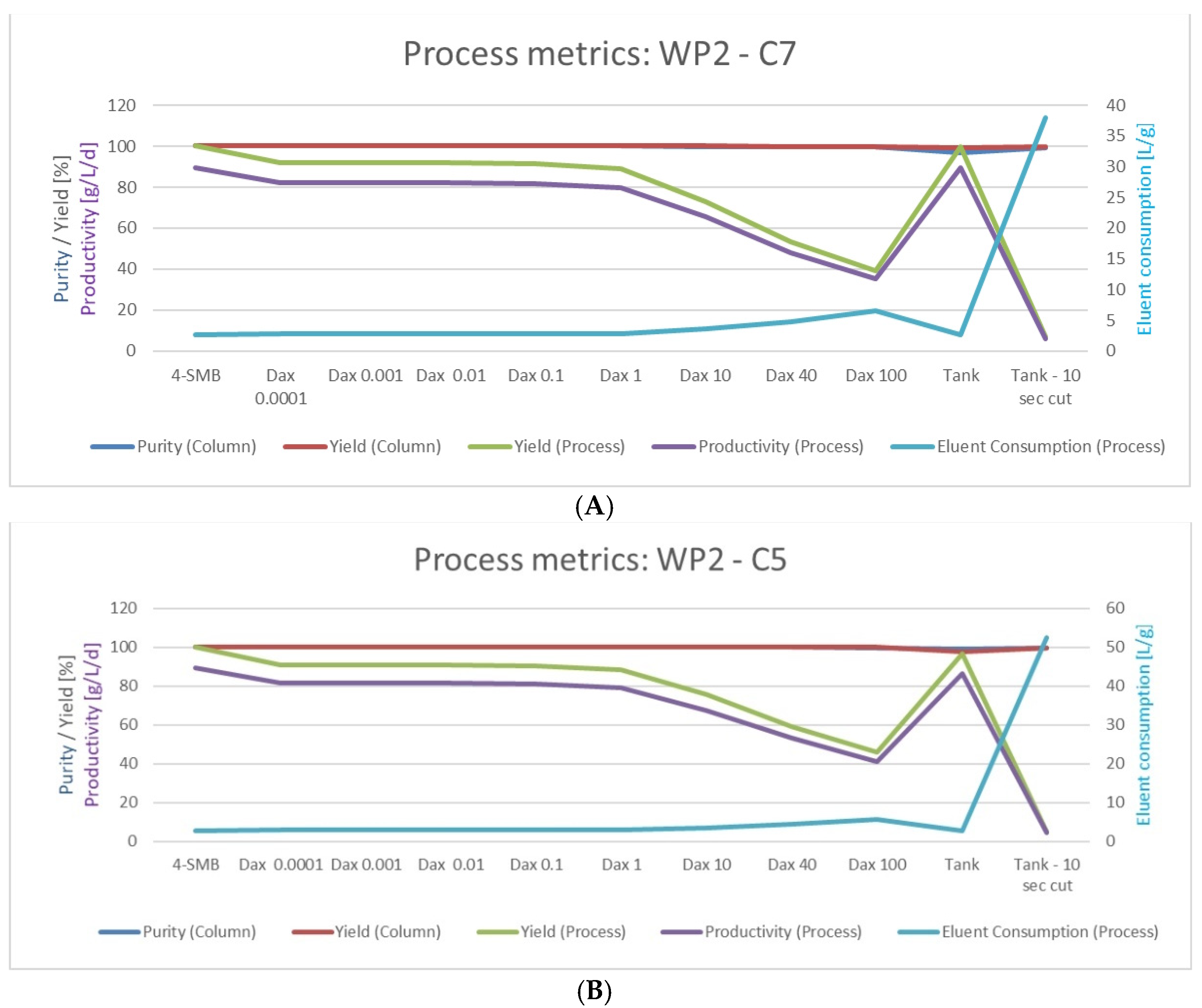
| 4-SMB | 100 | 100 | 100 | 100 | 100 | 100 | 89.5 | 89.5 | 2.6 | 2.6 |
| Dax 0.0001 | 100 | 100 | 100 | 100 | 90.9 | 91.8 | 81.4 | 82.2 | 2.9 | 2.8 |
| Dax 0.001 | 100 | 100 | 100 | 100 | 90.9 | 91.8 | 81.4 | 82.2 | 2.9 | 2.8 |
| Dax 0.01 | 100 | 100 | 100 | 100 | 90.9 | 91.8 | 81.4 | 82.2 | 2.9 | 2.8 |
| Dax 0.1 | 100 | 100 | 100 | 100 | 90.6 | 91.5 | 81.1 | 81.9 | 2.9 | 2.8 |
| Dax 1 | 100 | 100 | 100 | 100 | 88.4 | 88.8 | 79.2 | 79.5 | 2.9 | 2.9 |
| Dax 10 | 100 | 99.9 | 100 | 100 | 75.5 | 73.1 | 67.6 | 65.5 | 3.4 | 3.6 |
| Dax 40 | 99.9 | 99.9 | 99.9 | 99.9 | 59.3 | 53.6 | 53.1 | 48 | 4.4 | 4.8 |
| Dax 100 | 99.8 | 99.8 | 99.9 | 99.8 | 46.1 | 39.2 | 41.3 | 35.1 | 5.6 | 6.6 |
| Tank | 99.4 | 96.8 | 97.6 | 99.5 | 96.6 | 99.8 | 86.5 | 89.4 | 2.7 | 2.6 |
| Tank—10 sec cut | 99.8 | 99.4 | 99.6 | 99.9 | 5 | 6.8 | 4.4 | 6.1 | 52.4 | 38 |
Disclaimer/Publisher’s Note: The statements, opinions and data contained in all publications are solely those of the individual author(s) and contributor(s) and not of MDPI and/or the editor(s). MDPI and/or the editor(s) disclaim responsibility for any injury to people or property resulting from any ideas, methods, instructions or products referred to in the content. |
© 2023 by the authors. Licensee MDPI, Basel, Switzerland. This article is an open access article distributed under the terms and conditions of the Creative Commons Attribution (CC BY) license (https://creativecommons.org/licenses/by/4.0/).
Share and Cite
Zobel-Roos, S.; Vetter, F.; Strube, J. Residence Time Section Evaluation and Feasibility Studies for One-Column Simulated Moving Bed Processes (1-SMB). Processes 2023, 11, 1634. https://doi.org/10.3390/pr11061634
Zobel-Roos S, Vetter F, Strube J. Residence Time Section Evaluation and Feasibility Studies for One-Column Simulated Moving Bed Processes (1-SMB). Processes. 2023; 11(6):1634. https://doi.org/10.3390/pr11061634
Chicago/Turabian StyleZobel-Roos, Steffen, Florian Vetter, and Jochen Strube. 2023. "Residence Time Section Evaluation and Feasibility Studies for One-Column Simulated Moving Bed Processes (1-SMB)" Processes 11, no. 6: 1634. https://doi.org/10.3390/pr11061634