
Composite Fault Diagnosis of Aviation Generator Based on EnFWA-DBN

Abstract
:1. Introduction
2. Aviation Generator Model
2.1. Aviation Generator Parameters
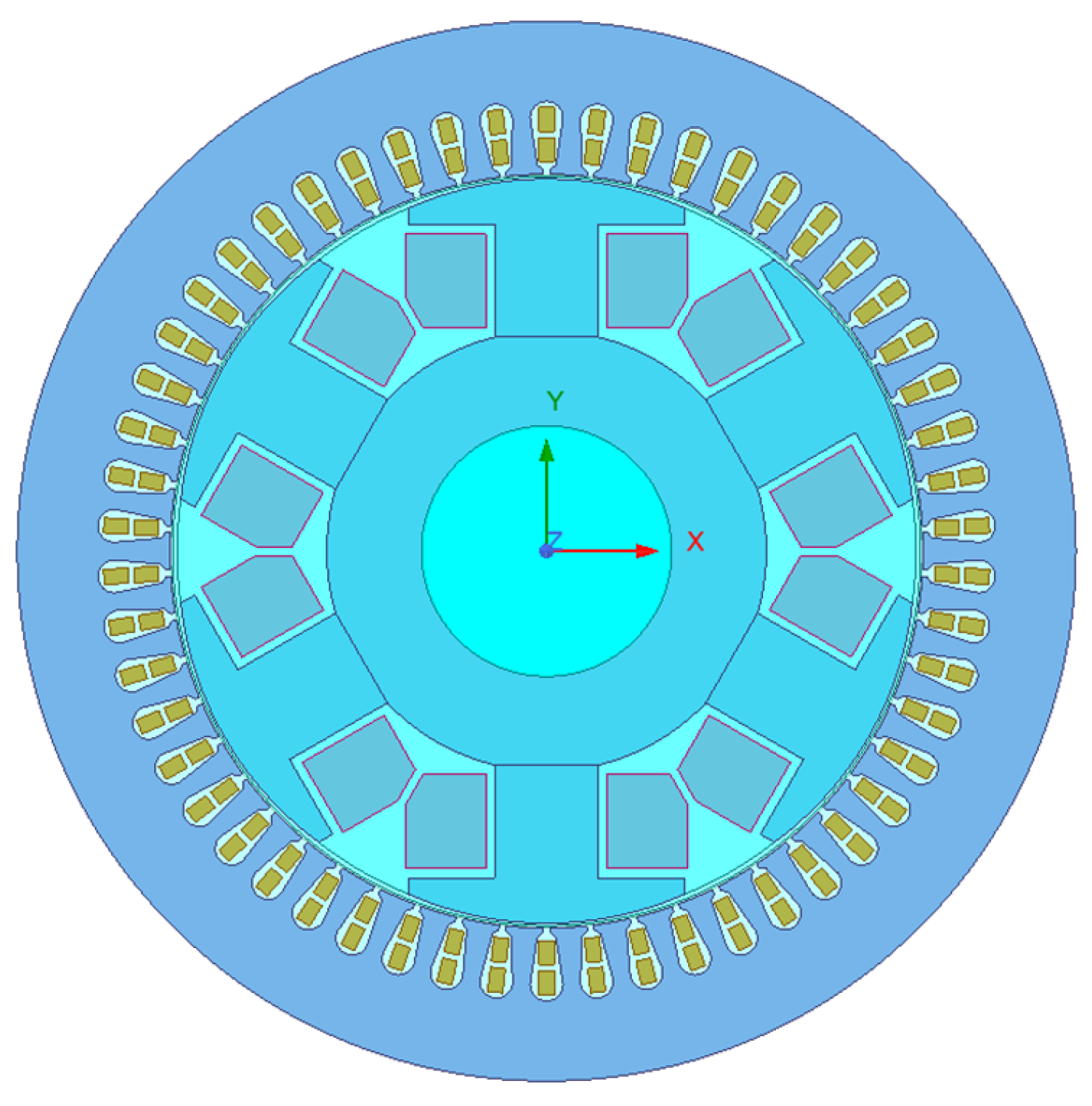
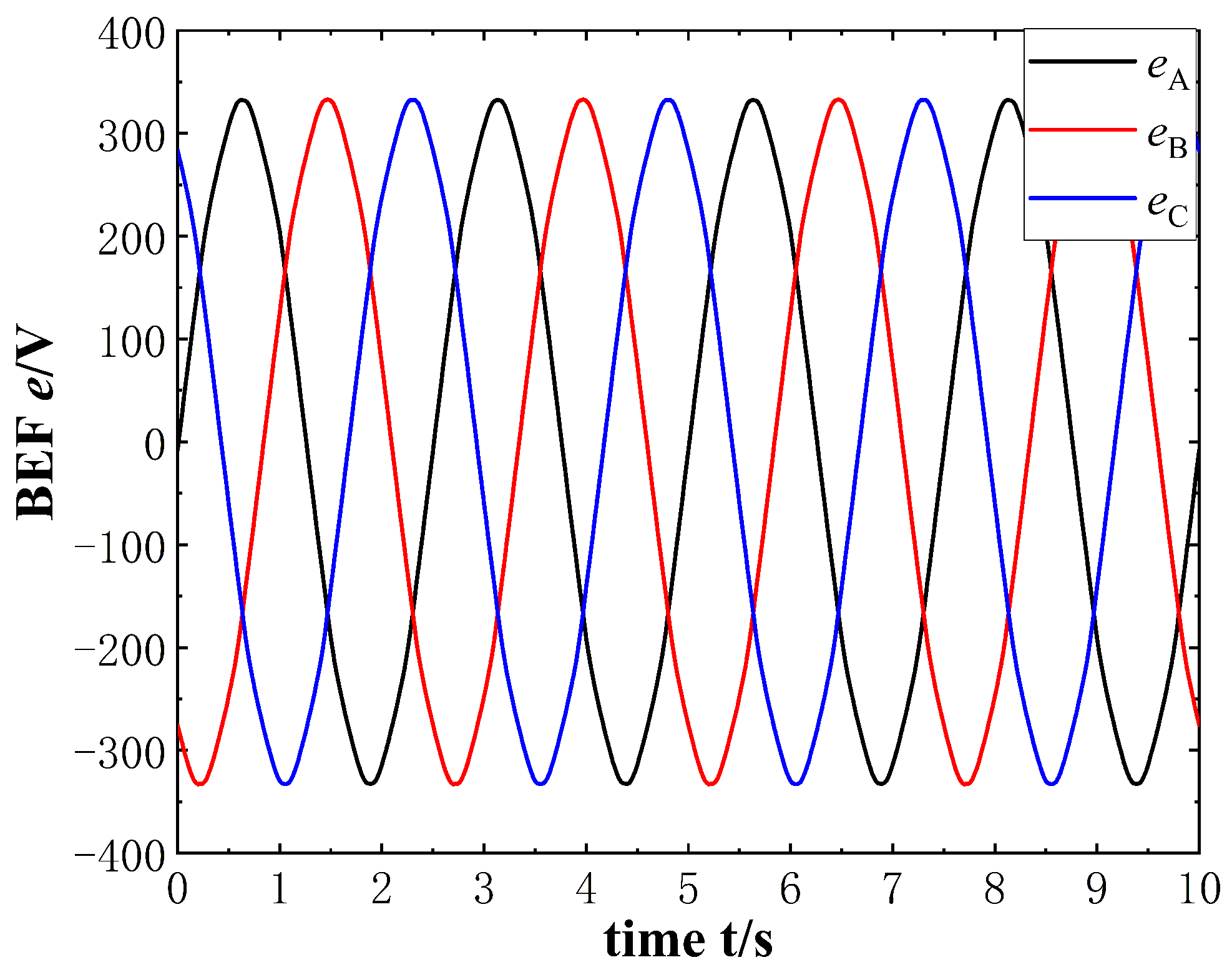
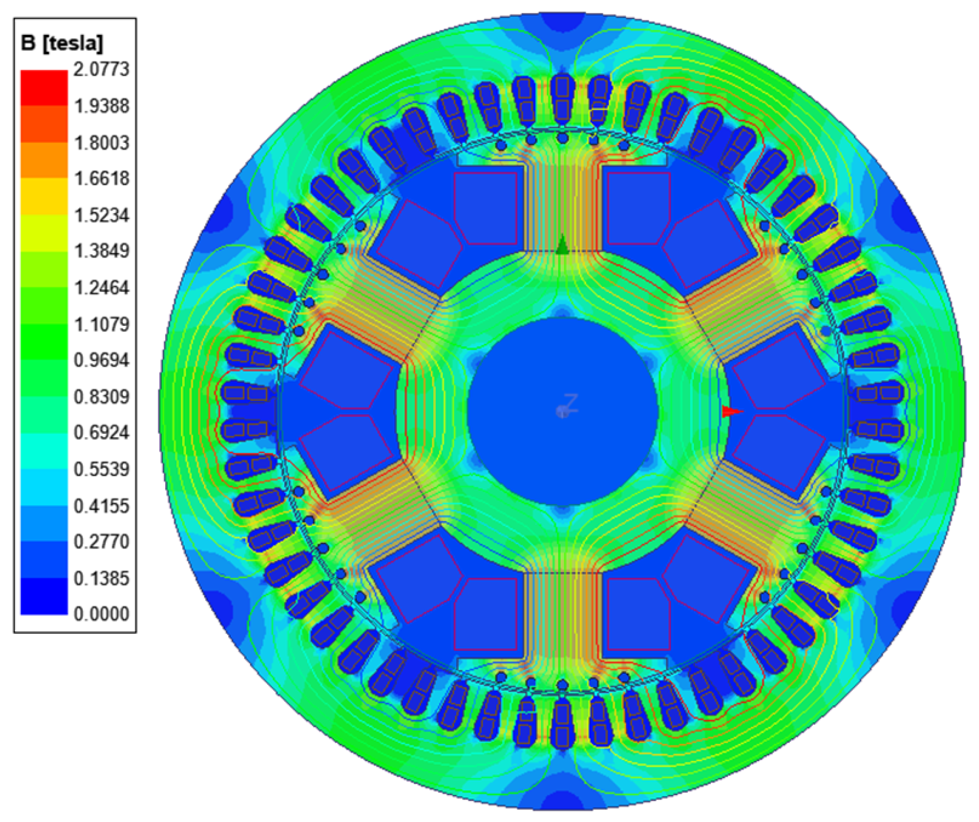
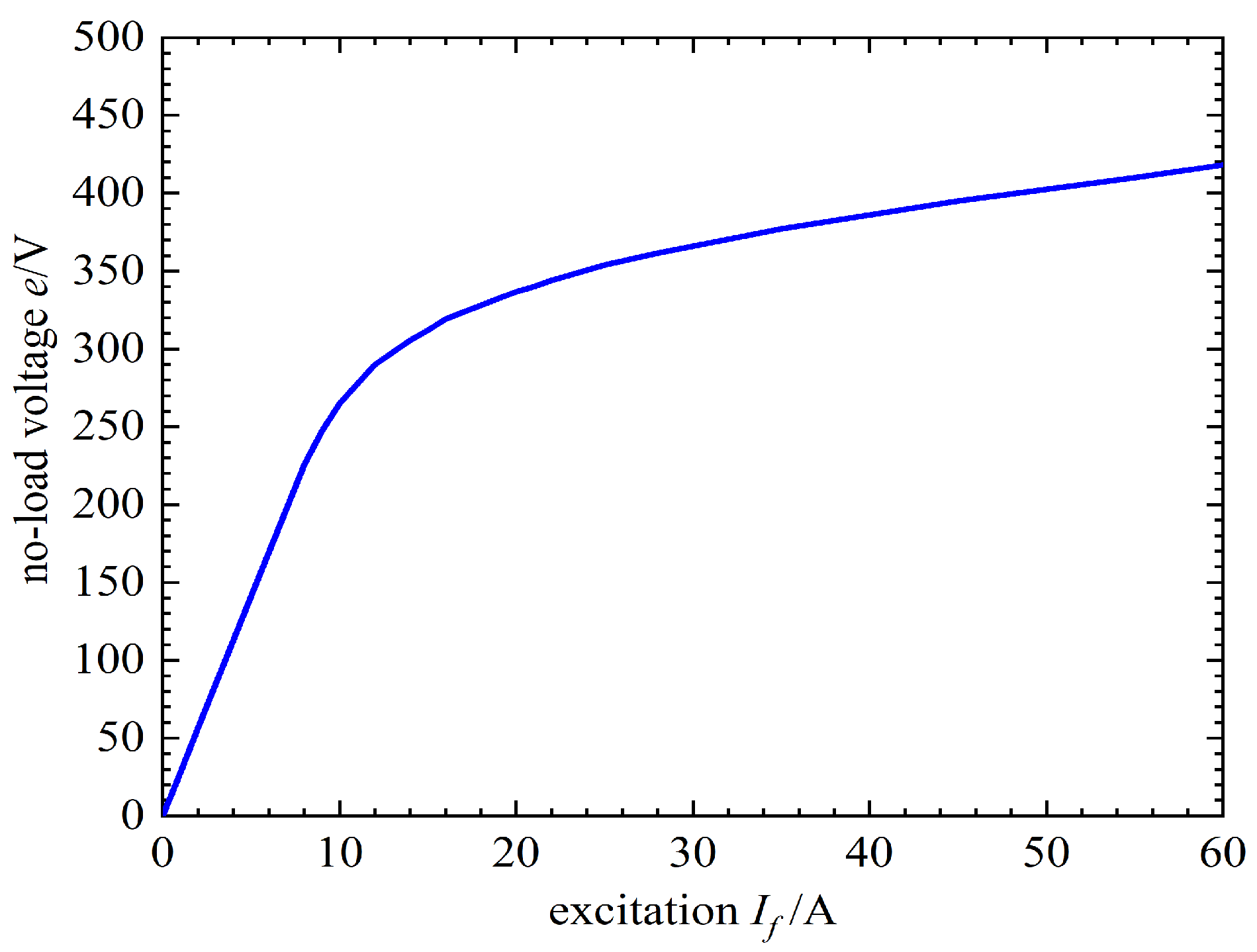
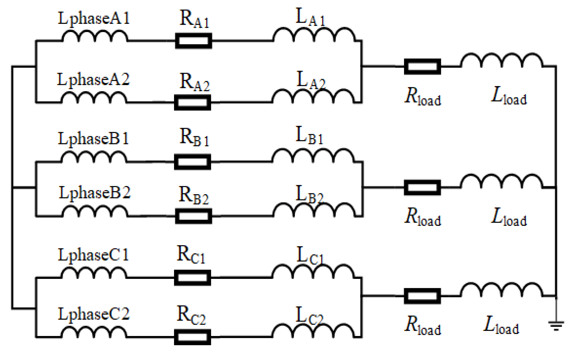
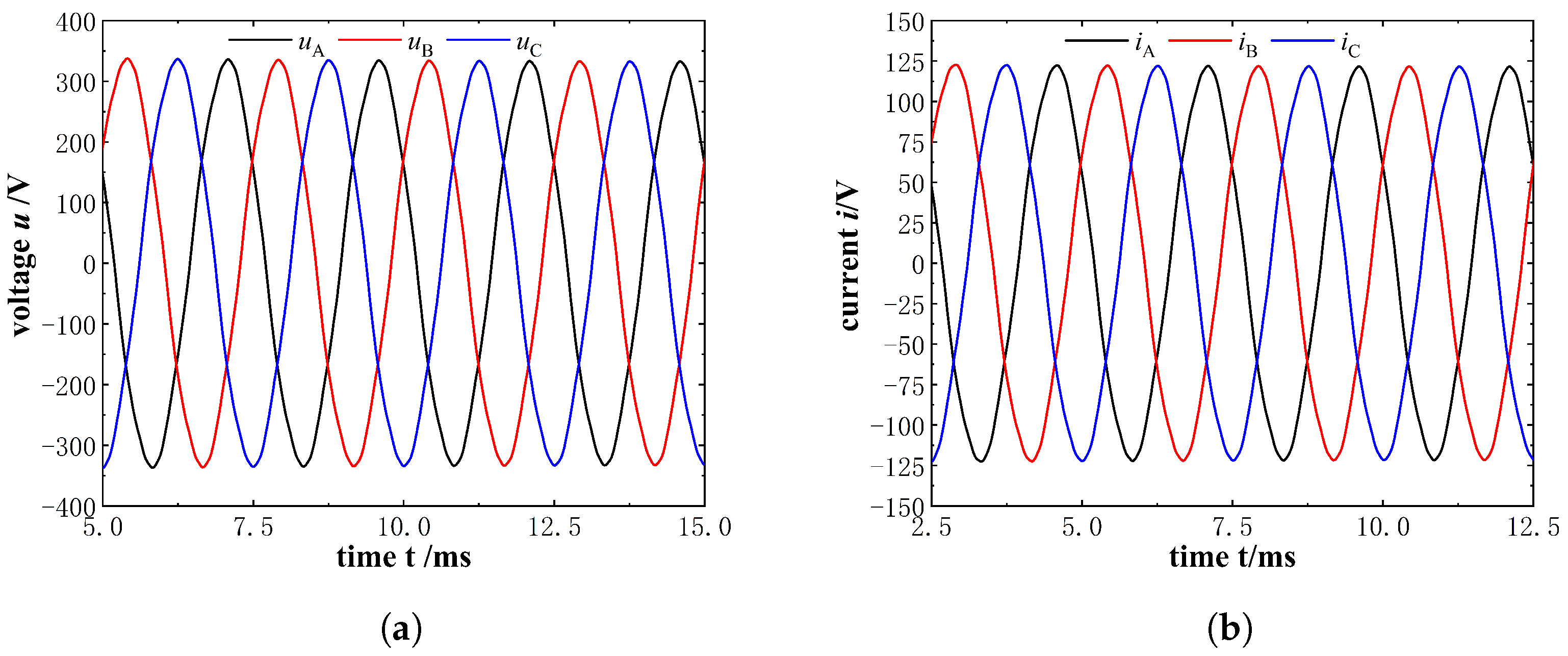
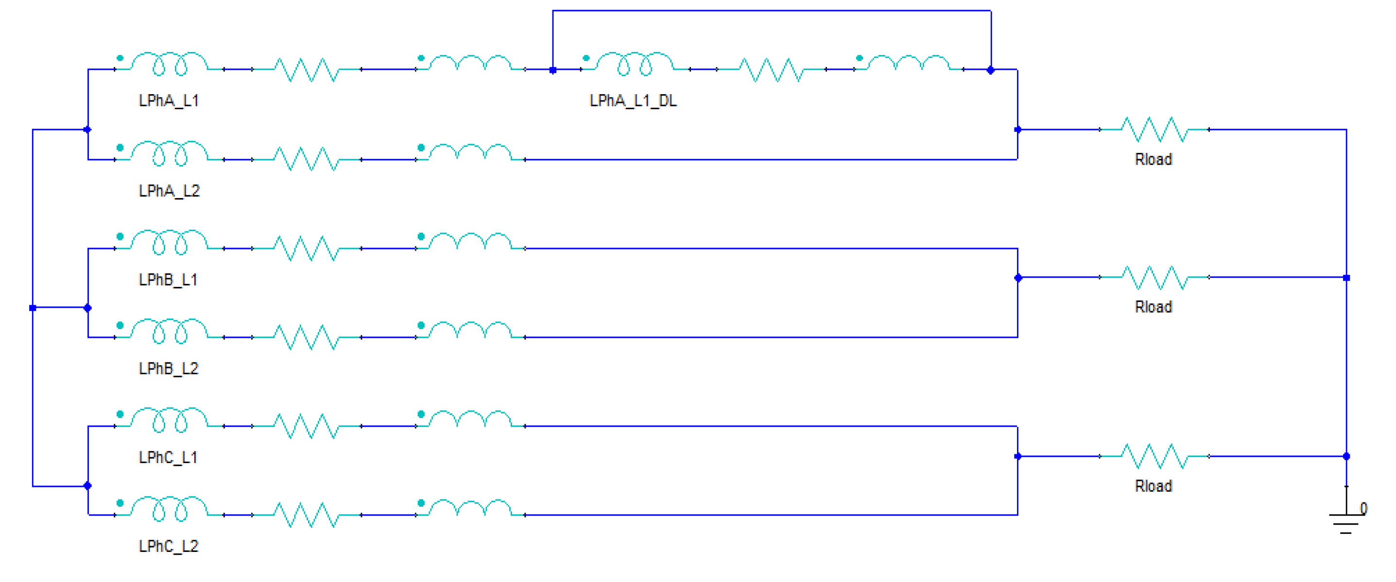
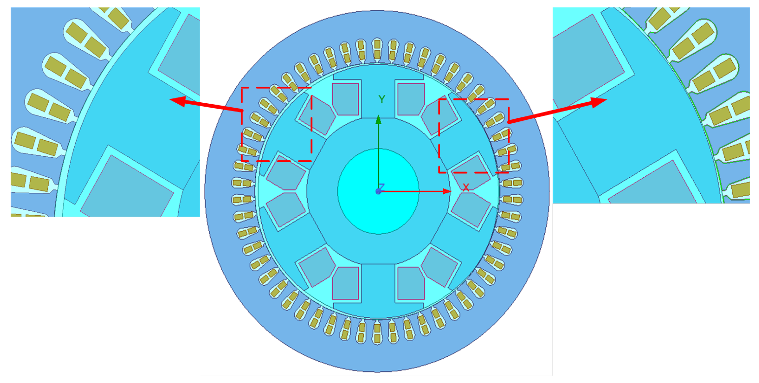
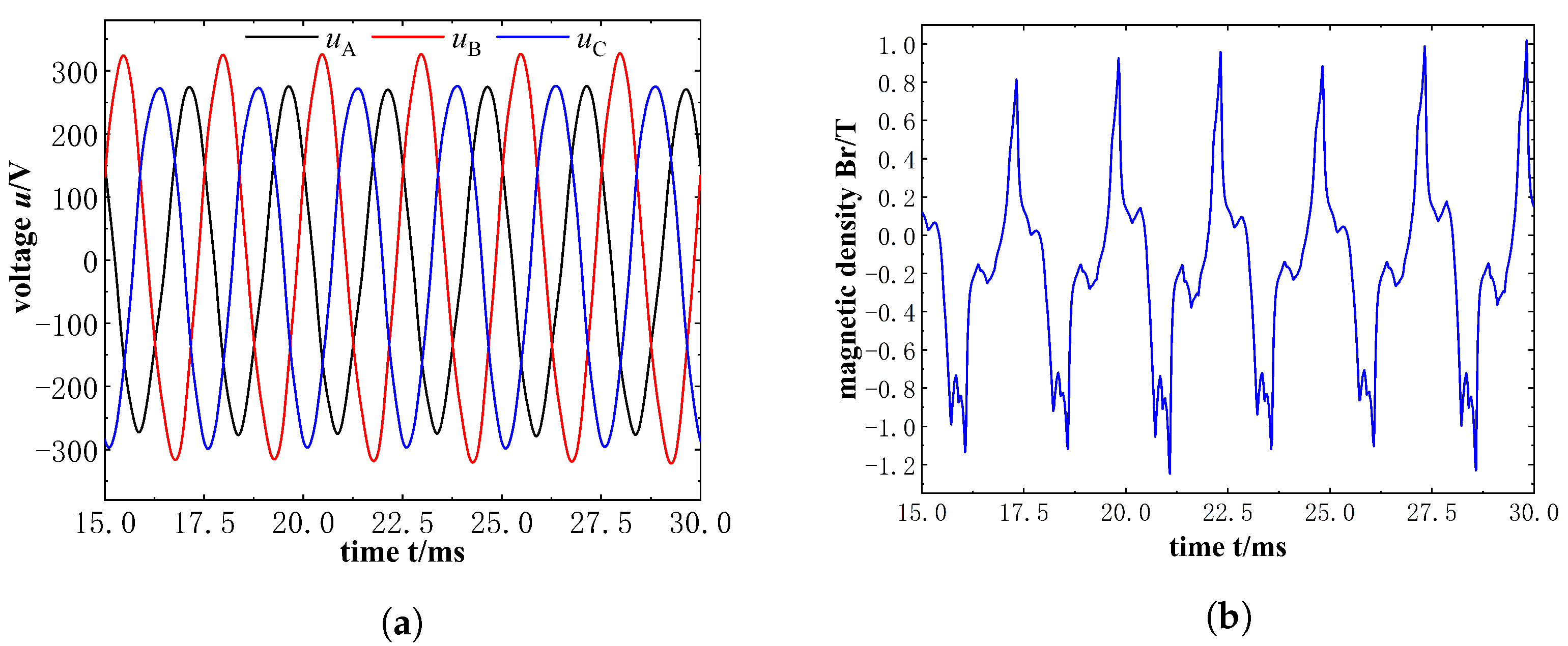
2.2. FEM Model of the Aviation Generator
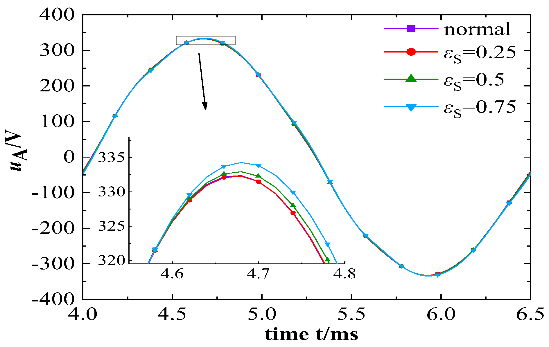
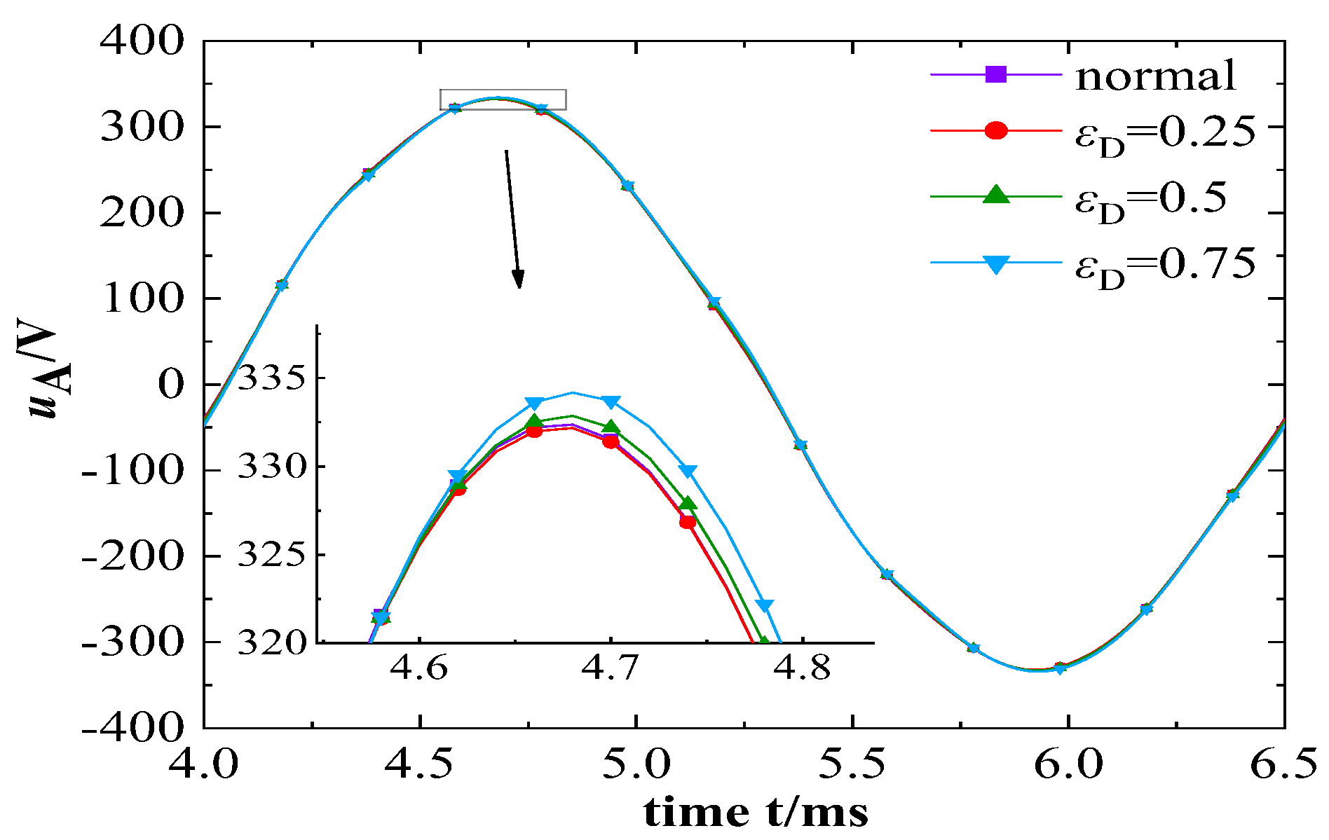
2.3. Model of Composite Faults
3. Feature Extraction and Fault Diagnosis Algorithm
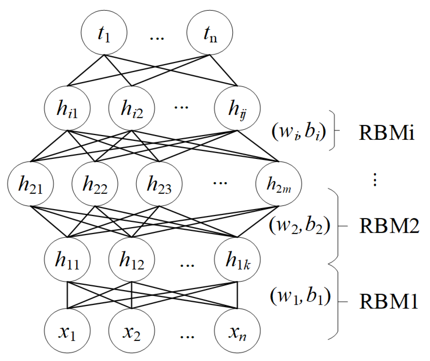
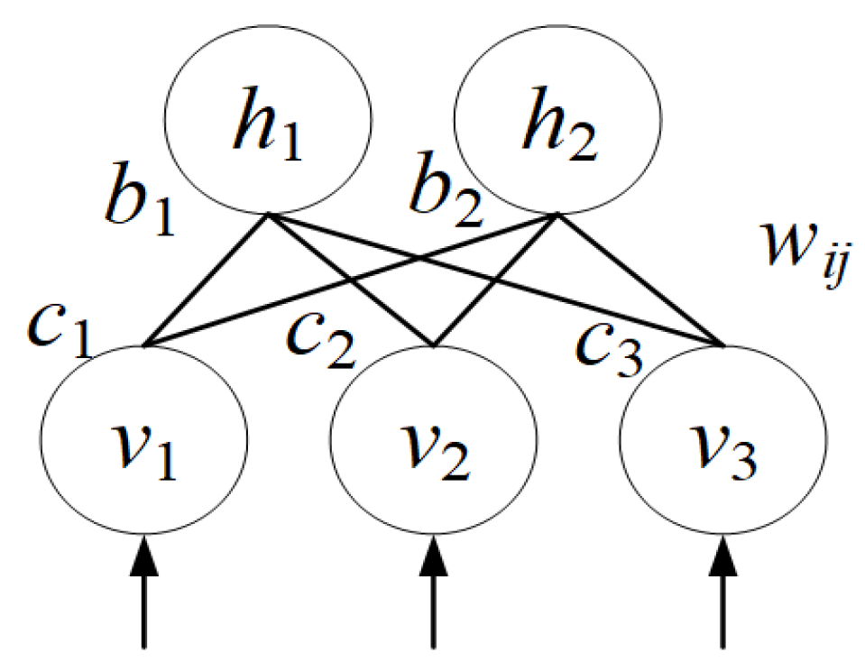
3.1. DBN
3.2. ELM
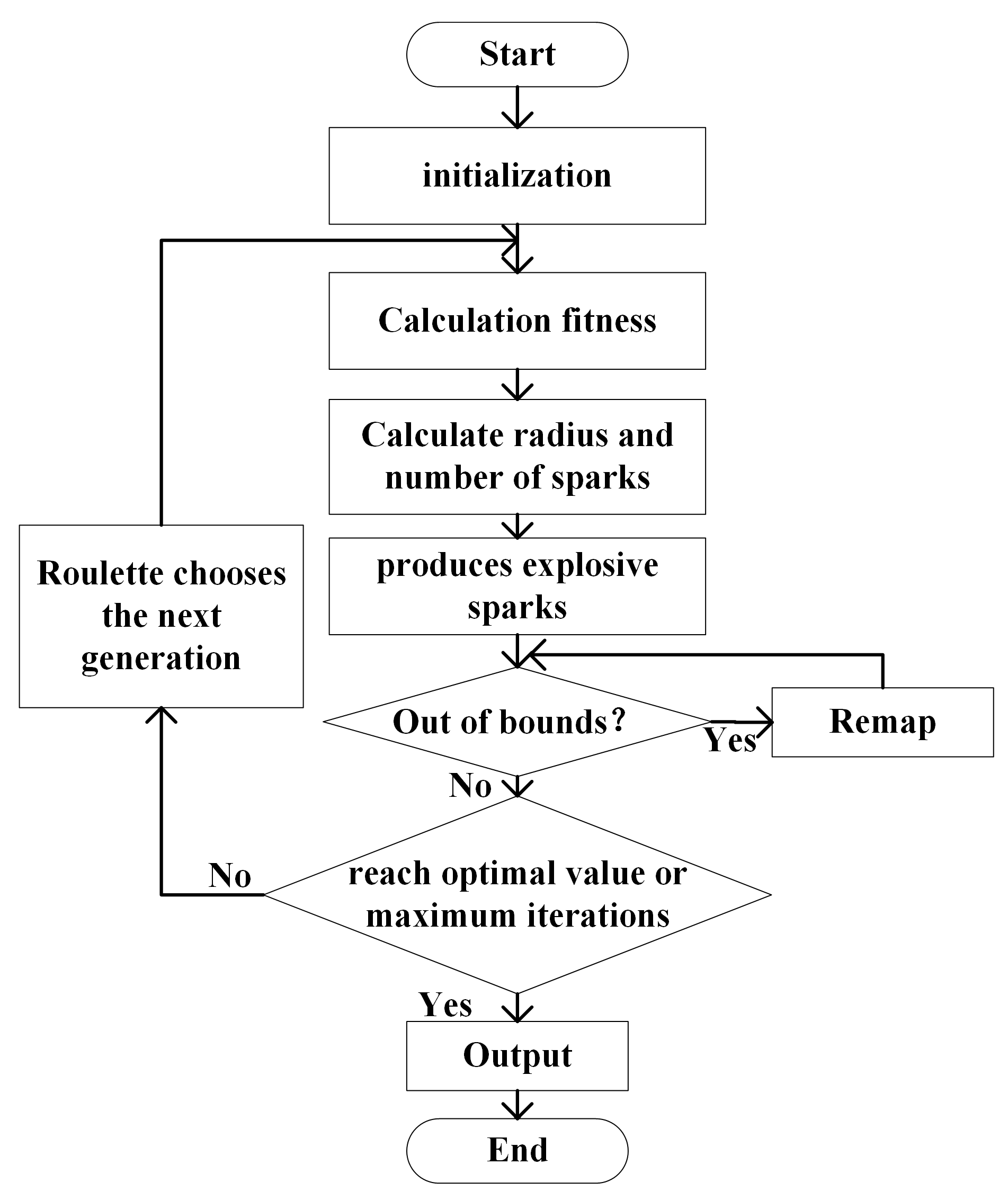
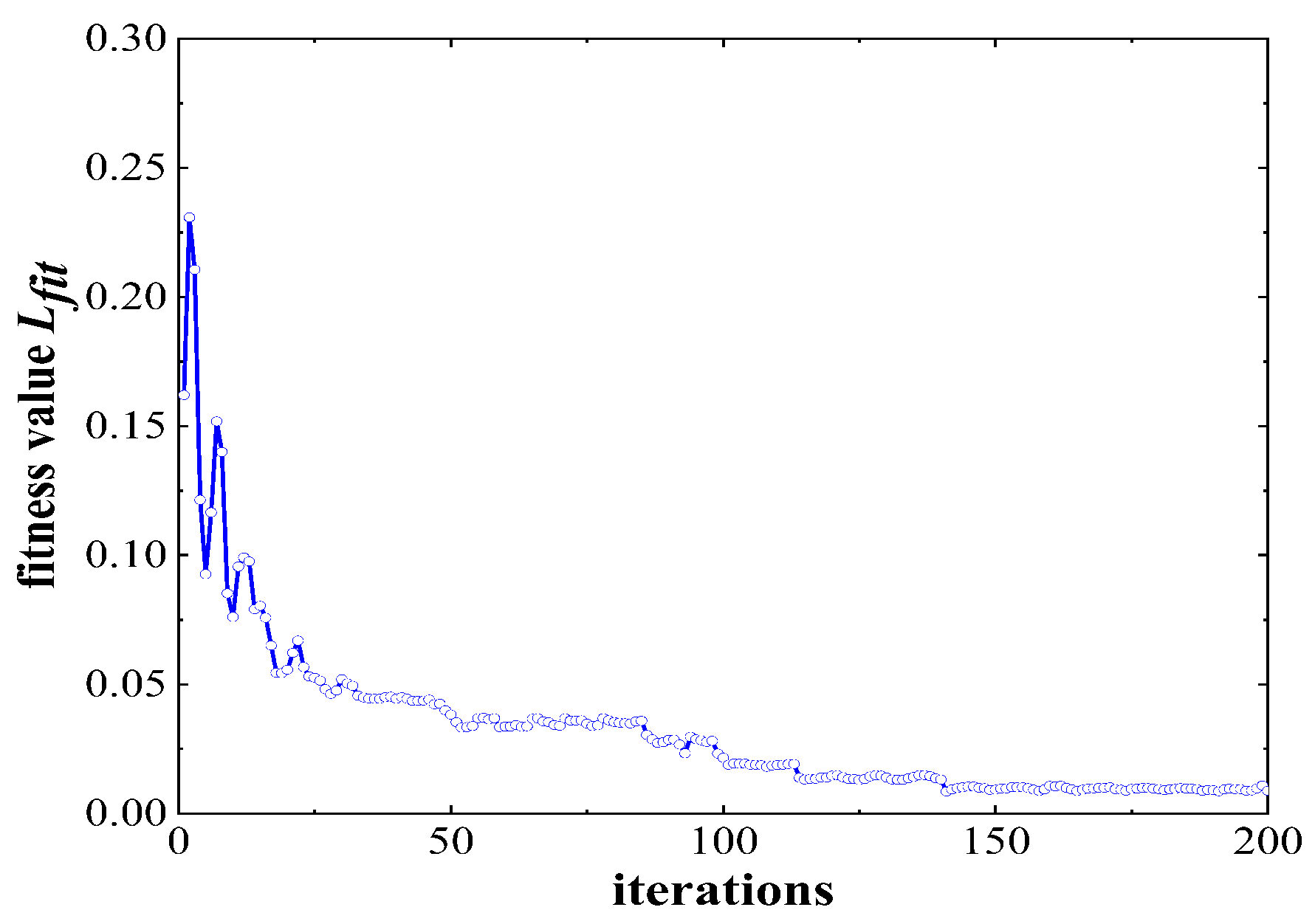
3.3. EnFWA
3.4. Comparisons of Different Diagnostic Models
- (1)
- FFT + EnFWA + DBN: Preliminary feature extraction was carried out on the output voltage and current data with fast Fourier transform (FFT). Features of the first 20 frequency components were used for training and diagnosing with the same network structure.
- (2)
- PSO + DBN: PSO algorithm was used to train and optimize the DBN. The number of particles is 50, the acceleration coefficient = = 0.5, and the inertia weight decreased from 0.9 to 0.4.
- (3)
- SDAE + SVM: the stacked denoising autoencoder (SDAE) was used for feature extraction of the fault data and support vector machine (SVM) was used for fault diagnosis. The structure of SDAE hidden layer is [150−75−20], sparse coefficient is 0.15, penalty weight is 3, SVM penalty parameter C = 49.43, and kernel parameter g = 100.
- (4)
- LSTM + Softmax: The long short-term memory (LSTM) was used to extract fault data features and the softmax was used for fault diagnosis. Set the number of LSTM hidden layer neurons as [14−14], the learning rate as 0.01, and the length of sliding window as 10.
4. Data Collection and Diagnosis
5. Conclusions
Author Contributions
Funding
Data Availability Statement
Conflicts of Interest
Abbreviations
| FWA | Fireworks Algorithm |
| EnFWA | Enhanced Fireworks Algorithm |
| ELM | Extreme Learning Machine |
| DBN | Deep Belief Network |
| DC | Direct Current |
| RBM | Restricted Boltzmann Machine |
| FFT | Fast Fourier Transform |
| PSO | Particle Swarm Optimization |
| FEM | Finite Element Method |
| BEF | Back Electromotive Force |
| RMS | Root Mean Square |
| SDAE | Stacked Denoising Auto Encoder |
| SVM | Support Vector Machine |
| LSTM | Long Short Term Memory |
References
- IEEE.Std. IEEE Recommended Practice for the Design of Reliable Industrial and Commercial Power Systems—Redline. In IEEE Std 493-2007 (Revision of IEEE Std 493-1997)—Redline; IEEE: Piscataway, NJ, USA, 2007; pp. 1–426. [Google Scholar]
- Sadeghi, I.; Ehya, H.; Faiz, J. Analytic method for eccentricity fault diagnosis in salient-pole synchronous generators. In Proceedings of the 2017 International Conference on Optimization of Electrical and Electronic Equipment (OPTIM) & 2017 Intl Aegean Conference on Electrical Machines and Power Electronics (ACEMP), Brasov, Romania, 25–27 May 2017; pp. 261–267. [Google Scholar] [CrossRef]
- He, Y.L.; Zhang, W.; Xu, M.X.; Tao, W.Q.; Liu, H.L.; Dou, L.J.; Wan, S.T.; Li, J.Q.; Gerada, D. Rotor loss and temperature variation under single and combined faults composed of static air-gap eccentricity and rotor inter-turn short circuit in synchronous generators. IET Electr. Power Appl. 2021, 15, 1529–1546. [Google Scholar] [CrossRef]
- Ehya, H.; Nysveen, A.; Nilssen, R.; Liu, Y. Static and dynamic eccentricity fault diagnosis of large salient pole synchronous generators by means of external magnetic field. IET Electr. Power Appl. 2021, 15, 890–902. [Google Scholar] [CrossRef]
- Zhang, J.; Xiong, X.; Zhou, Y.; Wang, K. Rotor Eccentric Diagnosis of High-Voltage Motor in Nuclear CRF Pump Using Vibration Signals. In Proceedings of the 2021 7th International Conference on Condition Monitoring of Machinery in Non-Stationary Operations (CMMNO), Guangzhou, China, 11–13 June 2021; pp. 282–286. [Google Scholar] [CrossRef]
- Shuting, W.; Yuling, H. Analysis on stator circulating current characteristics of turbo-generator under eccentric faults. In Proceedings of the 2009 IEEE 6th International Power Electronics and Motion Control Conference, Wuhan, China, 17–20 May 2009; pp. 2062–2067. [Google Scholar] [CrossRef]
- Swana, E.F.; Doorsamy, W. Investigation of Combined Electrical Modalities for Fault Diagnosis on a Wound-Rotor Induction Generator. IEEE Access 2019, 7, 32333–32342. [Google Scholar] [CrossRef]
- Tamilselvan, P.; Wang, P. Failure diagnosis using deep belief learning based health state classification. Reliab. Eng. Syst. Saf. 2013, 115, 124–135. [Google Scholar] [CrossRef]
- Yang, L.; Wang, J.; Zhang, G.; Li, X.; Fu, H. An Adaptive Fault Diagnosis System Framework for Aircraft Based on Man-in-loop. In Proceedings of the 2019 IEEE International Conference on Prognostics and Health Management (ICPHM), San Francisco, CA, USA, 17–20 June 2019; pp. 1–4. [Google Scholar] [CrossRef]
- Tran, V.T.; AlThobiani, F.; Ball, A. An approach to fault diagnosis of reciprocating compressor valves using Teager-Kaiser energy operator and deep belief networks. Expert Syst. Appl. 2014, 41, 4113–4122. [Google Scholar] [CrossRef]
- Tran, V.T.; AlThobiani, F.; Tinga, T.; Ball, A.; Niu, G. Single and combined fault diagnosis of reciprocating compressor valves using a hybrid deep belief network. Proc. Inst. Mech. Eng. Part C-J. Mech. Eng. Sci. 2018, 232, 3767–3780. [Google Scholar] [CrossRef]
- Luo, H.; He, C.; Zhou, J.; Zhang, L. Rolling Bearing Sub-Health Recognition via Extreme Learning Machine Based on Deep B Network Optimized by Improved Fireworks. IEEE Access 2021, 9, 42013–42026. [Google Scholar] [CrossRef]
- Zheng, S.; Li, J.; Janecek, A.; Tan, Y. A Cooperative Framework for Fireworks Algorithm. IEEE-ACM Trans. Comput. Biol. Bioinform. 2017, 14, 27–41. [Google Scholar] [CrossRef] [PubMed]
- Gohari, M.; Eydi, A.M. Modelling of shaft unbalance: Modelling a multi discs rotor using K-Nearest Neighbor and Decision Tree Algorithms. Measurement 2020, 151, 107253. [Google Scholar] [CrossRef]
- Luo, S.; Cheng, J.; Zeng, M.; Yang, Y. An intelligent fault diagnosis model for rotating machinery based on multi-scale higher order singular spectrum analysis and GA-VPMCD. Measurement 2016, 87, 38–50. [Google Scholar] [CrossRef]
- Shao, H.; Jiang, H.; Zhang, X.; Niu, M. Rolling bearing fault diagnosis using an optimization deep belief network. Meas. Sci. Technol. 2015, 26, 115002. [Google Scholar] [CrossRef]
- Wu, S.; Zheng, L.; Hu, W.; Yu, R.; Liu, B. Improved Deep Belief Network and Model Interpretation Method for Power System Transient Stability Assessment. J. Mod. Power Syst. Clean Energy 2020, 8, 27–37. [Google Scholar] [CrossRef]
- Shan, H.; Sun, Y.; Zhang, W.; Kudreyko, A.; Ren, L. Reliability Analysis of Power Distribution Network Based on PSO-DBN. IEEE Access 2020, 8, 224884–224894. [Google Scholar] [CrossRef]
- Zhang, C.; He, Y.; Yuan, L.; Xiang, S. Analog Circuit Incipient Fault Diagnosis Method Using DBN Based Features Extraction. IEEE Access 2018, 6, 23053–23064. [Google Scholar] [CrossRef]
- Mackerle, J. FEM and BEM analysis and modelling of residual stresses—A bibliography (1998–1999). Finite Elem. Anal. Des. 2001, 37, 253–262. [Google Scholar] [CrossRef]


| Stator | Rotor | ||
|---|---|---|---|
| Outer diameter/mm | 230 | Outer diameter/mm | 158 |
| inner diameter/mm | 160 | shaft diameter/mm | 53.2 |
| the number of slot | 54 | core length/mm | 103 |
| core length/mm | 103 | pole pairs | 3 |
| material | DW315_50 | material | M27_24G |
| connection of winding | Y | turns each pole | 50 |
| winding pitch | 6 | width of pole shoe/mm | 58.6 |
| branch | 2 | height of pole shoe/mm | 9.6 |
| conductors per slot | 10 | pole-core width/mm | 22 |
| width of air gap/mm | 1 | pole-core height/mm | 24 |
| wire size/mm | 1.219 | polar arc coefficient | 0.72 |
| resistance of each phase/ | 0.126 | resistance of field winding/ | 0.44 |
| Algorithm | Single Eccentricity Fault | Composite Fault | ||
|---|---|---|---|---|
| Accuracy/% | Duration/s | Accuracy/% | Duration/s | |
| FFT + EnFWA + DBN | 89.882 | 8.46 | 86.718 | 6.19 |
| PSO + DBN | 95.622 | 11.04 | 94.371 | 9.88 |
| SDAE + SVM | 92.677 | 20.81 | 92.445 | 18.27 |
| LSTM + Softmax | 93.493 | 12.06 | 93.986 | 10.62 |
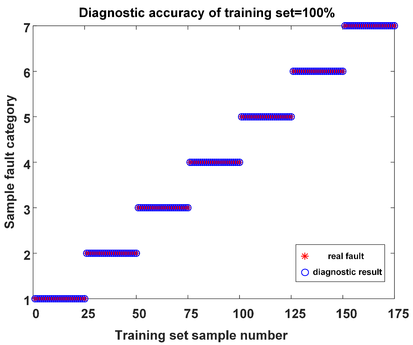
| Algorithm of this paper | 99.144 | 9.34 | 97.857 | 7.08 |
| Fault Category | Type | Training Data | Test Data |
|---|---|---|---|
| 1 | Normal | 7.5 × 10⁵ | 1.5 × 10⁵ |
| 2 | 1/9 A phase short-out + 5% Dynamic eccentricity | 7.5 × 10⁵ | 1.5 × 10⁵ |
| 3 | 1/9 A phase short-out + 5% Static eccentricity | 7.5 × 10⁵ | 1.5 × 10⁵ |
| 4 | 2/9 A phase short-out + 15% Dynamic eccentricity | 7.5 × 10⁵ | 1.5 × 10⁵ |
| 5 | 2/9 A phase short-out + 15% Static eccentricity | 7.5 × 10⁵ | 1.5 × 10⁵ |
| 6 | 3/9 A phase short-out + 25% Dynamic eccentricity | 7.5 × 10⁵ | 1.5 × 10⁵ |
| 7 | 3/9 A phase short-out + 25% Static eccentricity | 7.5 × 10⁵ | 1.5 × 10⁵ |
Disclaimer/Publisher’s Note: The statements, opinions and data contained in all publications are solely those of the individual author(s) and contributor(s) and not of MDPI and/or the editor(s). MDPI and/or the editor(s) disclaim responsibility for any injury to people or property resulting from any ideas, methods, instructions or products referred to in the content. |
© 2023 by the authors. Licensee MDPI, Basel, Switzerland. This article is an open access article distributed under the terms and conditions of the Creative Commons Attribution (CC BY) license (https://creativecommons.org/licenses/by/4.0/).
Share and Cite
Yang, Z.; Bao, X.; Zhou, Q.; Yang, J. Composite Fault Diagnosis of Aviation Generator Based on EnFWA-DBN. Processes 2023, 11, 1577. https://doi.org/10.3390/pr11051577
Yang Z, Bao X, Zhou Q, Yang J. Composite Fault Diagnosis of Aviation Generator Based on EnFWA-DBN. Processes. 2023; 11(5):1577. https://doi.org/10.3390/pr11051577
Chicago/Turabian StyleYang, Zhangang, Xingwang Bao, Qingyu Zhou, and Juan Yang. 2023. "Composite Fault Diagnosis of Aviation Generator Based on EnFWA-DBN" Processes 11, no. 5: 1577. https://doi.org/10.3390/pr11051577