Article

Modification of Meso-Micromixing Interaction Reaction Model in Continuous Reactors

School of Chemical Engineering and Technology, Tianjin University, Tianjin 300350, China
*
Author to whom correspondence should be addressed.
These authors contributed equally to this work.
Processes 2023, 11(5), 1576; https://doi.org/10.3390/pr11051576
Submission received: 25 April 2023 / Revised: 15 May 2023 / Accepted: 16 May 2023 / Published: 22 May 2023
(This article belongs to the Special Issue CFD Applications in Energy Engineering Research and Simulation)

Abstract

:
The yields of chemical reactions are highly dependent on the mixing pattern between reactants. Herein, we report the modification of a meso-micromixing interaction reaction model which is applied in batch reactors by leveraging the flow characteristics in the continuous reactors. Both experimental and model-predicted yields were compared using the classical Villermaux–Dushman method in a self-designed split and recombination reactor. This modified model significantly reduced the error in predicted product yields from approximately 15% to within 3%, compared to a model containing the micromixing term only. The effects of flow rates and reactor structure parameters on mixing performance were analyzed. We found that increasing flow rates and the degree of twist in the mixing element’s grooves, as well as decreasing the cross-sectional area of grooves, improved mixing performance. The optimization of reactor flow rates and structural parameters was achieved by combining Gaussian process regression and Bayesian optimization with the modified model. This approach provided higher target product yields for consecutive reactions, while simultaneously achieving a lower pressure drop in the reactor. Corresponding combinations of reactor parameters were also identified during this process. Our modified model-based optimization methodology can be applied to a diversity of reactors, serving as a reference for the selection of their structure and operational parameters.

Graphical Abstract

1. Introduction

Consecutive reactions are extensively employed in the chemical process industry (CPI), such as in the synthesis of pharmaceuticals and high-performance polymers [1,2,3]. Studying consecutive reaction yields is crucial for assessing the reactions’ performance and designing synthetic routes [4]. In cases where the reaction rate is less than or equal to the mixing rate, mixing within the reactor governs the contact pattern of the various species involved, thereby influencing their distributions. Consider the following consecutive reactions:
A + B k 1 R A + R k 2 S
These reactions are second-order, where the yield of the desired product S is:
Y S = 2 c S c A 0
Proper control of mixing quality is essential to maximize the yield of the target product S when k 1 > k 2 , and has been extensively studied [5,6,7,8,9,10]. Christy et al. investigated the reaction between 1,2 diphenyl ethane (B) and NO2BF4 (A) [8]. They found that the yield of the polynitro product (S) decreased from 78% to 54% upon increasing the stirring intensity then improving mixing uniformity. This decrease in yield can be attributed to different distribution states of the nitrifying agent (A) in the reactor [11]. Enhancing mixing homogeneity resulted in a uniform distribution of A and a rapid decrease in its local concentration within the reactor after the formation of R. This can lead to the continuous accumulation of R, less subsequent reactions taking place, and, finally, a decrease in Y S . However, these studies merely qualitatively evaluated the effect of mixing performance on consecutive reaction yields without analyzing yields governed by mixing processes quantitatively.
The quantitative relationship between mixing and yields can be described using a reaction model containing parameters characterizing mesomixing and micromixing. Baldyga and Bourne proposed a model in terms of the influence of meso- and micromixing on reactions and applied it to a semi-batch reactor with an extremely high flow ratio of two mixing streams [12]. The simulation results had a good prediction accuracy with a yield error of ±2% compared to experimentally measured yields. Samant et al. studied consecutive reactions in a stirred batch reactor based on this model [13]. They found that structural parameters, such as the stirring paddle shape and the number of feed points, had significant effects on mixing rate-limited steps and reaction yields. Then they provided empirical correlations of mixing characteristic times at each scale controlled by these parameters to guide the reactor design.
Continuous reactors have many parameters that can significantly affect the internal fluid flow and mixing pattern, which, in turn, affect the yield of consecutive reactions [14,15,16,17,18]. Baldyga and Bourne used the aforementioned model to forecast the yield in a Kenics tubular reactor with a flow ratio of 3000:1 [12]. However, the yield was mainly influenced by the mixing pattern of the stream with the extremely low flow rate, which does not hold true for two streams with comparable flow rates in tubular reactors. Thus, the model requires modification based on the flow and mixing characteristics in such cases. Nevertheless, no model modification work has been conducted for meso-micromixing interaction reaction models in tubular reactors, which could ascertain the ambient fluid concentration of the reagents and the volume change of the fluid due to mixing.
The structural parameters of tubular reactors not only influence the mixing pattern and target product yield of reactions but are also closely related to the pressure drop in reactors. Maximizing the target product yield while keeping the pressure drop within a reasonable range is a valuable pursuit of study [19]. However, optimizing numerous parameters of reactors based on the reaction model can be computationally challenging [20]. Multidimensional regression and optimization required for this process are difficult to carry out. Gaussian process regression combined with Bayesian optimization can provide a general optimal solution for nonlinear optimization problems with fewer iterations and higher calculation speed [21,22,23]. Zuhal et al. [24] and Seongeon Park [25] employed CFD to conduct a series of Bayesian optimization designs to optimize the structure of the airfoil and stirred batch reactor based on minimum pressure drop criteria. However, there are currently no relevant studies on the structural design of continuous reactors that link reaction models with optimization methods to evaluate the relationship between target product yields and the pressure drop in reactors.
In this study, we analyze the flow characteristics and mixing pattern in continuous reactors and modify the meso-micromixing interaction reaction model which had been used in batch conditions in previous work. We use the Villermaux–Dushman method in a self-fabricated split and recombination reactor to verify the model’s accuracy by comparing the results obtained by experiments with the model. We analyze the changes in mixing performance due to parameter variations from a flow field perspective. We use this modified model combined with Gaussian process regression and Bayesian optimization to obtain higher yields of target products in consecutive reactions while maintaining a lower pressure drop in the reactor. Such a design method can be applied to the optimization of various types of reactors.

2. Modified Meso-Micromixing Interaction Reaction Model

2.1. Initial Mixing-Related Reaction Model

According to Baldyga and Bourne’s theory [12], a meso- and micromixing interaction reaction model can be characterized by the following equation:
d c i d t = E ( 1 X B X u ) ( c i c i ) + r i
The symbols in this equation are defined as follows: The rate of engulfment, E , describes the micromixing of fluid elements, which will be explained in detail in Section 3.4. X u represents a fraction of the fluid volume. This part of the fluid contains partially segregated fluid as islands embedded in a sea, where the reagents are coarsely mixed and concentration fluctuations still exist. X u can be derived by statistical method:
The variance of composition of the
X u = X 0 X 0 + ( 1 X 0 ) exp ( t t d )
The initial volume fraction in the reactor where the reagents are present is X 0 . For tubular reactors, X 0 can be considered as the ratio of the initial flow rates. As X u tends to 1, it signifies that the reagents spread everywhere from the mesomixing perspective, although without being completely micromixed.
X B refers to the volume of micromixed fluid relative to the whole fluid. According to the engulfment model, the rate of engulfment from E model is:
d X B d t = E X B ( 1 X B X u )
This equation describes the micromixing pattern when mesomixing is incomplete. Initially the islands, whose initial volume fraction is X 0 , only consist of pure B-rich feed, so that the initial value of X B is also X 0 . As the flow enters the reactor, eddy breakup increases X u , which initiates micromixing.

2.2. Comparison of Batch and Continuous Conditions

In batch reactors, the limited reagents are added dropwise. The chemical reaction occurs only in the droplets. The ambient fluid concentration 〈 c i 〉 outside the micromixing region can be assumed to be a constant concentration of excess fluid in the reactor. Additionally, when the flow rate in one of these streams is extremely low, the volume of fluid that has been fully micromixed will be present only in the other excessive stream.
In the case of two comparable flow rates in the continuous reactors, chemical reactions can occur in both streams after achieving micromixing. This implies that each stream contains a significant concentration of reagents and products, as was shown in Figure 1. As a result, the ambient fluid concentration 〈 c i 〉 is no longer a changeless concentration, which is the case in batch reactors. Furthermore, when the flow rates are comparable, both flows experience reciprocal engulfment effects and micromixing. Consequently, the volume of fluid that is completely micromixed in both streams changes (in Figure 1, the total volume of each stream is V A + Δ V A or V B + Δ V B ), which ultimately impacts the concentration of species in each stream.

2.3. Model Modification

We have modified the model after accounting for the differences between the above two conditions.
Firstly, since both streams, 1 and 2, exhibit self-engulfment behavior and undergo chemical reactions, we considered the ambient species’ concentration outside the micromixing region of stream 1 as that of the corresponding species in stream 2, and vice versa. In other words, these two streams are treated as reciprocal environmental fluids, as was shown in Figure 1.
Secondly, since the change in fluid volume resulting from the mesomixing and micromixing in these two streams is not negligible, we took stream 1 as the reference and switched from the concentration change due to the volume change of stream 2 to the volume-based concentration of stream 1. To describe this behavior, we introduced a fluid volume change rate φ B , which essentially represents the fluid volume change induced by mixing at the mesoscopic and microscopic scales. This rate can be calculated using the following integrated equation:
φ B = e t + ( 1 1 e Q t ) Q
Here, Q is the ratio of the micromixing characterized time and the mesomixing characterized time.
Based on these, the model can be modified as (taking concentrated reagent A in stream 1 for instance):
d c A 1 d t = E ( 1 X B 1 X u A ) ( c A 2 c A 1 ) + r A
d c A 2 d t = [ E ( 1 X B 2 X u A ) ( c A 1 c A 2 ) + r A ] V t o t a l V A ( V A + V B ) φ B ( V t o t a l V t o t a l V A ( V A + V B ) φ B )
where V t o t a l V A ( V A + V B ) is the inlet flow rate of stream 1.
By analogy, each species is governed by two ordinary differential equations that control its concentration in each of these two fluid environments (stream 1 and stream 2). In Equation (7), the subscript 1 represents the fluid that has undergone micromixing, while the subscript 2 represents the ambient fluid surrounding stream 1. For Equation (8), the opposite is true of what was explained above.

3. Methods and Materials

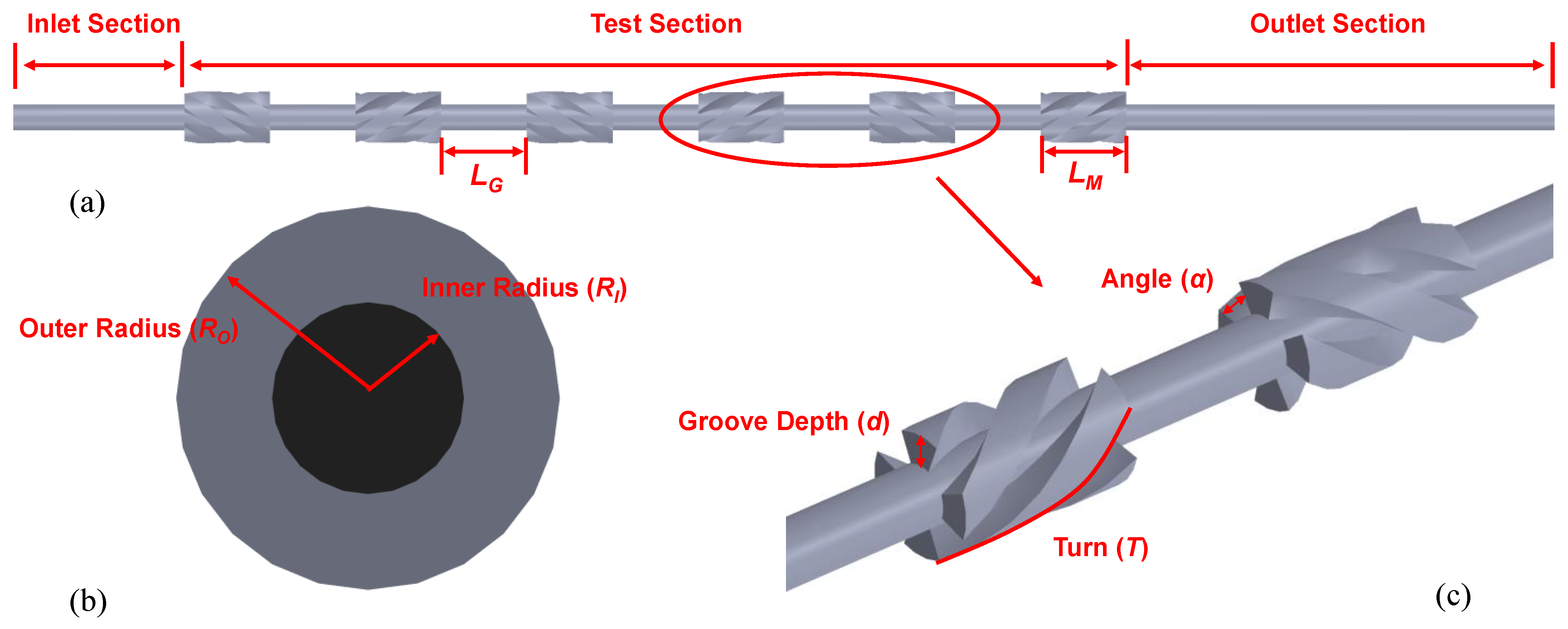
3.1. 3D-Printed Split-and-Recombine Millimeter-Scale Reactor

The equipment for studying the modified model is a tubular split and recombination reactor, whose physical model is illustrated in Figure 2a,b. A central annular tube with an outer diameter of 6 mm ( R O ) and an inner diameter of 3 mm ( R I ) comprises the reactor. It has a series of split and recombination mixing elements with a diameter of 6 mm and a length of 10 mm ( L M ), distributed uniformly at intervals of 10 mm ( L G ) along the circular tube. The structure has four twisted grooves uniformly rotating along the circumference for fluid passage. Two adjacent twisted grooves are separated at 90 degrees on the cross-section of the tube. The physical structure of the reactor can be obtained using 3D printing technology, with a processing accuracy less than 0.05 mm.
The tubular reactor consists of three sections: inlet, test, and outlet. The inlet section, 20 mm long, is designed to ensure the complete development of the fluid. These two mixing streams are introduced at equal velocity there, with one entering the reactor through a 3 mm central tube, and the other entering through the remaining annular tube. Thus, the initial flow ratio of these two streams will be 1:3. The test section is 110 mm long, an adequate length to achieve various mixing patterns. The outlet section is 40 mm long, sufficient to stabilize the outlet flow.
Based on the results obtained from the pre-experiments, the angle ( α ), groove depth ( d ), turn ( T ) , and flow rate ( F ) of the reactor significantly affect the flow field and mixing performance in the reactor. These parameters are shown in Figure 2c. Angle denotes the rotation angle of the groove in the mixing element; groove depth represents the depth of the groove; turn refers to the degree of one groove twist. If T = 1 , the groove rotates 360° in a single mixing element. We selected these parameters for numerical simulation and experimental study and set several discrete points for each parameter, which are listed in Table 1.

3.2. Numerical Simulation

To investigate the influence of different structural parameters and inlet flow rates on pressure drop and the energy dissipation rate in the reactor, we conducted 3D steady-state numerical simulations. Water was chosen as the working medium and modeled as a Newtonian, incompressible fluid. The simulations were performed at 20 °C and it is assumed that physical properties, such as viscosity, remain constant. Since the mixing element is placed horizontally in a tube with an inner diameter of 6 mm, we assume that the effect of gravity is negligible. With these assumptions, the momentum governing equations of the fluid are as follows.
u i x i = 0
ρ u i x i + ρ u i u j x j = p x i + x j ( μ u i x i + p τ j i ) ( i = 1 ~ 3 )
where ρ is the density of mixture fluid; u is the internal velocity field; p is the local pressure field; μ is the viscosity of the mixture fluid; and τ j i is the Reynold stress tensor. Here, the SST k-ω model was applied. The range of the Reynold number in this study was from 658 to 5821. The SST k-ω model can be applied to the cases with relatively lower Reynold numbers, which can reproduce the transition from laminar to turbulent flow regimes. Furthermore, for the flow ejected from the curved grooves of the mixing elements, where the fluid has a high-velocity gradient within the boundary layer, the SST k-ω model will be more applicable.
In this study, ANSYS fluent 2020R1, a commercial software based on the finite volume method, was used for the numerical simulations and CFD-Post for post-processing. The SIMPLE algorithm was applied for pressure–velocity coupled solution calculations while the PRESTO! method was used to perform gradient and pressure discretization. The second-order upwind algorithm spatially discretized the momentum, turbulent kinetic energy, and turbulent dissipation rate. The convergence criteria are less than 10−6 for the continuity and momentum equations.
In the simulations, there is difficulty calculating the turbulent kinetic energy, energy dissipation rate, etc., accurately, so, obtaining these results requires higher quality discrete meshes. Therefore, the grid independence test and algorithm reliable verification are necessary to be carried out, which are shown in the Supplementary Materials.

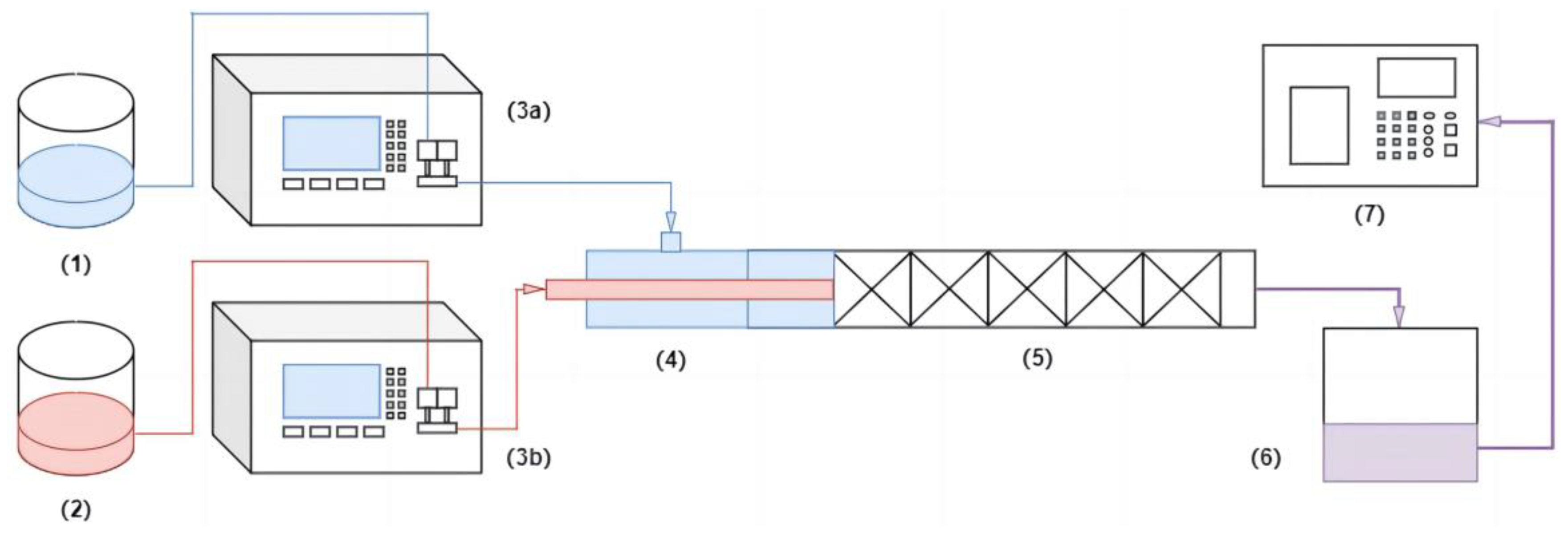
3.3. Mixing Performance Experiments

To quantitatively evaluate mixing performance, classical Villermaux–Dushman experiments [26,27,28] were conducted. We considered the approximate micromixing time range in this case and used the concentration groups of substances provided by J.M. Commenge’s study [29,30,31]. The concentrations of each reagent are presented in Table 2.
The experimental setup diagram is depicted in Figure 3. Iodide-iodate-borate buffer solution and sulfuric acid solution were supplied to the reactor through two HPLC pumps from the outer and central tubes, respectively. The outer and central tubes were connected by commercial T-connectors. To minimize error, three independent samples were taken in each experiment and analyzed by UV-VIS. Finally, the concentration of each species was obtained by subsequent data processing, then XS (segregation index) was calculated. For further details on the Villermaux–Dushman method [32,33,34], please refer to the Supplementary Materials.

3.4. Data Reduction

Based on the set of ordinary differential equations given in Section 2, the independent variables that need to be imported to the reaction model include the inlet flow rate, reaction kinetics, flow time, micromixing characteristic time and mesomixing characteristic time. Apart from the inlet flow rate and reaction kinetics, the calculation of the remaining three variables is given below.
The flow time can be calculated by dividing the reactor length by the average flow velocity in the reactor as follows:
t = L u m
In such SAR reactors, additional attention needs to be taken with respect to D , because the shape of the flow channels in the circular cross section is not regular and the reactor characteristic sizes cannot be determined by conventional methods. Therefore, the hydrodynamic diameter calculation method was used [35]:
D = 4 V S
where V   is the fluid domain volume in the reactor and S is the area which contacts with the fluid in the reactor.
The Reynolds number represents the relative relationship between the inertial and viscous forces in the fluid and is expressed as follows:
R e = ρ u m D μ
where u m is the average velocity along the flow direction.
Baldyga and Bourne [36,37,38,39] proposed an engulfment model to describe micromixing behavior, which is based on the premise that the engulfment of small-scale eddies generates interlaced laminar structures between the micromixing fluid and the environment. These structures promote the deformation of fluid layers that accelerates the aggregate size reduction up to the diffusion scale then intensifies the molecular diffusion between the fluid layers. Based on this theory, the micromixing characteristic time can be determined from numerical simulation using the following equation [40]:
t m = E 1 = 17.3 ( v / ε ) 0.5
Here, the engulfment rate, E , is the inverse of t m , which is related to the energy dissipation rate ε and the dynamic viscosity ν . It is important to note that this empirical formula (Equation (11)) for calculating the micromixing characteristic time requires more validation through comparison with experimental results, which are detailed in the Supplementary Materials.
Additionally, the energy dissipation rate is directly related to the evaluation index of mesomixing [11,41]. According to the theory of inertial-convective disintegration of large-scale eddies, the fluid element’s intermediate scale shrinks from the initial Λ c to the Kolmogorov scale through turbulence dispersion. The whole process constitutes mesomixing [38,41,42,43]. Based on this theory, the mesomixing characteristic time can be estimated using statistical method [12]:
t d = 2 ( Λ C 2 ε ) 1 3
The initial scale of mesoscopic mixing, Λ c , for two streams with the same inlet flow velocity can be calculated by the following equation [11]:
Λ c = ( V B π u ) 0.5
where V B is the volume flow rate of the stream that has a relatively lower flow rate.
The energy dissipation rate refers to energy loss in the fluid due to its essential viscosity and the turbulence induced. The turbulent energy dissipation rate can be related to the velocity strain rate tensor by:
ε = 1 2 v ( u i x j + u j x i ) 2
This tensor can be obtained directly from CFD simulations.

3.5. Optimization Procedure

The optimization method for reactors using GPR, BO, and the modified model is presented in the flowchart shown in Figure 4. In this study, 100 initial design points about the reactor were obtained using the Latin hypercube sampling method. CFD simulations were carried out to determine parameters such as the energy dissipation rate. The reaction kinetics and modified models were then incorporated into a self-programmed 4th-order Runge–Kutta MATLAB program for calculations, acquiring 100 sets of yield and pressure drop data for fitting. These yield and pressure drop data, as performance functions, were mapped to performance metrics by a specific design. This design was defined by a set of structural and operating parameters and subjected to regression validation and optimization in the next step.
In each iteration, a surrogate model was calculated using the known correspondence between the four reactor parameters and the three dependent variables (two product yields plus pressure drop). The next set of parameters, whose mapping value will get closer to the maximum yield and the lowest pressure drop, was chosen by the acquisition function. This parameter set was further used for numerical simulation to obtain the new pressure drop and yields. The cycle of updating the model was repeated. An evaluation index K was defined to determine the final multi-objective optimization results.
K = Y B Y A Y A Δ P B Δ P A Δ P A
Specifically, K is calculated as the ratio of the percentage yield improvement to the percentage pressure drop improvement between two adjacent iteration points, A and B. This metric indicates the amount by which the yield improves when the unit pressure drop increases. If K is less than 5%, we select the current design point as the final multi-objective optimization result based on the optimization principle of GPR-BO.

4. Results and Discussion

4.1. Validation of Modified Model Accuracy

The present study acquired experimental and simulated yields using parallel competing reactions in the classical Villermaux–Dushman method. The yields obtained from both the modified meso-micromixing interaction reaction model and the reaction model containing only the micromixing time term were compared with the experimental results. The results are presented in Figure 5.
The figure shows that the yields obtained from the modified meso-micromixing interaction reaction model are in good agreement with the experimental results, with a maximum relative error of only 3% (Figure 5b). This indicates the accuracy of this modified model for yield prediction. However, the reaction model with the micromixing time term only has a much larger error in the experimental results, particularly at high flow rates, where the relative error can reach up to 14.7% (Figure 5c). This can be attributed to mesomixing becoming the rate-limited step gradually, which is evident from Figure 5, showing that the ratio of micromixing time to mesomixing time, Q , decreases with increasing flow rates. Growing flow rates increase the overall energy dissipation. However, the rate of mesomixing triggered by turbulent dispersion cannot catch up with that of micromixing, and, thus, becomes the rate-limited step [44]. In conclusion, this modified meso-micromixing interaction reaction model is an accurate approach for obtaining yields and can subsequently be used for the optimization in Section 4.3.

4.2. Effect of Parameters on Mixing

4.2.1. Effect of Turn

In Figure 6, the reactor’s full domain energy dissipation rate and segregation index were evaluated at various turns for a fixed groove depth of 1.5 mm and angle of 45°, while the inlet flow rates were also varied. The results indicated a decreasing trend in energy dissipation rate and segregation index with an increase in T , which was found to be more pronounced at lower flow rates. At a flow rate of 150 mL/min, XS for a T of 0.4 was 0.03911, which was 40.4% lower than that for a T of 0.4 with an XS value of 0.06564. However, XS variation at higher T did not become that significant, especially when T = 0.4 and 0.6, as there was almost no difference, with a maximum difference of less than 5%.
The helical motion of the fluid caused by the increased radial velocity component and extended flow path, both in the empty annular space between the two mixing elements and the twisted grooves in the mixing elements, was responsible for this trend (Figure 6b2). At the same time, the strong rotational effect increased the contact area between relatively high and low flow velocity zones in the twisted grooves (Figure 6c2). However, although further increase in T indeed lengthened the flow path, excellent mixing could be achieved right in the middle of the path due to more frequent contact with the fluid. Therefore, extending the flow path or increasing the radial velocity more significantly had a limited effect on improving mixing performance [45]. Overall, these findings highlight the importance of selecting the appropriate turn for optimal reactor performance.

4.2.2. Effect of Inlet Flow Rates

Figure 5 illustrates the decreasing trend of XS with increasing inlet flow rates, from a maximum of 0.05331 to 0.01911. For T > 0.4 and at lower flow rates ( F < 200   mL / min ), XS decreased significantly with increasing flow rate, from 0.06464 to 0.02352, representing a change of 63.6%. However, at higher flow rates, the change in XS leveled off until it concentrated around 0.0123 at a flow rate equal to 400 mL/min.
This trend was mainly attributed to the increasing energy dissipation rate in the annular space between the two mixing elements as the flow rates increased. As shown in Figure 7a1,a2, the flow pattern remained largely unchanged with increasing flow rates, but the overall velocity was significantly affected. This increased velocity leads to a higher degree of turbulence and contact frequency with the fluid, thereby substantially increasing the energy dissipation rate in the annular space (Figure 7b1,b2). However, the effect of higher flow rates on the energy dissipation rate in the annular space is minimal, resulting in a slow improvement in mixing performance. Overall, high flow rates are beneficial for enhancing mixing performance in the reactor.

4.2.3. Effect of Cross-Sectional Area of the Grooves

Angle and groove depth are important factors that determine both the width and depth of grooves in the mixing element, respectively. These two factors together determine the cross-sectional area of grooves, which affects the flow pattern and mixing performance in the annular space and twisted grooves.
Given T = 0.4 , F = 300   mL / min , the reactor’s energy dissipation rate and segregation index varied with groove depth and angle, as presented in Figure 8. Decreasing the cross-sectional area of the groove led to a significant reduction in XS. The maximum XS of 0.0258 was obtained at α = 75 ° and D = 2.5   mm , while a minimum XS of 0.00426 was observed at α = 30 ° and   D = 1   mm , overall resulting in an 83.5% decrease in XS.
Reducing the cross-sectional area of the groove leads to a jet with higher velocity, which spreads out into the annular space to form a rotating plume flow. As this plume moves away from its source, its edges entrain the surrounding fluid, causing the plume to expand further then promoting mixing (Figure 8b2). The energy dissipation rate increased significantly when the cross-section area of the groove became small, from 1.46 m2/s3 at α = 45 ° and D = 1.5   mm to 8.39 m2/s3 at α = 30 ° and D = 1   mm . This can be explained by the fact that the flow area is reduced by a factor of 2.25 and the velocity of the ejected plume increases exponentially, leading to an accelerated improvement in mixing performance. In conclusion, reducing the cross-sectional area of the groove improves the mixing performance of the reactor.

4.3. Optimization Calculations

4.3.1. Optimization Objectives

The objective of this work is to maximize the target product yield and minimize pressure drop by optimizing the reactor parameters. The information about the relevant consecutive reaction is presented in Table 3. The reactor is fed with two streams, A and B, which enter from a 3 mm diameter center tube and annular space with a 6 mm outer diameter and 3 mm inner diameter, respectively. To satisfy the demand for different products in the consecutive reaction, the yields Y 1 and Y 2 of product C and product E, as well as the pressure drop, were chosen as the optimization objectives, while the angle, groove depth, turn and flow rate were selected as the corresponding optimization parameters.
BO is applied to obtain the local minimum value [46]. Therefore, the yields of both products in the consecutive reaction were multiplied by (−1) to transform the optimization problem into a maximization problem, as shown in the following expression:
Objectives :   f 1 ( α ,   d ,   T ,   F ) = { Δ P S A R , Y 1 }   and   f 2 ( α ,   d ,   T ,   F ) = { Δ P S A R , Y 2 }
Subjected   to :   α     [ 15 , 75 ] ;   d     [ 0.5 , 2 ] ;   S     [ 0 , 1 ] ;   F     [ 100 , 400 ]

4.3.2. Results of Gaussian Process Regression

Two commonly used metrics to evaluate a data regression are the mean square error ( M S E for short) and the coefficient of determination ( R 2 for short), which are defined as:
M S E = 1 N i = 1 N ( Y i ,   G P R Y i ) 2
R 2 = 1 i = 1 N ( Y i ,   G P R Y i ) 2 i = 1 N ( Y i ¯ Y i ) 2
A GPR that has a smaller M S E and a larger R 2 is considered more reliable and accurate. Three separate GPRs were utilized to fit the data of Δ P S A R , Y 1 , and Y 2 . To assess the effectiveness of GPR for the regression, an additional analysis was conducted using an artificial neural network (ANN) with multilayer perception (MLP). The tanh function was employed as the activation function in the ANN, which has been widely used in this context [19,47,48,49]. The final trained ANN had a configuration of 5:14:12:2 after double hidden layers were used. Both the regression results of ANN and GPR were compared with results obtained by the reaction model (short for RM), whose normalized values are presented in Figure 9 and Table 4.
In Figure 9, the deviations of three dependent variables for RM, ANN, and GPR are presented. The maximum relative errors for Y 1 and Y 2 were 3.52% and 5.75%, respectively, when using GPR. On the other hand, while ANNs generally meet accuracy requirements, there were several outliers that deviated significantly from the CFD calculations, resulting in maximum errors of 29.62% and 36.86% for Y 1 and Y 2 , respectively.
Table 4 shows that both the M S E and R 2 values in GPRs were significantly better than those in ANNs, indicating that GPR can provide more accurate data and is, therefore, more suitable for fitting in this case. This is because GPR can quantitatively predict uncertainty in a more principled way than ANN, which is particularly relevant for conditions with excessive degrees of freedom. Moreover, by selecting a specific kernel function, GPR can be considered equivalent to an ANN with an infinite number of hidden nodes [50]. However, high accuracy requires more computational resources, although, for just 100 design points, the computational time remains relatively short.

4.3.3. Results of Bayesian Optimization

After obtaining regression results for GPRs, Bayesian optimization was subsequently performed to optimize the reactor parameters.
The optimization process is determined as a multi-objective optimization when the target product is the intermediate product C. To improve the yield of C, the mixing performance needs to be enhanced to disperse the reagent B in the reactor quickly, which reduces its local concentration and slows down the second and third reactions, thereby accumulating product C and reducing the formation of subsequent products, D and E. However, improving the mixing performance requires a higher energy dissipation rate of the fluid, resulting in a higher pressure drop in the reactor. Therefore, a compromise solution between higher intermediate product yields and a relatively lower reactor pressure drop needs to be achieved.
Using Bayesian optimization, a series of Pareto front points were obtained, as shown in Figure 10. These optimization points were evaluated using the metric K   presented in Section 3.5. The desired points with K = 2.92 % were identified with a red circle in Figure 10. Therefore, for the intermediate product C, the maximum yield was 92.5% with a pressure drop in the reactor of 510.50 Pa, where α = 32.8 ° , d = 2.36   mm , T = 0.215 , and F = 145.7   mL / min .
When the target product is the product in the last reaction, E, the process becomes a single-objective optimization. To increase the yield of E, the mixing performance needs to be worsened, resulting in the intermediate product C being diffused to the enriched B region, further reacting with it. This is particularly significant when the residence time of the species becomes longer, as it leads to a higher selectivity of E. A lower energy dissipation rate results in poorer mixing, but also keeps the pressure drop low. Therefore, there is no trade-off or coordination required between the product yield in the last reaction and the pressure drop in the reactor. Optimization is straightforward in that the solution containing both the lowest pressure drop and the highest yield is desired.
A series of optimal points were obtained by Bayesian optimization, as shown in Figure 11. The three leftmost points in the figure are indeed close in value, with a relative difference of less than 0.2%, indicating that the single-objective optimization has reached the limit of iterations. The point identified with the red circle is the desired point, where we acquired the lowest pressure drop and the highest yield. Thus, for the product in the last reaction, the highest yield was 94.3%, with a pressure drop in the reactor of 253.81 Pa, where α = 48.3 ° , d = 2.04   mm , T = 0.344 , and F = 120.37   mL / min .
We have developed an active reactor design method based on CFD-GPR-BO that is applicable to the analysis of different types of reactions, accounting for a meso-micromixing interaction reaction model. In practice, it may be acceptable for a reactor to have a higher pressure drop to achieve the most desired yields as long as the pressure drop is within a reasonable and allowable range. Nevertheless, this method still provides valuable guidance for practical applications, including reactor development for different types of reactions, significantly reducing the reactor design time.

5. Conclusions

In summary, the present study has led to the following conclusions:
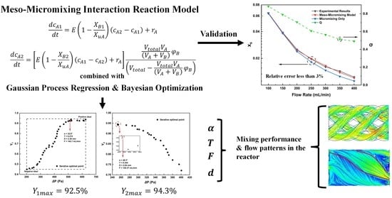
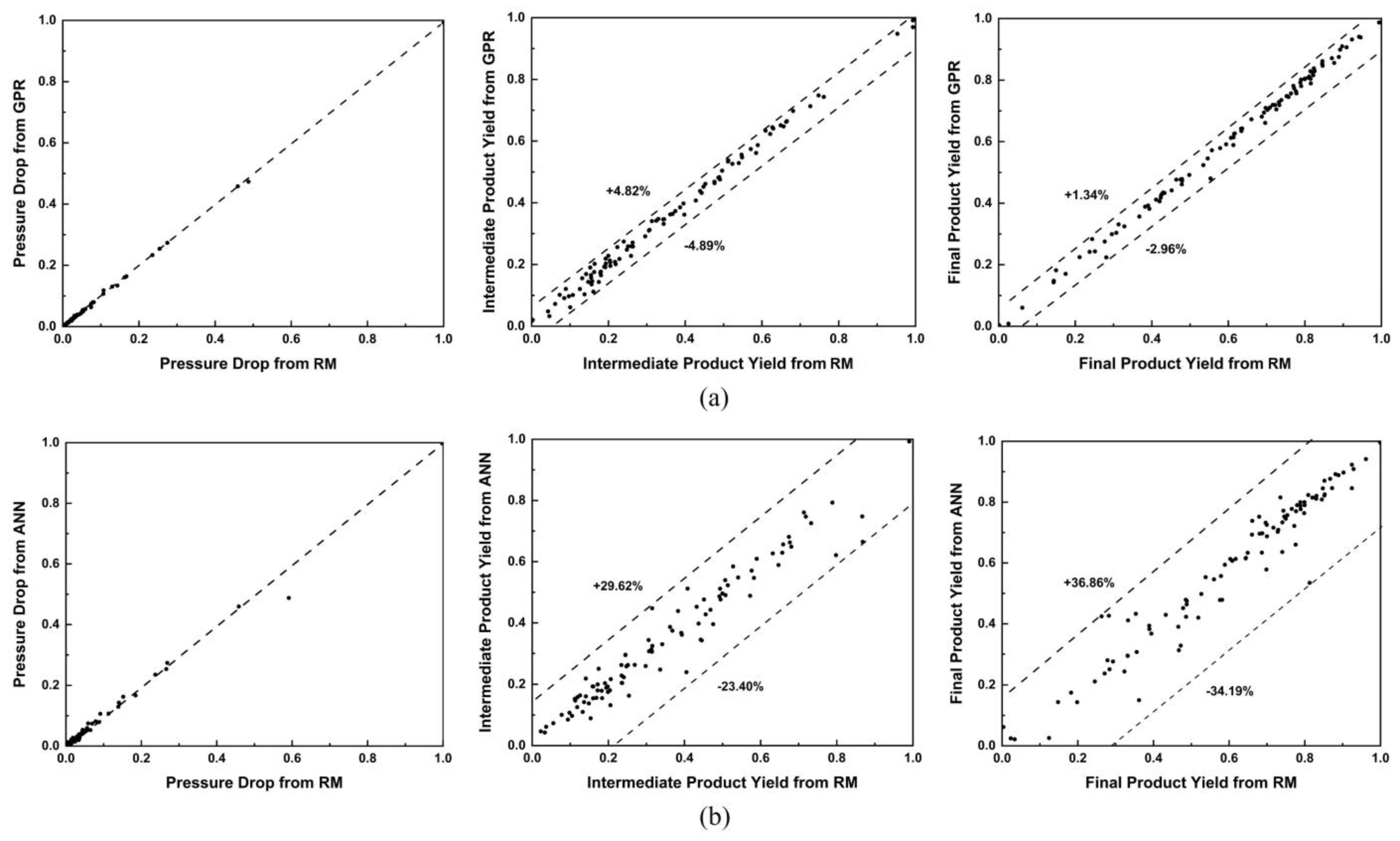
  • A modified meso-micromixing interaction reaction model was developed based on the flow characteristics in continuous reactors. The model was validated by comparing experimentally obtained yields with those predicted by this model. The modified model significantly reduced error in predicted product yields from approximately 15% to within 3%, compared to the model containing the micromixing term only.
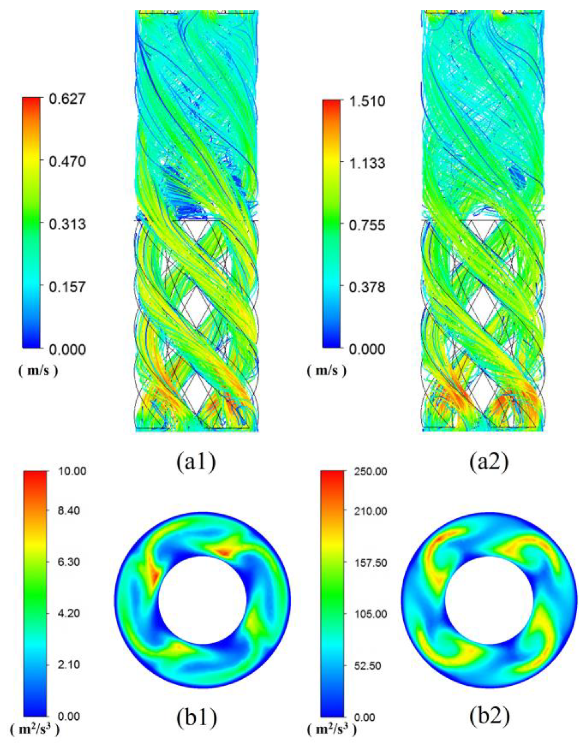
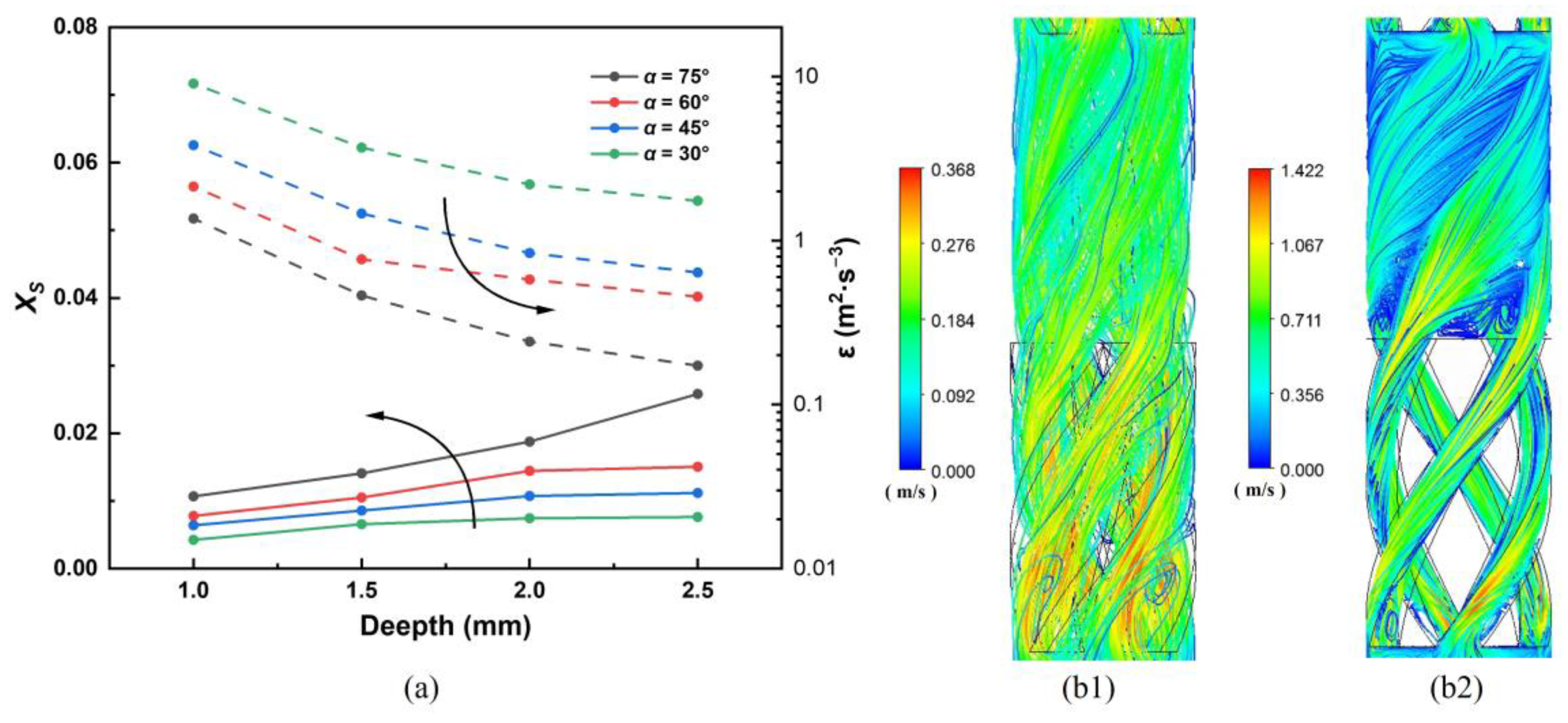
  • Mixing performance in the reactor was improved by characterizing the decreasing XS with increasing flow rate, the degree of twist in the mixing element’s grooves, and the decreasing cross-sectional area of grooves. A high flow rate intensifies the energy dissipation of the fluid in the annular space between two mixing elements; high turn extends the flow path and increases the contact area between the areas with high and low flow velocities in the twisted grooves. When the cross-sectional area in the grooves becomes small, a significant plume flow can be formed in the annular space, improving mixing performance.
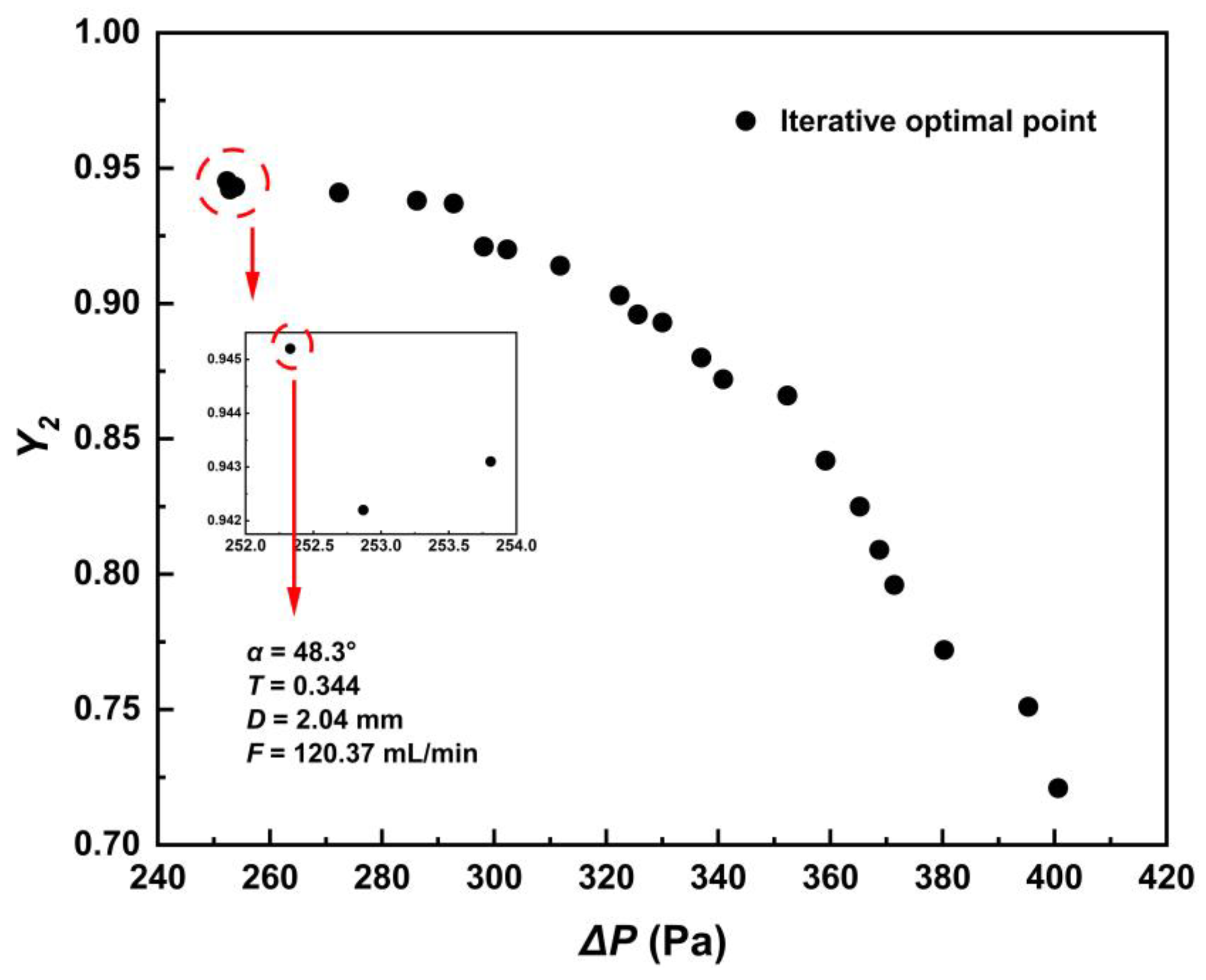
  • The optimization, in which the yields of target products and pressured drop in the reactors were chosen as the optimization objectives, was based on the modified model and performed by BO along with GPR. We obtained the highest product yield while keeping the pressure drop low. For the intermediate product, the yield was 92.5%, while the pressure drop in the reactor was 510.50 Pa. For the product in the last reaction, the yield was 94.3%, while the pressure drop in the reactor was 253.81 Pa. The corresponding combinations of reactor parameters were obtained. This kind of optimization method can be applied to the design of various reactors, providing a reference for structural selection and operational parameter determination.

Supplementary Materials

The following supporting information can be downloaded at: https://www.mdpi.com/article/10.3390/pr11051576/s1. Supporting information is available on model accuracy verification, mesh independence test, and the principles of the Villermaux−Dushman method, Gaussian process regression and Bayesian optimization.

Author Contributions

Conceptualization, methodology, CFD simulation, validation, formal analysis, writing—original draft preparation, writing—review and editing, J.J.; CFD simulation, formal analysis, supervision, N.Y.; Conceptualization, methodology, H.L. and J.T.; validation, C.W.; supervision, R.W. and X.Y. All authors have read and agreed to the published version of the manuscript.

Funding

This research is funded by the Jiangsu Seven Continents Green Chemical Co., Ltd.

Institutional Review Board Statement

Not applicable.

Informed Consent Statement

Not applicable.

Data Availability Statement

The data can be found in the supporting information.

Conflicts of Interest

The authors declare no conflict of interest.

Nomenclature

A N N Artificial neural network, for short
B O Bayesian optimization, for short
c i The mole concentration of component i, mol/m3
d Groove depth, mm
D The hydrodynamic diameter of the reactor cross-section, m
E The engulfment rate in terms of micromixing, s−1
E D R Energy dissipation rate, for short
F Flow rate, mL/min
G P R Gaussian process regression, for short
K Criteria for multi-objective optimization
L G Distance between two mixing elements, mm
L M Length of a mixing element, mm
M S E Mean square error, for short
P Local pressure field, Pa
Δ P S A R Pressure drop in the full domain of reactors
r i Intrinsic reaction rate of component i, mol/(m3·s)
R I Outer radius of tube-in-tube reactors, mm
R O Inner radius of tube-in-tube reactors, mm
R 2 Coefficient of determination
R e Reynold number
S Skewness of curved grooves
S A R Split-and-recombine reactor, for short
t d Mesomixing characteristic time, s
t m Micromixing characteristic time, s
u Local velocity field, m/s
u m Average velocity along the flow direction, m/s
V Volume of the reactor fluid domain
X 0 Ratio of initial flow rates in a tubular reactor
X B Volume of micromixed fluid relative to the whole fluid
X u Volume fraction which contains the partially segregated fluid as islands, embedded in a sea
Y 1 Intermediate product yield
Y 2 Final product yield
z Axial position of the reactors, m
Greek symbols
α Circulation angle, °
ε Energy dissipation rate, m2/s3
Λ c Average from the integral scale of concentration fluctuations to Kolmogorov scale
μ Dynamic viscosity of the fluid, Pa·s
ν Kinematic viscosity of the fluid, Pa·s
ρ Density of the fluid, kg/m3
φ B Ratio of fluid volume change after micromixing

References

  1. Berton, M.; de Souza, J.M.; Abdiaj, I.; McQuade, D.T.; Snead, D.R. Scaling continuous API synthesis from milligram to kilogram: Extending the enabling benefits of micro to the plant. J. Flow Chem. 2020, 10, 73–92. [Google Scholar] [CrossRef]
  2. Hughes, D.L. Applications of Flow Chemistry in the Pharmaceutical Industry—Highlights of the Recent Patent Literature. Org. Process. Res. Dev. 2020, 24, 1850–1860. [Google Scholar] [CrossRef]
  3. Nagaki, A.; Yoshida, J.-I. Controlled Polymerization in Flow Microreactor Systems. In Controlled Polymerization and Polymeric Structures: Flow Microreactor Polymerization, Micelles Kinetics, Polypeptide Ordering, Light Emitting Nanostructures; Abe, A., Lee, K.-S., Leiber, L., Kobayashi, S., Eds.; Springer: Berlin/Heidelberg, Germany, 2013; pp. 1–50. [Google Scholar]
  4. Parua, S.; Sikari, R.; Sinha, S.; Chakraborty, G.; Mondal, R.; Paul, N.D. Accessing Polysubstituted Quinazolines via Nickel Catalyzed Acceptorless Dehydrogenative Coupling. J. Org. Chem. 2018, 83, 11154–11166. [Google Scholar] [CrossRef] [PubMed]
  5. Paul, E.L.; Treybal, R.E. Mixing and product distribution for a liquid-phase, second-order, competitive-consecutive reaction. AIChE J. 1971, 17, 718–724. [Google Scholar] [CrossRef]
  6. Bourne, J.R.; Ravindranath, K.; Thoma, S. Control of product distribution in mixing-controlled reactions. J. Org. Chem. 1988, 53, 5166–5168. [Google Scholar] [CrossRef]
  7. Rys, P. The Mixing-Sensitive Product Distribution of Chemical Reactions. Chimia 1992, 46, 469. [Google Scholar] [CrossRef]
  8. Christy, P.F.; Ridd, J.H.; Stears, N.D. Nitration of bibenzyl by nitronium tetrafluoroborate. Comments on the mechanism of nitration by nitronium salts. J. Chem. Soc. B Phys. Org. 1970, 797–801. [Google Scholar] [CrossRef]
  9. Cox, S.M. Chaotic mixing of a competitive–consecutive reaction. Phys. D Nonlinear Phenom. 2004, 199, 369–386. [Google Scholar] [CrossRef]
  10. Baldyga, J.; Bourne, J.R.; Dubuis, B.; Etchells, A.W.; Gholap, R.V.; Zimmermann, B. Jet Reactor Scale-Up for Mixing-Controlled Reactions. Chem. Eng. Res. Des. 1995, 73, 497–502. [Google Scholar]
  11. Bourne, J.R. Mixing and the Selectivity of Chemical Reactions. Org. Process. Res. Dev. 2003, 7, 471–508. [Google Scholar] [CrossRef]
  12. Bałdyga, J.; Bourne, J.; Hearn, S. Interaction between chemical reactions and mixing on various scales. Chem. Eng. Sci. 1997, 52, 457–466. [Google Scholar] [CrossRef]
  13. Samant, K.D.; Ng, K.M. Development of liquid-phase agitated reactors: Synthesis, simulation, and scaleup. AIChE J. 1999, 45, 2371–2391. [Google Scholar] [CrossRef]
  14. Chin, P.; Barney, W.S.; A Pindzola, B. Microstructured reactors as tools for the intensification of pharmaceutical reactions and processes. Curr. Opin. Drug Discov. Dev. 2009, 12, 848–861. [Google Scholar]
  15. Hessel, V.V.; Gursel, I.V.; Wang, Q.Q.; Noel, T.; Lang, J. Potential Analysis of Smart Flow Processing and Micro Process Technology for Fastening Process Development: Use of Chemistry and Process Design as Intensification Fields. Chem. Eng. Technol. 2012, 35, 1184–1204. [Google Scholar] [CrossRef]
  16. Movsisyan, M.; Delbeke, E.I.P.; Berton, J.K.E.T.; Battilocchio, C.; Ley, S.V.; Stevens, C.V. Taming hazardous chemistry by continuous flow technology. Chem. Soc. Rev. 2016, 45, 4892–4928. [Google Scholar] [CrossRef] [PubMed]
  17. Morse, P.D.; Beingessner, R.L.; Jamison, T.F. Enhanced Reaction Efficiency in Continuous Flow. Isr. J. Chem. 2017, 57, 218–227. [Google Scholar] [CrossRef]
  18. Schlüter, M.; Herres-Pawlis, S.; Nieken, U.; Tuttlies, U.; Bothe, D. Small-Scale Phenomena in Reactive Bubbly Flows: Experiments, Numerical Modeling, and Applications. Annu. Rev. Chem. Biomol. Eng. 2021, 12, 625–643. [Google Scholar] [CrossRef]
  19. Lira, J.O.; Riella, H.G.; Padoin, N.; Soares, C. Computational fluid dynamics (CFD), artificial neural network (ANN) and genetic algorithm (GA) as a hybrid method for the analysis and optimization of micro-photocatalytic reactors: NOx abatement as a case study. Chem. Eng. J. 2022, 431, 133771. [Google Scholar] [CrossRef]
  20. Gambella, C.; Ghaddar, B.; Naoum-Sawaya, J. Optimization problems for machine learning: A survey. Eur. J. Oper. Res. 2021, 290, 807–828. [Google Scholar] [CrossRef]
  21. Stulp, F.; Sigaud, O. Many regression algorithms, one unified model: A review. Neural Netw. 2015, 69, 60–79. [Google Scholar] [CrossRef]
  22. Ryan, E.G.; Drovandi, C.C.; McGree, J.M.; Pettitt, A.N. A Review of Modern Computational Algorithms for Bayesian Optimal Design. Int. Stat. Rev. 2015, 84, 128–154. [Google Scholar] [CrossRef]
  23. Greenhill, S.; Rana, S.; Gupta, S.; Vellanki, P.; Venkatesh, S. Bayesian Optimization for Adaptive Experimental Design: A Review. IEEE Access 2020, 8, 13937–13948. [Google Scholar] [CrossRef]
  24. Zuhal, L.R.; Amalinadhi, C.; Dwianto, Y.B.; Palar, P.S.; Shimoyama, K. Benchmarking multi-objective Bayesian global optimization strategies for aerodynamic design. In Proceedings of the 2018 AIAA/ASCE/AHS/ASC Structures, Structural Dynamics, and Materials Conference, Kissimmee, FL, USA, 8–12 January 2018. [Google Scholar]
  25. Park, S.; Na, J.; Kim, M.; Lee, J.M. Multi-objective Bayesian optimization of chemical reactor design using computational fluid dynamics. Comput. Chem. Eng. 2018, 119, 25–37. [Google Scholar] [CrossRef]
  26. Guichardon, P.; Falk, L. Characterisation of micromixing efficiency by the iodide–iodate reaction system. Part I: Experimental procedure. Chem. Eng. Sci. 2000, 55, 4233–4243. [Google Scholar] [CrossRef]
  27. Guichardon, P.; Falk, L.; Villermaux, J. Characterisation of micromixing efficiency by the iodide–iodate reaction system. Part II: Kinetic study. Chem. Eng. Sci. 2000, 55, 4245–4253. [Google Scholar] [CrossRef]
  28. Gobert, S.R.L.; Kuhn, S.; Braeken, L.; Thomassen, L.C.J. Characterization of Milli- and Microflow Reactors: Mixing Efficiency and Residence Time Distribution. Org. Process. Res. Dev. 2017, 21, 531–542. [Google Scholar] [CrossRef]
  29. Feng, Y.; Zhang, H.; Wang, J.; Yang, Y. Performance Evaluation and Scale-Up Behavior of an Engineered In-Line Mixer for 3D Printing. Ind. Eng. Chem. Res. 2021, 60, 11568–11578. [Google Scholar] [CrossRef]
  30. Martínez, A.N.M.; Chaudhuri, A.; Assirelli, M.; van der Schaaf, J. Effects of increased viscosity on micromixing in rotor–stator spinning disk reactors. Chem. Eng. J. 2022, 434, 134292. [Google Scholar] [CrossRef]
  31. Commenge, J.-M.; Falk, L. Villermaux–Dushman protocol for experimental characterization of micromixers. Chem. Eng. Process. Process. Intensif. 2011, 50, 979–990. [Google Scholar] [CrossRef]
  32. Arian, E.; Pauer, W. A comprehensive investigation of the incorporation model for micromixing time calculation. Chem. Eng. Res. Des. 2021, 175, 296–308. [Google Scholar] [CrossRef]
  33. Wenzel, D.; Assireli, M.; Rossen, H. On the reactant concentration and the reaction kinetics in the Villermaux-Dushman protocol. Chem. Eng. Process.-Process Intensif. 2018, 130, 332–341. [Google Scholar] [CrossRef]
  34. Fournier, M.C.; Falk, L.; Villermaux, J. A new parallel competing reaction system for assessing micromixing efficiency—Experimental approach. Chem. Eng. Sci. 1996, 51, 5053–5064. [Google Scholar] [CrossRef]
  35. Khalde, C.M.; Ramanan, V.; Sangwai, J.S.; Ranade, V.V. Passive Mixer cum Reactor Using Threaded Inserts: Investigations of Flow, Mixing, and Heat Transfer Characteristics. Ind. Eng. Chem. Res. 2020, 59, 3943–3961. [Google Scholar] [CrossRef]
  36. Baldyga, J.; Bourne, J. A fluid mechanical approach to turbulent mixing and chemical reaction part II micromixing in the light of turbulence theory. Chem. Eng. Commun. 1984, 28, 243–258. [Google Scholar] [CrossRef]
  37. Bałdyga, J.; Bourne, J. Interactions between mixing on various scales in stirred tank reactors. Chem. Eng. Sci. 1992, 47, 1839–1848. [Google Scholar] [CrossRef]
  38. Baldyga, J.; Bourne, J. Simplification of micromixing calculations. I. Derivation and application of new model. Chem. Eng. J. 1989, 42, 83–92. [Google Scholar] [CrossRef]
  39. Bałdyga, J.; Pohorecki, R. Turbulent micromixing in chemical reactors—A review. Chem. Eng. J. Biochem. Eng. J. 1995, 58, 183–195. [Google Scholar] [CrossRef]
  40. Ghanem, A.; Lemenand, T.; Valle, D.D.; Peerhossaini, H. Static mixers: Mechanisms, applications, and characterization methods—A review. Chem. Eng. Res. Des. 2014, 92, 205–228. [Google Scholar] [CrossRef]
  41. Baldyga, J.; Bourne, J.; Yang, Y. Influence of feed pipe diameter on mesomixing in stirred tank reactors. Chem. Eng. Sci. 1993, 48, 3383–3390. [Google Scholar] [CrossRef]
  42. Villermaux, J.; Falk, L. A generalized mixing model for initial contacting of reactive fluids. Chem. Eng. Sci. 1994, 49, 5127–5140. [Google Scholar] [CrossRef]
  43. Ertesvåg, I.S.; Magnussen, B.F. The Eddy Dissipation Turbulence Energy Cascade Model. Combust. Sci. Technol. 2000, 159, 213–235. [Google Scholar] [CrossRef]
  44. Martínez, A.N.M.; Jansen, R.; Walker, K.; Assirelli, M.; van der Schaaf, J. Experimental and modeling study on meso- and micromixing in the rotor–stator spinning disk reactor. Chem. Eng. Res. Des. 2021, 173, 279–288. [Google Scholar] [CrossRef]
  45. Woldemariam, M.; Filimonov, R.; Purtonen, T.; Sorvari, J.; Koiranen, T.; Eskelinen, H. Mixing performance evaluation of additive manufactured milli-scale reactors. Chem. Eng. Sci. 2016, 152, 26–34. [Google Scholar] [CrossRef]
  46. Shields, B.J.; Stevens, J.; Li, J.; Parasram, M.; Damani, F.; Alvarado, J.I.M.; Janey, J.M.; Adams, R.P.; Doyle, A.G. Bayesian reaction optimization as a tool for chemical synthesis. Nature 2021, 590, 89–96. [Google Scholar] [CrossRef] [PubMed]
  47. Lv, J.; Liu, Z.; Liu, W. Active design for the tube insert of center-connected deflectors based on the principle of exergy destruction minimization. Int. J. Heat Mass Transf. 2020, 150, 119260. [Google Scholar] [CrossRef]
  48. Ofman, P.; Struk-Sokołowska, J. Artificial Neural Network (ANN) Approach to Modelling of Selected Nitrogen Forms Removal from Oily Wastewater in Anaerobic and Aerobic GSBR Process Phases. Water 2019, 11, 1594. [Google Scholar] [CrossRef]
  49. Abdollahi, A.; Shams, M. Optimization of shape and angle of attack of winglet vortex generator in a rectangular channel for heat transfer enhancement. Appl. Therm. Eng. 2015, 81, 376–387. [Google Scholar] [CrossRef]
  50. Neal, R.M. Bayesian Learning for Neural Networks; Springer Science & Business Media: Berlin/Heidelberg, Germany, 2012; Volume 118. [Google Scholar]
Figure 1. Diagram of mixing between two streams with comparable flow rates under continuous conditions. Each stream serves as the reciprocal environmental fluid and their volume flow rates change a lot. (The amount of Δ V A and Δ V B cannot be ignored).
Processes 11 01576 g001
Figure 2. Physical model of SAR reactors: (a) Front view of SAR reactor; (b) Schematic diagram of the annular structure; (c) Geometrical parameters of mixing elements.
Processes 11 01576 g002
Figure 3. Schematic overview of the experimental setup: (1) Sulfuric acid solution container; (2) Buffered solution container; (3a) HPLC pump for sulfuric acid solution; (3b) HPLC pump for buffered solution; (4) Commercial T-joint; (5) SAR reactor; (6) Outflow container; (7) UV−VIS spectrometer. The blue solution represents sulfuric acid solution, the red buffered solution, and the purple the solution after the reaction.
Processes 11 01576 g003
Figure 4. Algorithm of CFD-GPR-BO.
Processes 11 01576 g004
Figure 5. (a) Comparison of the yields obtained by the Villermaux–Dushman method with those obtained by the meso-micromixing interaction reaction model and the model which only consists of micromixing time. (The green dashed line represents the ratio of micromixing time to mesomixing time, Q, as a function of the inlet flow rate); (b) Error lines of yields obtained by experiments and meso-micromixing model; (c) Error lines of yields obtained by experiments and the model only with micromixing term.
Processes 11 01576 g005
Figure 6. (a) Variation in segregated index (XS, a series of solid lines) and volume-average energy dissipation rate in the reactor ( ε , a series of dashed lines) under different flow rates and skewness at d = 1.5 mm and α = 45°; (b) Streamline in a mixing unit set; (c) Velocity contours of cross-sections at z = 42 mm in the twisted grooves. Here, (1) represents the cases with S = 0.2, while (2) with S = 0.8.
Processes 11 01576 g006
Figure 7. Flow pattern information with different flow rates: (a1,a2) Streamline in a mixing unit set; (b1,b2) EDR contours of cross-sections at z = 53 mm. Here, (1) represents the cases with F = 150 mL/min, while (2) with F = 350 mL/min.
Processes 11 01576 g007
Figure 8. (a) Variation in segregated index (XS, a series of solid lines) and volume-average energy dissipation rate in the reactor ( ε , a series of dashed lines) under different D and α at F = 300 mL/min and S = 0.4; (b1,b2) Streamline in a mixing unit set; Here, (1) represents the cases with α = 75° and D = 2.0 mm, while (2) with α = 30° and D = 1.0 mm.
Processes 11 01576 g008
Figure 9. Deviations and maximum relative errors between RM and the two regression methods: (a) results between RM and GPR; (b) results between RM and ANN. Each dot in the figures represents the simulated value and the fitted value. Each dashed line represents the maximum positive or negative relative error of the fitted value.
Processes 11 01576 g009
Figure 10. Pareto front for intermediate product yield obtained by BO and a solution that meets the criteria.
Processes 11 01576 g010
Figure 11. Results of single-objective optimization for the yield of product in the last reaction obtained by BO and a solution which meets the error criteria.
Processes 11 01576 g011
Table 1. Geometrical parameters and flow rate of the tube and inserts.
α , ° d ,   m m T F ,   m L / m i n
15, 30, 45, 60, 750.5, 1, 1.5, 2, 2.50.2, 0.4, 0.6, 0.8, 1100, 150, 200, 250, 300, 350, 400
Table 2. Concentration recipe of reagents for Villermaux–Dushman method.
MaterialsConcentration [mol/L]
H2BO30.09
NaOH0.09
KIO30.006
KI0.032
H2SO40.0026
Table 3. Kinetic and operational information about the competitive consecutive reaction.
Information about the Reactions
A + B C         r 1 = k 1 c A c B  
C + B D         r 2 = k 2 c C c B  
D + B E         r 3 = k 3 c D c B  
k 1 = 50   m 3 / ( mol · s )     k 1 = 20   m 3 / ( mol · s )     k 1 = 100   m 3 / ( mol · s )
V A   : V B = 1 : 3     V M A = V M B = 5   mol / m 3
Table 4. MSE and R 2 of three optimization objectives for GPR and ANN.
GPRANN
M S E R 2 M S E R 2
Δ P S A R 1.40880 × 10−40.945938.51216 × 10−50.99670
Y 1 3.38565 × 10−30.789482.87026 × 10−40.97674
Y 2 3.85881 × 10−30.962881.45477 × 10−40.99972
Disclaimer/Publisher’s Note: The statements, opinions and data contained in all publications are solely those of the individual author(s) and contributor(s) and not of MDPI and/or the editor(s). MDPI and/or the editor(s) disclaim responsibility for any injury to people or property resulting from any ideas, methods, instructions or products referred to in the content.

