Review

Topological Isomorphism of Liquid–Vapor, Fusibility, and Solubility Diagrams: Analogues of Gibbs–Konovalov and Gibbs–Roozeboom Laws for Solubility Diagrams

by
Nikolay A. Charykov
1,2,
Alexey V. Rumyantsev
1,*,
Konstantin N. Semenov
3,
Zhasulan Shaymardanov
4,
Botogyz Shaymardanova
4,
Natalia A. Kulenova
4,
Marzhan A. Sadenova
4,
Ludmila V. Shushkevich
4,
Victor A. Keskinov
1 and
Alexander A. Blokhin
1
1
Saint-Petersburg State Institute of Technology, Technical University, Moskovskii Pr., 26, St. Petersburg 190013, Russia
2
Department of Physical Chemistry, Electrotechnical University «LETI», Prof. Popova Str., 5, St. Petersburg 197376, Russia
3
Department of Solid-State Chemistry, Institute of Chemistry, Saint Petersburg State University, Universitetskii Pr., 26, St. Petersburg 198504, Russia
4
Department of Metallurgy, Center “Veritas”, East Kazakhstan State Technical University, A.K. Protozanov Street, 69, Ust-Kamenogorsk 070004, Kazakhstan
*
Author to whom correspondence should be addressed.
Processes 2023, 11(5), 1405; https://doi.org/10.3390/pr11051405
Submission received: 9 March 2023 / Revised: 24 April 2023 / Accepted: 25 April 2023 / Published: 6 May 2023
(This article belongs to the Section Materials Processes)

Abstract

:
The comprehensive topological isomorphism of liquid–vapor, fusibility, and solubility diagrams in the proper sets of variables is proven with the aid of van der Waals equations of the shift in phase equilibrium. Analogues of Gibbs–Konovalov and Gibbs–Roozeboom laws are demonstrated in solubility diagrams of ternary and quaternary systems under crystallization of different types of solid solutions. For the demonstration, the quaternary reciprocal system K + , NH 4 + | | Cl , Br H 2 O and its ternary subsystems with modeling of the liquid phase within the framework of the classical Pitzer formalism are mainly used. An algorithm for calculating solubility equilibria in these systems is given.

1. Thermodynamics Backgrounds

1.1. Van der Waals Equation of the Shift in Phase Equilibrium in the Metric of Gibbs Potential

Let us consider an n-component heterogenium system and introduce the (n–1)-dimensional vectors of compositions X i = ( x 1 i ,   x 2 i x n 1 i ) , where x j i is mole fraction of the j-th component in the i-th phase.
Let us consider a heterogenium equilibrium between two phases, α and β. The following parameters are independent variables of phase states in the metric of Gibbs potential: temperature, T; pressure, P; and mole numbers of components, n i (or mole fractions). The (α–β) equilibrium shift can be described by the following system of differential van der Waals equations in vector–matrix form in the variables of phase α (Equation (1)) and phase β (Equation (2)), plus an additional equation (Equation (3)):
( X α X β ) G ^ α d X α = S α β d T V α β d P
( X β X α ) G ^ β d X β = S β α d T V β α d P
G ^ α d X α + S α d T V α d P = G ^ β d X β + S β d T V β d P
where V τ and S τ are the molar volumes and entropies of the corresponding phase (τ = α or β); V τ and S τ are the gradients of these properties with respect to concentration, V τ / x i τ T , P , x k τ x i , n τ and S τ / x i τ T , P , x k τ x i , n τ ); X τ is a vector that characterizes the state of the figurative point of the phase τ in the concentration space of system; d X τ is a vector characterizing the displacement of X τ according to displacement of the two-phase equilibrium; G ^ τ is an operator corresponding to the matrix of the second derivatives G i j τ :
G i j τ = 2 G τ x i τ x j τ T , P , x k τ x i , n τ
where G τ is the molar Gibbs energy potential of the phase τ. According to the phase stability criterion, the matrices of the G ^ τ operators and corresponding quadratic bilinear forms are nondegenerate. Additionally, according to the phase diffusion stability criterion, the matrices corresponding to the quadratic bilinear form G ^ τ are defined positively:
d 2 G τ T , P = i = 1 n 1 j = 1 n 1 G i j τ d x i τ d x j τ > 0
and according to Sylvester’s criterion, the following system of determinants (minors of main diagonal) should be determined positively:
Δ n 1 τ = G 1 , 1 τ G 1 , n 1 τ G n 1 , 1 τ G n 1 , n 1 τ > 0 Δ n 2 τ = G 21 τ G 2 , n 2 τ G n 1 , 1 τ G n 1 , n 2 τ > 0 Δ 2 τ = G i i τ G i j τ G j i τ G j j τ > 0 Δ 1 τ = G i i τ > 0
The physical senses of parameters
S α β = S β S α + ( X β X α ) S α S β α = S α S β + ( X α X β ) S β V α β = V β V α + ( X β X α ) V α V β α = V α V β + ( X α X β ) V β
are, correspondently, the entropy and volume changes in the process of the isothermal–isobaric formation of one mole of phase β from an infinitely large mass of phase α, and vice versa.

1.2. Incomplete Gibbs Potential(s) and Van der Waals Equation of Phase Equilibrium Shift in Its Metric

Let us introduce the incomplete Gibbs potential (or Korjinskii’s potential [1]) for an n-component system:
G w = G μ 1 n 1 = i = 2 n μ i n i
where μ i and n i are the chemical potential and mole number of the i-th component. Such potentials can be invented in many ways, but here, we will consider only the case when the first component is a solvent—water, for example—that is, n 1 = n w .
Let us again consider an n-component heterogenium system and introduce the (n − 2)-dimensional vectors of compositions Y i = ( y 1 i ,   y 2 i y n 1 i ) , where y j i is the mole fraction of the j-th component (in the i-th phase) in the concentration space reduced with respect to the mole number of the solvent. These are the Janecke indices of solutes:
y i = n i / j = 2 n n j
The following parameters are independent variables of phase states in the metric of incomplete Gibbs potential (8): temperature, T; pressure, P; Janecke indices, y i ; chemical potential of solvent,   μ w . Similar to the previous one, the (α–β) equilibrium shift can be described by the following system of differential van der Waals equations in the vector–matrix form:
Y α Y β G ^ w α d Y α = S w α β d T V w α β d P + n w w α β d μ w
Y β Y α G ^ w β d Y β = S w β α d T V w β α d P + n w w β α d μ w
G ^ w α d Y α + S w α d T V w α d P + n w w α d μ w = G ^ w β d Y β + S w β d T V w β d P + n w w β d μ w
where V w τ ,   S w τ , or n w w τ are the molar volume, entropies, or solvent mole number of phase τ, which are calculated without taking into account the solvent (per mole solutes). Further, V w τ ,   S w τ ,   n w w τ are the gradients of these properties with reduced concentration, V w τ / y i τ T , P , y k τ y i , n 1 τ , μ w τ , S w τ / y i τ T , P , y k τ y i , n 1 τ , μ w τ , n w w τ / y i τ T , P , y k τ y i , n 1 τ , μ w τ , correspondently; Y τ is a vector, characterizing the state of the figurative point of the phase τ in the solvent-reduced concentration space; d Y τ is a vector characterizing the displacement of Y τ according to displacement of the two-phase equilibrium; G ^ w τ is an operator, corresponding to the matrix of the second derivatives G i j w τ :
G i j w τ = 2 G w τ y i τ y j τ T , P , y k τ y i , n 1 τ , μ w τ
According to the phase stability criterion and Sylvester’s criterion, the reduced analogues of expressions (5) and (6) remain valid:
d 2 G w τ T , P , μ W = i = 2 n 1 j = 2 n 1 G i j w τ d y i τ d y j τ > 0
Δ n 2 w τ = G 1 , 1 w τ G 1 , n 2 w τ G n 2 , 1 w τ G n 2 , n 2 w τ > 0 Δ n 3 w τ = G 2 , 1 w τ G 2 , n 2 w τ G n 2 , 1 w τ G n 2 , n 2 w τ > 0 Δ 2 w τ = G i i w τ G i j w τ G j i w τ G j j w τ > 0 Δ 1 w τ = G i i w τ > 0
Parameters
S w α β = S w β S w α + Y β Y α S w α S w β α = S w α S w β + Y α Y β S w β V w α β = V w β V w α + Y β Y α V w α V w β α = V w α V w β + Y α Y β V w β n w w α β = n w w β n w w α + Y β Y α n W W α n w w β α = n w w α n w w β + Y α Y β n W W β
have the physical senses of entropy, volume, and change in solvent mole number in the isotherm–isobaric-solvent–isopotential process of formation of one mole of phase β from an infinitely large mass of phase α and vice versa in the concentration space, reduced with respect to the mole number of the solvent.
For some additional details and references, see [2].

1.3. Isotherm–Isobaric Solubility Diagram of Ternary Systems. Analogues of Three Gibbs–Roozeboom Rules, Three Gibbs–Konovalov Laws

For fusibility diagrams of binary systems at P = const, the van der Waals Equations (1)–(3) have a very simple form, for example:
x 1 s x 1 l G ^ 1 , 1 s d x s = S s l d T
where s and l denote solid and liquid phases, correspondently. Similarly, for liquid–vapor diagrams of binary systems, we have
x 1 l x 1 v G ^ 1 , 1 l d x l = S l v d T   ( at   P = const )
or
x 1 l x 1 v G ^ 1 , 1 l d x l = V l v d P   ( at   T = const )
The van der Waals equation of the shift in solubility equilibrium (10)–(12) in the ternary system at T, P = const is as follows:
y 1 s y 1 l G ^ 1 , 1 w s d y 1 s = n w w s l d μ w
Equations (17)–(20) in the appropriate variables are isostructural, being S s l > 0 , S l v > 0 , V l v > 0 , and n w w s l > 0 , according to physical sense; and G ^ 1 , 1 s > 0, G ^ 11 l > 0 and G ^ 1 , 1 w s > 0 , according to the criterion of the stability. So, we can formulate analogues of three Gibbs–Roozeboom rules and three Gibbs–Konovalov laws.
First Rule (Law). Mathematically:
dT / dx 1 l P > 0   if   x 1 s > x 1 l
d T / d x 1 l P > 0   and   d P / d x 1 l T < 0   if   x 1 l > x 1 v
In other words, (21): the melting temperature of solid solutions in binary systems at constant pressure increases as the content of the component whose content in the solid solution is higher than in the liquid phase increases; (22): in binary systems, the boiling temperature of solutions at constant pressure and constant temperature decreases as the content of the component whose content in the solution is higher than in the vapor increases.
Analogue:
( d μ w / d y 1 s ) T , P > 0   if   y 1 s > y 1 l
The chemical potential of the solvent (or its thermodynamic activity or partial pressure) at constant pressure and temperature in the ternary system increases as the reduced (calculated without taking into account the solvent) content in the solid solution of the component—whose solventless content in the solid solution is higher than in the liquid solution—increases.
These laws are not of a general nature, and are valid for multicomponent systems only in special cases, which we will discuss below.
Second Rule (Law).
d T / d x 1 l P = 0   if   x 1 s = x 1 l
d T / d x 1 l P = 0   and   d P / d x 1 l T = 0   if   x 1 l = x 1 v
The melting temperature (of both solid solutions and constant composition phases) at constant pressure in a binary system passes through the extremum when the compositions of liquid and solid phases coincide.
When the liquid composition is coincident with the vapor composition, both the boiling point of the solution at constant pressure and its vapor pressure at constant temperature pass through an extremum (binary azeotrope).
( d μ w / d y 1 s ) T , P = 0   if   y 1 s = y 1 l
The chemical potential of the solvent (or its thermodynamic activity or partial pressure) at constant pressure and temperature in the ternary system passes through the extremum when the composition of the liquid phase coinsides with the composition of the solid one in a solvent-free concentration space.
This rule (law) is absolutely general in nature, and is valid for systems with arbitrary numbers of components and any type of phases at equilibrium.
Moreover, at the equilibrium solid phase of constant composition (the formation of a congruently soluble compound on the solubility diagram or the formation of a congruently melting compound on the melting diagram), one can determine the type of extremum, μ w T , P or T P , respectively. It is always maximum. Indeed, let us differentiate, for example, Equation (1):
X l X s G ^ l d X l = S l s d T V l s d P
where d P = 0 , and one passes through the point of the congruently melting compound (distectic), i.e., X l = X s and d X s = 0 :
d X l G ^ l d X l + X l X s G ^ l d 2 X l + X l X s D G ^ l d X l = S l s d T + S l s d 2 T
where operator D G ^ l corresponds to the matrix of the second derivatives D G i j l = G i j l   i 2 in all lines except the first one, where we must set the following members: D G 1 , j l = Δ n 1 l / X j l T , P , x k j , n . Finally, we obtain:
d X l G ^ l d X l = S l s d 2 T
The term d X l G ^ l d X l is positively determined according to the criterion of the binodal stability quadratic form, whereas S l s < 0 . So, ( d 2 T ) P < 0 and T P should pass through the maximum.
It can be proven quite similarly for solubility diagrams that
d Y l G ^ w l d Y l = n w w l s d 2 μ w
and so d 2 μ w T , P < 0 and μ w should pass through the maximum (distonic point).
The solubility diagram of the NaCl–CdCl2–H2O system [3] in coordinates “partial water pressure, Pw, Janecke index of CdCl2, y CdCl 2 ” can be used as an example (Figure 1). It is clear that all three functions—(1) Pw; (2) water activity: a w = P w / P w 0 (where P w 0 is pressure under pure water); (3) chemical potential of water: μ w = μ w 0 + R T ln a w —change in the same direction, so it does not matter which of them will be used to build the solubility diagram.
Another example is the Na + , Cd 2 + | | Cl , S H 2 O quaternary reciprocal system at 25 °C, where the activity of water passes through the maximum at the point of the ternary compound NaCl∙CdSO4∙5H2O (Figure 2, [3]).
Third rule (law).
Let us rewrite Equation (17) for the liquid phase:
x 1 l x 1 s G ^ 1 , 1 l d x l = S l s d T
and Equations (18) and (19) for the vapor phase:
x 1 v x 1 l G ^ 1 , 1 v d x v = S v l d T
x 1 v x 1 l G ^ 1 , 1 v d x v = V v l d P
Let us do the same with Equation (20):
y 1 l y 1 s G ^ 1 , 1 w l d y 1 l = n w w l s d μ w
Let us now divide Equations (31)–(34) into Equations (17)–(20) in pairs. According to Equation (16), effects ( α β ) and ( β α ) have the opposite sign, whereas the second derivatives G i i τ are always positives. Thus, we obtain and prove the following inequalities:
d x 1 s d x 1 l P = S s l S l s G 1 , 1 s G 1 , 1 l > 0 d x 1 v d x 1 l P = S v l S l v G 1 , 1 v G 1 , 1 l > 0 d x 1 v d x 1 l T = V v l V l v G 1 , 1 v G 1 , 1 l > 0 d y 1 s d x 1 l P = n w w s l n w w l s G 1 , 1 w s G 1 , 1 w l > 0
In other words, in binary systems, the compositions of liquid and vapor (both at T = const and at P = const) when moving along the liquid–vapor curve and the compositions of the melt and solid solution (at P = const) when moving along the melting curve always change in the same direction.
Likewise, the compositions of liquid and solid solutions calculated without taking into account the solvent, when moving along the solubility curve in a ternary system (at T, P = const), always change in the same direction.
These laws are not of a general nature, and are valid for multicomponent systems only in special cases, which we will discuss below.

2. Algorithm of Calculation of Ternary Solubility Diagrams under Solid Solution Formation

The cumbersome wording of the considered laws (which become even more confusing in the case of quaternary systems) requires illustrations. For this purpose, we will use the solubility diagram of the reciprocal quaternary system K + , NH 4 + | | Cl , Br H 2 O (and its subsystems), which was chosen due to the following reasons:
  • A large set of data on the concentration dependences of excess thermodynamic functions for all binary subsystems of the quaternary system is available.
  • A large set of data on solubility for all ternary subsystems of the quaternary system (including the composition of equilibrium solid solutions) is also available. Moreover, there is a set of data concerning mixing the thermodynamic functions of binary solid solutions.
  • In the ternary subsystems are realized different types of solid solutions: continuous series, and solid solutions with miscibility gaps.
  • There are excellent (in our opinion) experimental data of solubility for the quaternary system itself, including the composition of ternary solid solutions.
  • In the quaternary system are realized monovariant curves corresponding to the equilibria of saturated liquid with two different solid solutions.
  • Analogues of Gibbs–Konovalov rules and Gibbs–Roozeboom laws may be installed, and demonstrate almost everything by the examples of ternary subsystems and quaternary reciprocal systems when the composition is moving along curves of open evaporation–crystallization, incomplete extrema, and thermodynamic simplification.
The algorithm of calculation (in particular based on the classic Pitzer equations [4,5,6]) of the solubility diagrams for ternary [7,8,9] (this section provides links to some pioneer publications only; the total number of papers on this topic is vast) and quaternary [7,10] systems, quaternary reciprocal systems [7,11], diagonal cuts of quaternary reciprocal systems [12], and more component systems [7,13] with constant composition solid phases has been widely used for several decades.
Articles devoted to the calculation of solubility diagrams under the formation of solid solutions, both in ternary and quaternary systems, are undoubtedly rarer [14,15,16,17,18,19]. This paper contains some generalizations of the last ones.

2.1. Binary Subsystem Treatment

Parameters for the all binary subsystems are summarized in Table 1. They are suitable for the description of full concentration ranges up to saturation. Note that in this paper, the authors did not seek to describe the excess functions of the solutions as accurately as possible. The aim of the work was to illustrate strict thermodynamic laws. In this case, if the model is thermodynamically consistent (as Pitzer’s model is), the parameter sets are not decisive.
Parameters for the KCl H 2 O system were calculated from a smoothed array [20] of experimental data. For the KBr H 2 O system, we used experimental data [21,22,23]. For the NH 4 Cl H 2 O system, we calculated parameters from isopiestic data [24,25]. For the NH 4 Br H 2 O system, we introduced the additional parameter β 2 with the degree value α 2 = 1. The parameter fitting was based on the original data [23,25,26,27], with the obvious dropping points [23,26] discarded and the overlapping data [19,22] used only once.
For all binary subsystems, the standard deviations of the calculated values of osmotic coefficients from experimental ones, σ φ , did not exceed 0.0014.
The thermodynamic potentials of the binary solid phases, calculated taking into account the activity coefficients of all solution components (or logarithms of solubility products, ln SP), are represented in Table 2.

2.2. Ternary Subsystem Treatment

2.2.1. Parametrization of Ternary Liquid Solutions

For three of the four ternary subsystems, isopiestic data on water activity in the region of homogeneous liquid solutions are available in the literature. In the KCl KBr H 2 O [22,30] and KBr NH 4 Br H 2 O [23] systems, water isoactivity lines are straight, i.e., these systems obey Zdanovskii’s rule. In the NH 4 Cl NH 4 Br H 2 O system [25,31], very weak deviations from the straightness of water isoactivity lines are observed, which are comparable with the accuracy of the measurements. It is reasonable to assume that in the KCl NH 4 Cl H 2 O system, the water isoactivity lines will be also straight (or very close to straightness). Accordingly, calculations of Pitzer’s ternary parameters were performed using “artificial arrays” of water isoactivity lines [32]. In all cases, the obtained values of the ternary parameters were very small, less than 0.0006 by module.
As we are going to describe the quaternary reciprocal system NH 4 + ,   K + | | Cl , H 2 O , we need to unify the parameters θ C l , B r and θ K , N H 4 in conjugated ternary systems. We put them equal to zero. Further calculations showed that all other parameters can also be set equal to zero without losing the accuracy of the description of the water activity data. Accordingly, we accepted θ K , N H 4 = θ C l , B r =   Ψ K , N H 4 , C l = Ψ K , N H 4 , B r =   Ψ K , C l , B r = Ψ N H 4 , C l , B r = 0.0 . It is pertinent to note that in the general case, the straightness of the water isoactivity lines does not mean that the Pitzer ternary parameters are zero and vice versa.

2.2.2. Solubility Equilibrium Data for the KCl KBr H 2 O Subsystem

The KCl KBr H 2 O system ranks among the first in the number of publications devoted to the study of solubility diagrams with solid solutions. At 25 °C alone, at least a dozen papers are devoted to this system [33,34,35,36,37,38,39,40,41,42,43,44,45] (in papers [34,38,39,41,45], the composition of the solid phase was not determined). In general, all of the mentioned experimental data are in good agreement with each other; only data [44] are somewhat different. A continuous series of solid solutions, KCl x Br 1 x , are realized in this system. Approximations of phase equilibrium curves by polynomials were carried out in [46,47]; the calculation of the solubility diagram was performed in [48]. Moreover, densities of saturated solutions [33,42,45], densities and parameters of crystal lattice of solid solutions [49]; and some other solution characteristics, for example, enthalpies of crystallization of solid solutions [50], were investigated at 25 °C.
A number of papers were devoted to the calculation of the Gibbs energy of solid solution formation using different methods [51,52,53,54]; these data are in reasonable agreement with each other.

2.2.3. Solubility Equilibrium Data for the NH 4 Cl NH 4 Br H 2 O Subsystem

The NH 4 Cl NH 4 Br H 2 O system was studied in less detail. The experimental solubility data [40,55] refer only to 25 °C. Evidence of these papers is in almost perfect agreement. Data on water pressure under saturated solutions and solid solution densities are also given in [55], while the dissolution heats of solid solutions are given in [31].
The Gibbs free energy of solid solution formation was calculated in papers [31,52,53,55,56]. Data from earlier work [55] suggest that the NH 4 Cl x Br 1 x solid solutions undergo decomposition due to diffusion instability. However, this conclusion has not been confirmed in later works, including by the authors themselves. So, a continuous series of solid solutions is realized in this system.

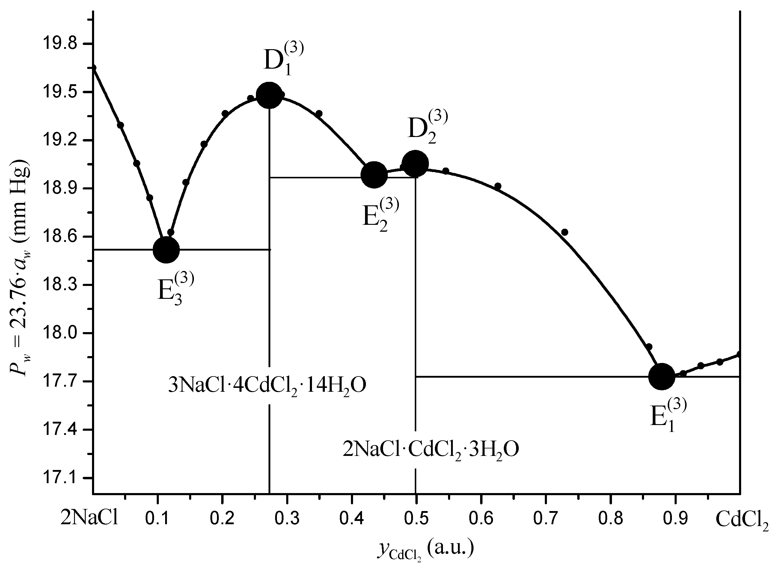
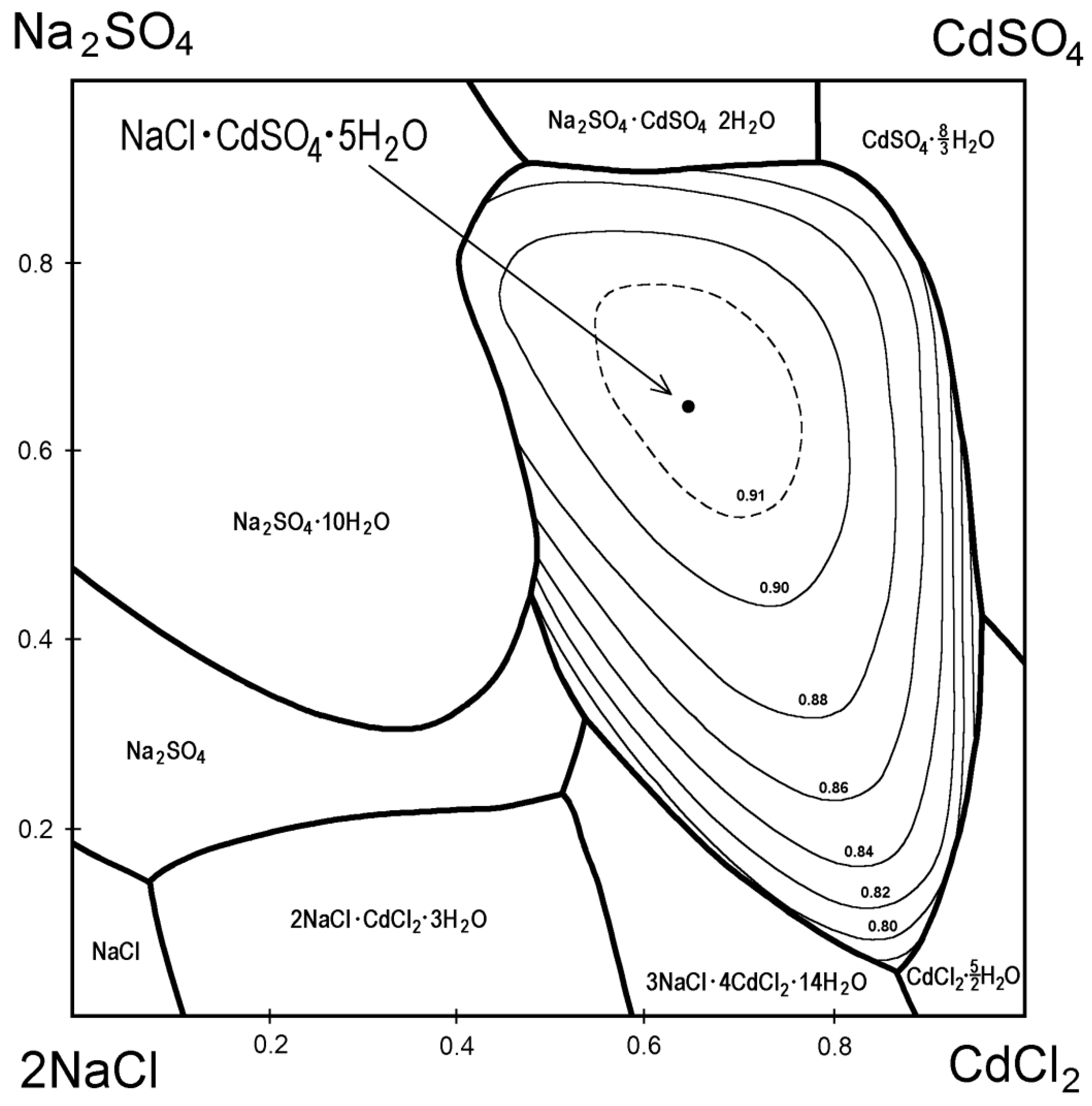
2.2.4. Solubility Equilibrium Data for the KCl NH 4 Cl H 2 O Subsystem

Numerous papers have been devoted to the study of phase equilibria in this system, seven of which contain data at 25 °C [33,40,57,58,59,60,61]. However, in papers [59,61], only the compositions of the liquid phase are presented, while on the contrary, there are no complete data for the liquid phase in paper [61]. In paper [60], the composition of a single point is given, and the data of [33] have a very large scatter and do not agree well with the results of other works. Some data from [59] also fall out of the general set. From the other properties of equilibrium phases in the system, one can note the measurements of the density of saturated solutions in [33,59].
Two series of solid solutions, K x NH 4 1 x Cl and NH 4 x K 1 x Cl , are realized in this system. It is not quite correct to talk about a miscibility gap in a series of solid solutions here, since due to different crystal lattices, these solutions do not have a unified equation of state.

2.2.5. Solubility Equilibrium Data for the KBr NH 4 Br H 2 O Subsystem

Phase equilibria at 25 °C in this system were studied in [33,40,62,63]. A considerable amount of consistent data were obtained, excepting two points from [33]. Note that in paper [62], the recalculation of the composition of “wet residues” into mole fractions of components in the solid phase is performed imprecisely, and in paper [63], it is necessary to combine the data of Table 1 and Table 2 to obtain data on the liquid phase compositions with four significant digits instead of two. Data on the density of saturated solutions are represented in paper [33], and information on water activity in saturated solutions and the calculation of Gibbs energy of solid solution formation is available in paper [63].
Again, two series of solid solutions, K x NH 4   1 x Br and NH 4 x K 1 x Br , are realized in this system.

2.2.6. Algorithm of Ternary Solubility Diagram Calculation

Regardless of the type of crystallizing solid solutions, the first calculation step is to calculate the Gibbs free energy of solid solution formation, ΔG, from the experimental solubility data. In the case of the CA C A H 2 O system, where the ( CA ) X ( C A ) 1 X · ν H 2 O solid solutions are crystallized, we can write:
Δ G R T = x CA · ν H 2 O s ln a CA l ln   S P CA · ν H 2 O s + 1 x CA · ν H 2 O s ln a   C A l ln   S P   C A · ν H 2 O s + ν H 2 O ln   a H 2 O l
where a i l is activity of the i-th salt or water in the liquid phase, x CA · ν H 2 O s is the mole fraction of CA · ν H 2 O in the solid solution. Of course, the same equation is valid, mutatis mutandis, for the CA C A H 2 O system with the ( CA ) X ( C A ) 1 X · ν H 2 O solid solutions, and ν can be equal to zero.
S P Salt · ν H 2 O lattice is the thermodynamic potential of the solid solution component (thermodynamic solubility product), and is defined and is calculated as
ln S P Salt · ν H 2 O lattice = 1 R T μ Salt · ν H 2 O 0 lattice μ Salt · ν H 2 O 0 l = ln a Salt l , sat + ν H 2 O ln a H 2 O l , sat
where the superscript “lattice” emphasizes that the solid solution component possesses the same crystal lattice (syngony) as the solid solution itself (which may correspond to a metastable state); μ Salt · ν H 2 O 0 lattice is its standard chemical potential in a state such as this; μ 0 l is the normalized standard chemical potential of the component in the liquid phase; a i l , sat is the activity of the i-th component in the liquid solution saturated with respect to the solid phase in the aforesaid state. A compound can possess several SPs, but each of them is invariant at fixed T and P. It should be additionally noted that according to the criterion of bimodal and spinodal thermodynamic stability, the solubility of the solid solution components (and the corresponding values of thermodynamic potentials, SP) in the metastable state should always be higher than in the stable state.
At this stage, for systems with a continuous series of solid solutions, the essential point is the need to check the consistency of solubility in binary subsystems and ternary systems and choose consistent values of ln SP; the procedure for such a check is described in [15,64]. It is somewhat more difficult to calculate ΔG in ternary systems under the formation of two series of solid solutions because part of the ln SP values cannot always be directly determined from the binary solubility data. The methods of action in this case are considered in paper [18].
We approximated the determined values of ∆G with a subregular solution model (of course any other model can be used as well):
Δ G e x = Δ G i = KCl , KBr x i s ln x i s = x KCl s x KBr s α 0 + α 1 x KCl s x KBr s
where α 0 and α 1 are adjustable parameters. Strictly speaking, a subregular model was required only for the KCl–KBr solutions; in the other three cases α 1 = 0 , that is, the model of regular solutions, was used—see Table 3. The results of the calculations of ΔG for the systems under consideration are shown in Figure 3a,b.
The subregular model provides us with the activity coefficients of solid solution components, f i s :
R T ln f KCl s = x KBr s 2 α 0 + α 1 3 x KCl s x KBr s R T ln f KBr s = x KCl s 2 α 0 + α 1 x KCl s 3 x KBr s
The final calculations are reduced to solving a system of equations derived from the phase and chemical equilibrium conditions. In the general case, it looks like
ln a CA l + ν H 2 O ln a H 2 O l = ln S P CA · ν H 2 O s + ln a CA · ν H 2 O s ln a   C A l + ν H 2 O ln a H 2 O l = ln S P   C A · ν H 2 O s + ln a   C A · ν H 2 O s
The results of calculations of the liquidus are presented in Figure 4, and the distribution diagrams of the salt components between the equilibrium phases are presented in Figure 5a,b. In the K + | | Cl , Br H 2 O system, both solid phase models reproduce the experimental liquidus well, but the distribution diagram is somewhat better reproduced by the subregular solution model than by the regular solution model.

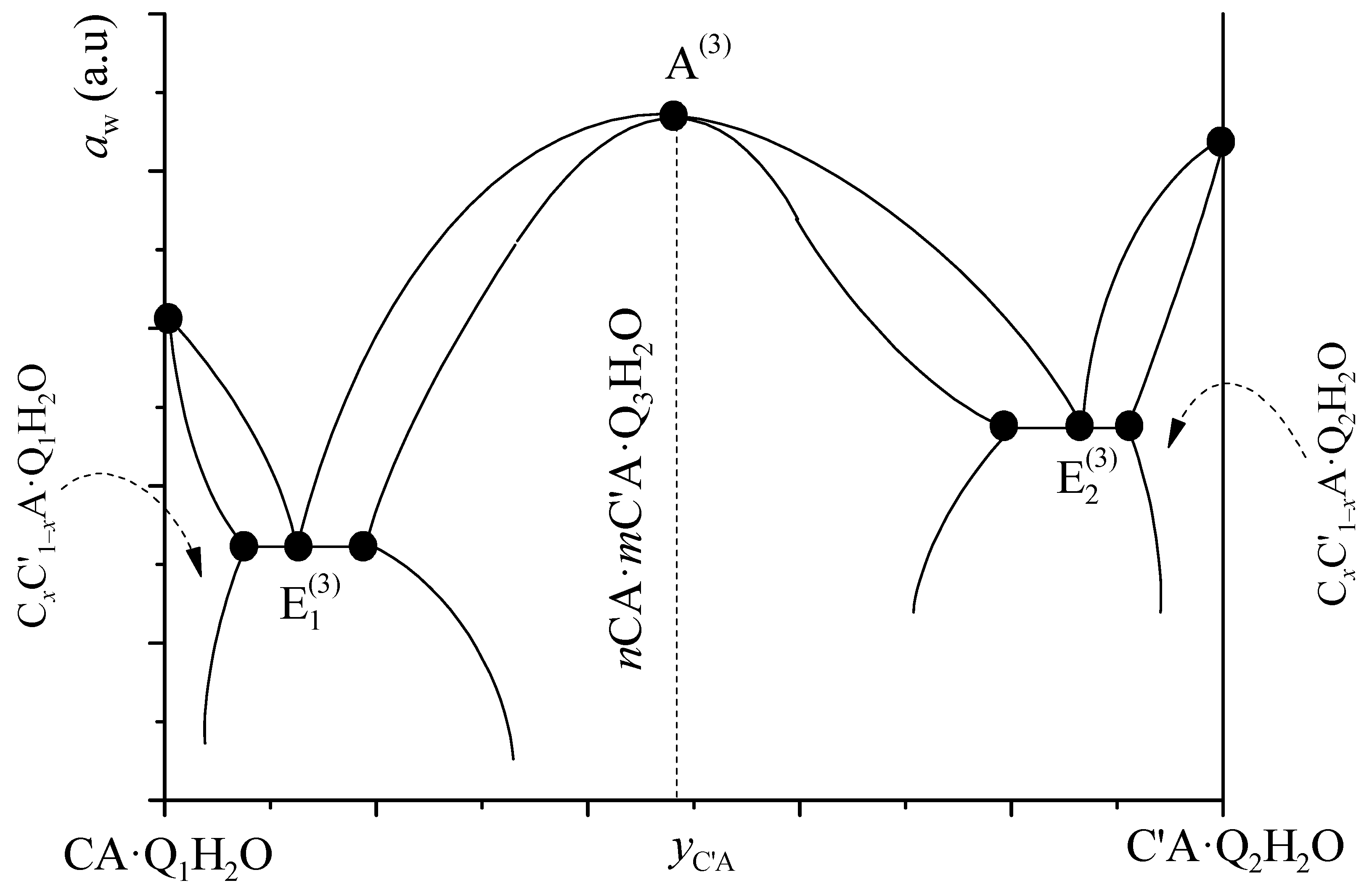
2.2.7. Classification of Solid Solutions on Ternary Solubility Diagrams

Without encroaching on Roozeboom’s classification, in our opinion, it is convenient to distinguish six basic types of solid solutions in the light of the aforesaid work.
  • Types I: Continuous series of solid solutions without miscibility gaps.
This is the most trivial case: the hydrate composition and syngony of both components of solid solutions are the same. SP values can be found from the solubility of components in binary subsystems and ΔG values are calculated in experimental points from Equation (36). The monovariant solubility curve is the geometric place of points that satisfy the system of two nonlinear Equations (40) with respect to three unknown variables, the composition of the saturated ternary liquid solution (for example, CA and C’A molalities), and the mole fraction of one of the solid solution components. Any of these variables can be fixed before solving the system.
According to the derived above analogues of the Gibbs–Roozeboom rules and Gibbs–Konovalov laws, three subtypes are possible.
  • Subtype Ia: Extrema of water activity are absent.
This is a fairly common type, but it is not represented in the ternary systems considered here. Let us consider as an example the diagram of the TbCl3–GdCl3–H2O at 25 °C, Figure 6 [65].
  • Subtype Ib: A minimum of water activity is present.
Two such ternary systems are presented among those considered here, namely KCl KBr H 2 O and NH 4 Cl NH 4 Br H 2 O . For both systems, we calculated stable and metastable variants of the diagram (Figure 7 and Figure 8). In all cases, the minimum water activity in the saturated solutions is realized when the compositions of equilibrium phases in the solvent-reduced concentration space are equal, in full accordance with the analogue of the second Gibbs–Roozeboom rule and Gibbs–Konovalov law. We propose to call such a minimum alyotrope (“α” + “λύω” + “τρόπος”, “no change on dissolving”), by analogy with azeotropes (“α” + “ζέω” + “τρόπος”, “no change on boiling”) in liquid–vapor diagrams.
  • Subtype Ic: A maximum of water activity is present.
There are no such examples in the ternary systems under consideration. Moreover, we looked through the reference data for more than 130 ternary water–salt systems with a continuous series of solid solutions, and could not find a single example where the water activity (or the molar fraction of water, which is almost equivalent) in saturated solutions passes through the maximum.
This is surprising, since for liquid–vapor diagrams and fusibility diagrams of binary systems, which are topologically isomorphic to solubility diagrams of ternary systems [7], diagrams with both minimum and maximum T P x and P T x are well known. This is the only case among all those known to the authors that does not correspond to the postulate of complete topological equivalence of liquid–vapor diagrams, melting diagrams, and solubility diagrams in the corresponding sets of variables.
  • Type II: Discontinuous series of solid solutions with miscibility gaps due to diffusion instability.
In this case, the solubility diagram consists of two curves corresponding to the crystallization of the same solid solution (with the same qualitative (hydrate) composition and uniform syngony) decaying at the nonvariant point due to diffusion instability (this occurs when there are strong positive deviations of the solid solution from ideality). As before, the SP values are available from the binary solubilities of its components, and system (40) describes both curves with 0 x 1 s x 1 lim 1 and x 1 lim 2 x 1 s 1 , where lim1 and lim2 symbolize the broadness of the diffusion instability of the solid solutions and x 1 lim 1 < x 1 s < x 1 lim 2 is the miscibility gap.
As is well known, the equation for the loss of phase diffusion stability (or spinodal curve) for a binary solid solution, s, is as follows:
2 G s x i s 2 T , P = 0   or   μ i s x i s T , P = 0
Within the model of regular (or subregular) solutions, Equation (41) is reduced to an algebraic quadratic (or cubic) equation, which allows one to find both the x 1 lim 1 and x 1 lim 2 roots.
Alternatively, we can calculate the composition of the nonvariant point by solving a system of four equations similar to Equation (40) with respect to two liquid phase composition variables (molalities, for example) and two solid phase composition variables ( x 1 lim 1 and x 1 lim 2 ) .
Moreover, if we have reliable experimental data on the composition of solid solutions at the point of decomposition, we can determine their nonideality parameters directly with Equation (41).
In reality, such a case is rare. However, two (partially metastable) diagrams can be presented for the ternary systems under consideration; see Figure 9 and Figure 10.
  • Type III: Discontinuous (different) series of solid solutions with miscibility gaps due to difference in syngony.
In this case, the solubility diagram also consists of two curves, corresponding to the crystallization of two solid solutions with the same qualitative composition but different syngony. It is more correct to speak not about a miscibility gap, but about two series of different solid solutions, because these solutions do not have a common equation of state in principle.
Here, we have four SP values, two for each of the solid solution components possessing the corresponding crystal lattice. However, only two of them can be determined directly, since in most cases there are no data on the binary solubility of the component in an alien syngony. The missing SP values can be determined simultaneously with fitting the solid phase model parameters from experimental solubility data.
Again, the system of two Equations (40) is suitable for calculating each of the two branches of solubility of solid solutions (each branch has its own system), and the nonvariant point can be calculated by solving the system of four such equations. It is easier, however, to first determine the composition of the solid phases using the following system:
ln S P CA · ν H 2 O s s 1 + ln a CA · ν H 2 O s s 1 = ln S P CA · ν H 2 O s s 2 + ln a CA · ν H 2 O s s 2 ln S P   C A · ν H 2 O s s 1 + ln a   C A · ν H 2 O s s 1 = ln S P   C A · ν H 2 O s s 2 + ln a   C A · ν H 2 O s s 2
where ssi denotes solid solution i. This system reflects the obvious fact that solid solutions are in equilibrium not only with the liquid solution but also with each other. System (42) can also be used to check the experimental data on solubility.
It should be noted that model parameters of the solvent-free solid phase can be determined from indirect data such as solubility in another solvent, fusibility diagrams, or diagrams of the resolution of the solid solution. Sometimes, this requires temperature extrapolation.
Among the ternary systems under consideration, there are two diagrams (stable) of this type; see Figure 11 and Figure 12.
  • Type IV: Discontinuous (different) series of solid solutions with miscibility gaps due to differences in hydrate composition.
In this case, the solubility diagram also consists of two branches corresponding to the crystallization of two solid solutions with different hydrate compositions, whilst their syngony may be the same or may be different. Here, we also should speak of two different solid solutions rather than a miscibility gap, as for type III.
What has been said about the calculation of the solubility diagrams of type III remains valid, except for two peculiarities. First, the missing SP values can often be obtained from the binary solubility diagram of the component with moderate temperature extrapolation. Second, the equations of system (8) turn out not to be decoupled from the liquid phase, since they contain an additional term related to the difference in hydrate composition:
ln S P CA · ν 1 H 2 O s s 1 + ln a CA · ν 1 H 2 O s s 1 = ln S P CA · ν 1 H 2 O s s 2 + ln a CA · ν 1 H 2 O s s 2 ν 2 ν 1 ln a H 2 O l ln S P   C A · ν 2 H 2 O s s 1 + ln a   C A · ν 2 H 2 O s s 1 = ln S P   C A · ν 2 H 2 O s s 2 + ln a   C A · ν 2 H 2 O s s 2 ν 2 ν 1 ln a H 2 O l
As an example, let us present a solubility diagram in the NdCl3–PrCl3–H2O ternary system at 25 °C; see Figure 13 [66].
  • Type V: Internal series of solid solutions.
Two main subtypes can be distinguished here.
  • Subtype Va.
This subtype is caused by the dehydration of solvated solid solutions due to decreasing water activity as the concentration of components in the liquid phase increases. A new solid solution curve with lower water content can “wedge” into the crystallization curve of solid solutions with higher water content. Basic solubility diagrams of this type are shown in Figure 14.
As example of this type of diagram, we can point to the following: the MgSO 4 NiSO 4 H 2 O system at 35 °C, in which a series of Mg x Ni 1 x · 6 H 2 O solid solutions of type Ia appear “inside” a series of the Mg x Ni 1 x · 7 H 2 O solid solutions belonging to type Ia [67,68]; and the CoS O 4 NiSO 4 H 2 O system above 26 °C, in which a series of the Co x Ni 1 x · 6 H 2 O solid solutions of type Ia “lies on” the miscibility gap in a series of the Co x Ni 1 x · 7 H 2 O solid solutions belonging to type III [69,70].
  • Subtype Vb. Solid solutions on the base of a ternary compound (double salt).
As an example, we can consider the solubility diagram of the system MgCl 2 FeCl 2 H 2 O within 40–60 °C, where three series of solid solutions are crystallized: Mg x Fe 1 x Cl 2 · 6 H 2 O based on MgCl 2 · 6 H 2 O , Mg y Fe 1 y Cl 2 · 4 H 2 O based on FeCl 2 · 4 H 2 O , and MgCl 2 z · ( FeCl 2 ) 1 z · 8 H 2 O [71,72,73]. The scheme of the solubility diagram in this case is shown in Figure 15. The calculation algorithm in this case is also preserved, but it should be taken into account that all parameters of the middle solid solution are not available and must be determined by fitting procedure.
  • Type VI: Solid solutions with the variable water content, or so-called “abnormal solid solutions”.
As for solid solutions with variable water content in water–salt systems, there is no consensus in the literature either on the mechanism of their formation or on the components that form them. Some authors even question the very fact of their existence. Accordingly, consideration of such solutions is out of the scope of this paper.

3. Diagrams of Quaternary Reciprocal Systems under Formation of Ternary Reciprocal Solid Solutions

3.1. Backgrounds of Modeling Ternary Reciprocal Solid Solutions

A multicomponent system C ,   C ,   C | | A ,   A , A H 2 O is called reciprocal if at least one reversible chemical reaction can occur:
C A +   C A CA + C A
Here, in general, C ,   C and A ,   A are qualitatively different constituents of substances, such as cations and anions, elements of A3-groups and B5-groups, alcoholic and acidic functional groups, etc.
According to the conditions of chemical equilibrium in a phase of variable composition, the consequence of Equation (44) is the following:
μ CA + μ   C A = μ   C A + μ C A
where μ i is chemical potential of the i-th component in the phase.
In the modeling of the liquid phase on the basis of well-known Friedman axiomatics (most often used in modeling of electrolyte solutions, for example, in the Pitzer model), when the asymmetric normalization of excess thermodynamic functions (in infinitely dilute solution water activity equal to 1 and logarithm of activity coefficient of any salt equal to 0) is used, no additional concordance with Equation (45) is required, since
Δ ln a l = ln a CA l + ln a C A l ln a C A l ln a CA l 0 Δ G 0 l = μ CA 0 l + μ C A 0 l μ C A 0 l μ CA 0 l 0
where a i l and μ i 0 l are the activity and standard chemical potential of the i-th salt in an infinitely dilute solution, and Δ G 0 l is the standard change in the Gibbs energy of reaction (44) in an infinitely diluted solution. Incidentally, to agree with equations such as (46) in calculations in reciprocal systems, we need to unify ternary parameters (such as θ C , C and θ A ,   A in Pitzer equations) in conjugated systems C ,   C | | A H 2 O and C ,   C | | A H 2 O , C | | A , A H 2 O and   C | | A , A H 2 O .
If symmetric normalization (the logarithm of the activity coefficient equals to 0 for any pure component) is used in the modeling in the reciprocal system—as is the case, for example, in the solid solution model—then
Δ ln a s = ln a CA · ν H 2 O s + ln a C A · ν H 2 O s ln a C A · ν H 2 O s ln a CA · ν H 2 O s 0 Δ G 0 s = μ CA · ν H 2 O 0 s + μ C A · ν H 2 O 0 s μ C A · ν H 2 O 0 s μ CA · ν H 2 O 0 s 0
because of the different standard state for pure salts.
The problem of harmonization of the model of reciprocal solid solutions with Equation (45) was solved by one of the authors in papers [74,75] for the case of calculating the fusibility diagrams of reciprocal A3B5 systems. For the ternary reciprocal regular solution of isovalent substitution C x C 1 x | | A y C 1 y · ν H 2 O (ν can be equal to zero as for K x NH 4 1 x Cl y Br 1 y , in our case), we have
μ CA · ν H 2 O s = μ CA · ν H 2 O 0 s + R T ln x y + 1 x 2 y α CA - C A s + 1 y α CA - C A s + 1 y 2 x α CA - CA s + 1 x α C A - C A s + 1 x 1 y Δ G 0 s μ C A · ν H 2 O s = μ C A · ν H 2 O 0 s + R T ln 1 x y + x 2 y α CA - C A s + 1 y α CA - C A s + 1 y 2 x α CA - CA s + 1 x α C A - C A s + x 1 y Δ G 0 s μ CA · ν H 2 O s = μ CA · ν H 2 O 0 s + R T ln x 1 y + 1 x 2 y α CA - C A s + 1 y α CA - C A s + y 2 x α CA - CA s + 1 x α C A - C A s + 1 x y Δ G 0 s μ C A · ν H 2 O s = μ C A · ν H 2 O 0 s + R T ln 1 x 1 y + x 2 y α CA - C A s + 1 y α CA - C A s + y 2 x α CA - CA s + 1 x α C A - C A s + x y Δ G 0 s
where α i j s are the regular model parameters of the binary solid solution of the corresponding syngony (see Table 3). The value of Δ G 0 s arising due to different normalization is easily obtained from the solubility products of the constituents of the solid solution. In fact,
ln S P i = μ i 0 s μ i 0 l R T
and so,
Δ G 0 s Δ ln S P = ln S P CA + ln S P C A ln S P CA ln S P C A

3.2. Calculation Algorithm of Solubility Diagram of Quaternary Reciprocal Systems under Solid Solution Formation

According to the Gibbs phase rule, in a quaternary reciprocal water–salt system at T, P = const, up to three solid solutions can coexist with the liquid phase. Such solid solutions may differ in hydrate composition or in crystalline lattices, or, if the above coincide, have a miscibility gap due to diffusion instability. In general, we can distinguish approximately the same cases as for the ternary systems above.
  • Case I: Continuous series (field) of solid solutions without miscibility gaps.
We were unable to find examples of such diagrams among reciprocal water–salt systems, but they are known for quaternary systems with a common ion ([17], the Mg 2 + , Ni 2 + , Zn 2 + | | SO 4 2 H 2 O system at 25 °C, with the only field of crystallization of the Mg x Ni y Zn 1 x y · 7 H 2 O solid solutions) and for quaternary high-temperature solubility (fusibility) diagrams ([76], the Ga , In , P , As Pb system at 600 °C, where a continuous field of crystallization of the Ga x In 1 x P y As 1 y solid solutions exists). However, any solubility diagram of a reciprocal system always includes exactly such elements, namely the crystallization fields of solid solutions of a certain type.
Let us consider, for example, the two-phase equilibrium in the quaternary reciprocal system K + , NH 4 + | | Cl , Br H 2 O at 25 °C between a liquid phase and the ternary reciprocal solid solutions based on the cubic face-centered lattice, K x + ( NH 4   + ) 1 x Cl y Br 1 y c f c . According to the phase equilibrium conditions, one can write
ln a KBr l = ln S P KBr c f c + ln x y + α K - NH 4 c f c R T 1 x 2 + α Cl - Br c f c R T 1 y 2 + 1 x 1 y   Δ ln S P c f c ln a KCl l = ln S P KCl c f c + ln x 1 y + α K - NH 4 c f c R T 1 x 2 + α Cl - Br c f c R T y 2 1 x y   Δ ln S P c f c ln a NH 4 Cl l = ln S P NH 4 Cl c f c + ln 1 x y + α K - NH 4 c f c R T x 2 + α Cl - Br c f c R T 1 y 2 x 1 y   Δ ln S P c f c
where
α K - NH 4 c f c = y α KCl - NH 4 Cl c f c + 1 y α KBr - NH 4 Br c f c α Cl - Br c f c = x α KCl - KBr c f c + 1 x α NH 4 Cl - NH 4 Br c f c
and
Δ ln S P c f c = ln S P KBr c f c + ln S P NH 4 Cl c f c ln S P NH 4 Br c f c ln S P KCl c f c
The fourth equation ( ln a NH 4 Br l = ) in the system (51) is omitted because it is a linear combination of the first three due to condition (45).
The system of Equation (51) contains five independent variables. Three of them correspond to the composition of the liquid phase (for example, molalities of any three salts, with the fourth molality linked to them by Equation (44) or via the electroneutrality equation), and the other two correspond to solid solution composition. Thus, we describe a bivariate surface of two-phase equilibrium.
We can introduce up to two additional conditions in the numerical solution of the system (51). For example, we can calculate a water isoactivity line in the field of solid solution crystallization by specifying the value a w , or calculate the diagonal cross section of the diagram by setting y K + l = y Cl l , etc.
When using a solid solution model other than the regular one, the problem to be solved is not essentially different.
  • Case II: Series of solid solutions with miscibility gaps due to diffusion instability.
The solubility diagram in this case consists of two fields, corresponding to the crystallization of two solid solutions with the same qualitative composition, and one monovariant curve corresponding to the three-phase equilibrium of the saturated liquid solution with both solid solutions. System (51) is still valid for each of the fields. The monovariant curve can be calculated either by solving the system of six nonlinear equations (three for each solid solution), or as follows.
The loss of diffusion stability in the ternary reciprocal solution corresponds to the condition
2 G s x 1 2 2 G s x 1 x 2 2 G s x 2 x 1 2 G s x 2 2 = 0
where G s is that part of the average molar Gibbs potential of solid solutions whose second derivatives of the composition are nonzero. In our case,
G s R T = x y ln x y + x 1 y ln x 1 y + 1 x y ln 1 x y + 1 x 1 y ln 1 x 1 y + α C - C s R T x 1 x + α A - A s R T y 1 y
This equation yields two monovariant curves corresponding to the marginal compositions of solid solutions.
As an example, we can point to the quaternary high-temperature solubility diagram of the Ga , In , As , Sb Pb system at 500 °C, where the field of crystallization of the Ga x In 1 x As y Sb 1 y solid solutions with the lattice of sphalerite has a miscibility gap.
  • Case III: Two series of solid solutions of the same qualitative composition with different crystal lattice structures.
A perfect example is the solubility diagram of the considered quaternary system K + , NH 4 + | | Cl , Br H 2 O at 25 °C. It consists of two bivariant fields of solid solutions that crystallize in cubic face-centered (cfc) and cubic (cub) lattices, and one monovariant curve corresponding to the crystallization of both solid solutions, K x NH 4 1 x Cl y   Br 1 y c f c and K x NH 4 1 x Cl y   Br 1 y c u b .
Again, system (51) is valid for each of the fields, while the monovariant curve can be obtained by solving the system of six nonlinear equations (three for each solid solution). Alternatively, one can solve a system of three nonlinear equations with respect to the four variables corresponding to the compositions of equilibrium solid solutions, x c f c x 1 ,   y c f c y 1 and x c u b x 2 ,   y c u b y 2 :
ln S P KCl c f c + l n x 1 y 1 + α K - NH 4 c f c R T 1 x 1 2 + α Cl - Br c f c R T 1 y 1 2 + 1 x 1 1 y 1   Δ ln S P c f c = ln S P KCl c u b + l n x 2 y 2 + α K - NH 4 c u b R T 1 x 2 2 + α Cl - Br c u b R T 1 y 2 2 + 1 x 2 1 y 2   Δ ln S P c u b ln S P KBr c f c + ln x 1 1 y 1 + α K - NH 4 c f c R T 1 x 1 2 + α Cl - Br c f c R T y 1 2 1 x 1 y 1   Δ ln S P c f c = ln S P KBr c u b + ln x 2 1 y 2 + α K - NH 4 c u b R T 1 x 2 2 + α Cl - Br c u b R T y 2 2 1 x 2 y 2   Δ ln S P c u b ln S P NH 4 Cl c f c + ln 1 x 1 y 1 + α K - NH 4 c f c R T x 1 2 + α Cl - Br c f c R T 1 y 1 2 + x 1 1 y 1   Δ ln S P c f c = ln S P NH 4 Cl c u b + ln 1 x 2 y 2 + α K - NH 4 c u b R T x 2 2 + α Cl - Br c u b R T 1 y 2 2 + x 2 1 y 2   Δ ln S P c u b
This system reflects the trivial fact that cub and cfc solid solutions are in equilibrium with each other regardless of their equilibrium with the saturated liquid solution.
The results of the calculation of the solubility diagram are presented in the next section.
  • Case IV: Two series of solid solutions of different hydrate compositions.
This case resembles the previous one. Again, system (51) is valid for each of the fields of each solid solution, and the monovariant curve can be obtained by solving the system of six nonlinear equations. However, a system of equations similar to (56) cannot be used due to the appearance of additional terms related to the solvent activity in the liquid phase (compare with Equation (43)).
  • Case V: Series of solid solutions on the base of a ternary compound.
An example of a system with the formation of reciprocal solid solutions based on a compound is the K + , NH 4 + , Mg 2 + | | Cl , Br H 2 O system at 25 °C, where potassium-ammonium-chloride-bromide carnallite ( K x ( NH 4 ) 1 x · MgCl 2 y Br 2 2 y · 6 H 2 O ) crystallizes. The field of its crystallization is also described by a system of equations similar to (51).

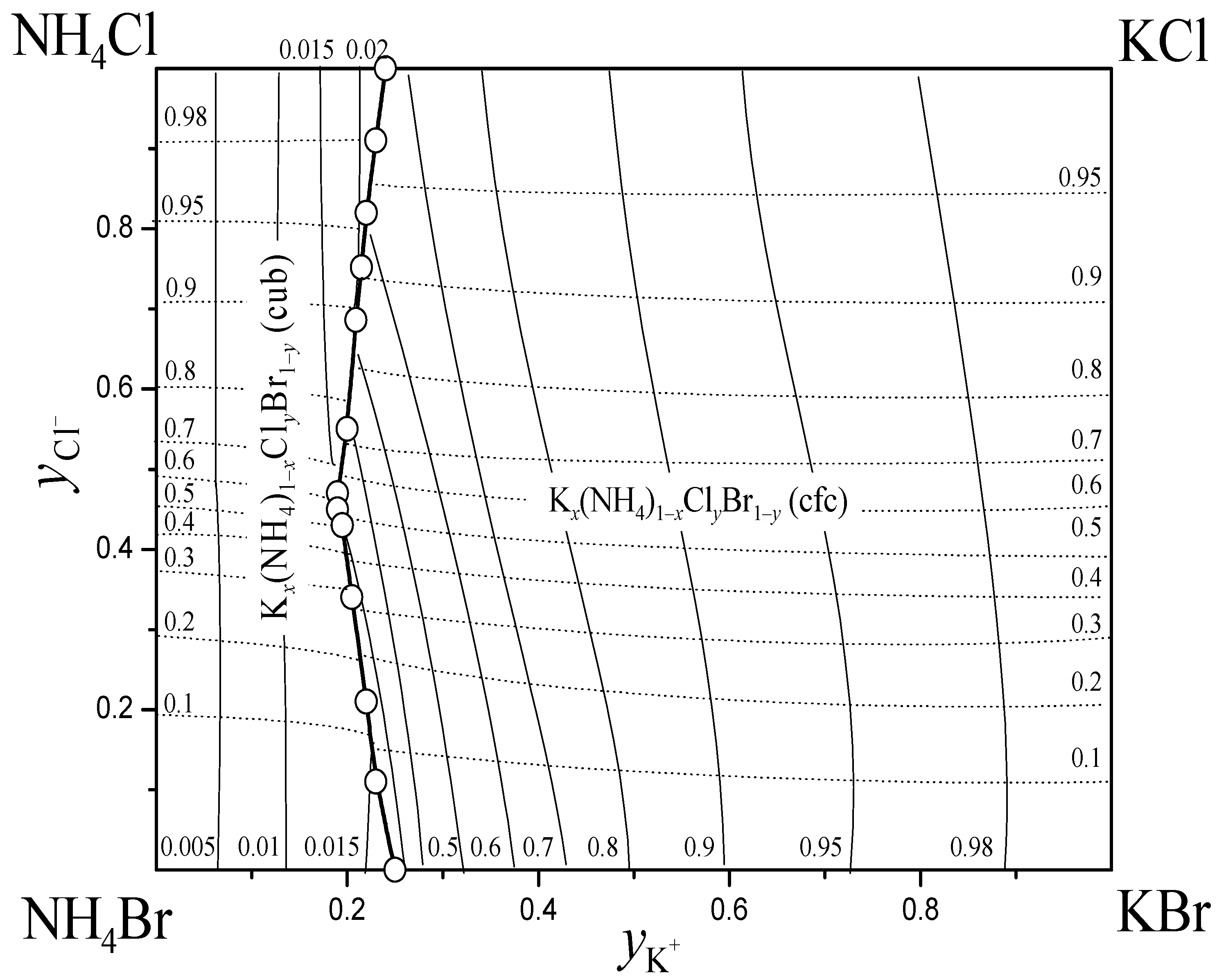
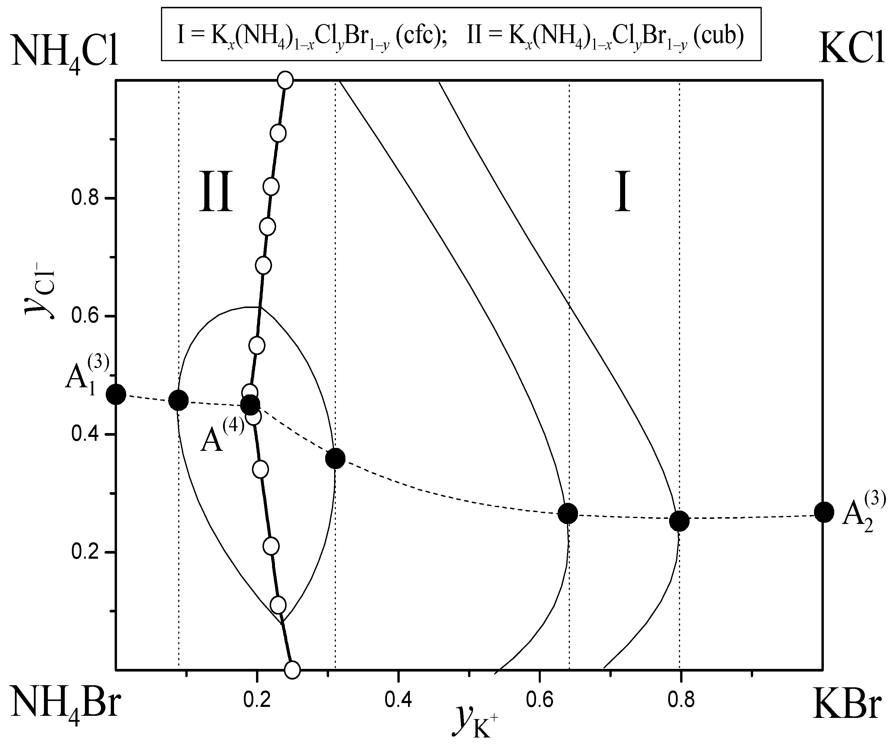
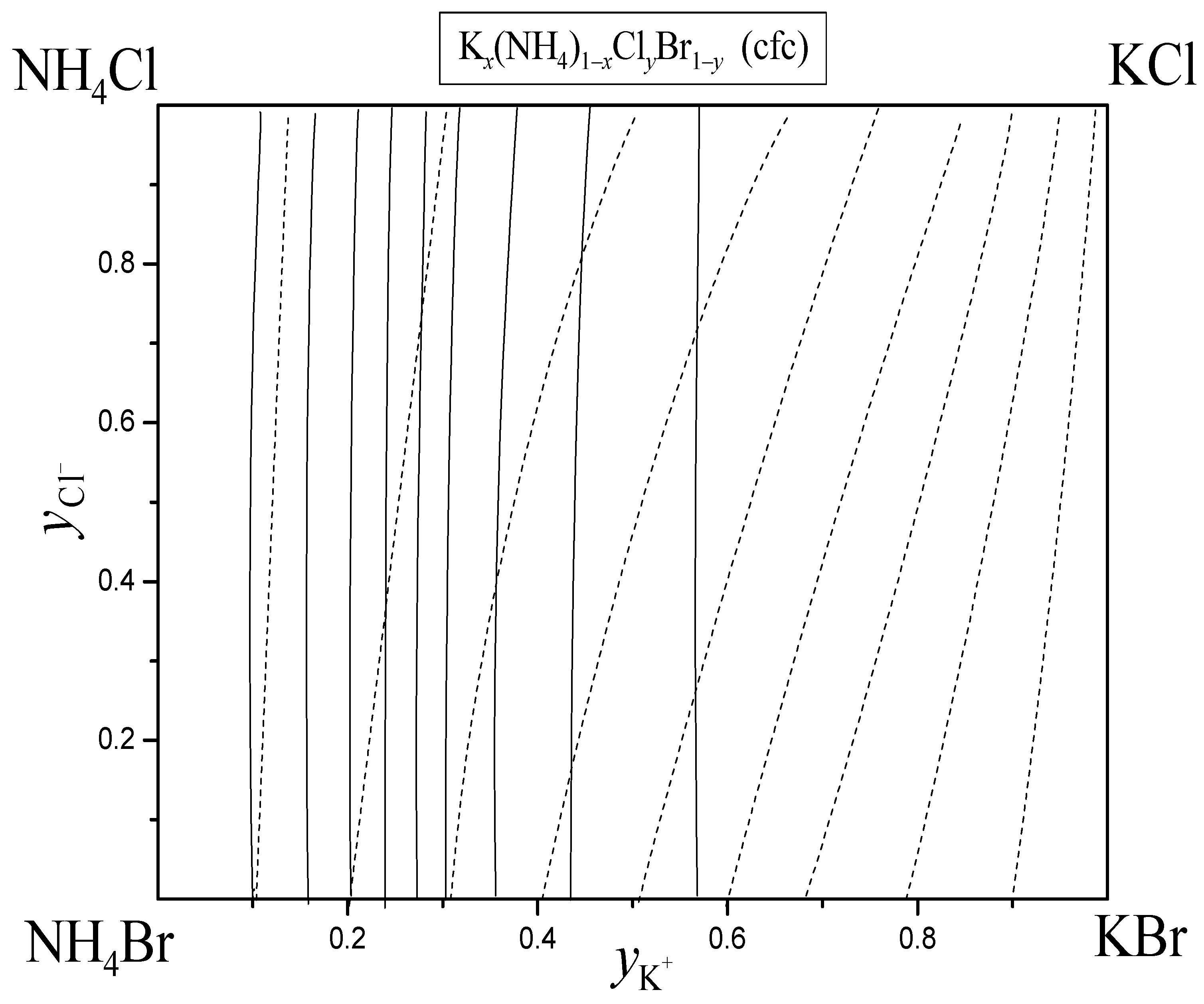
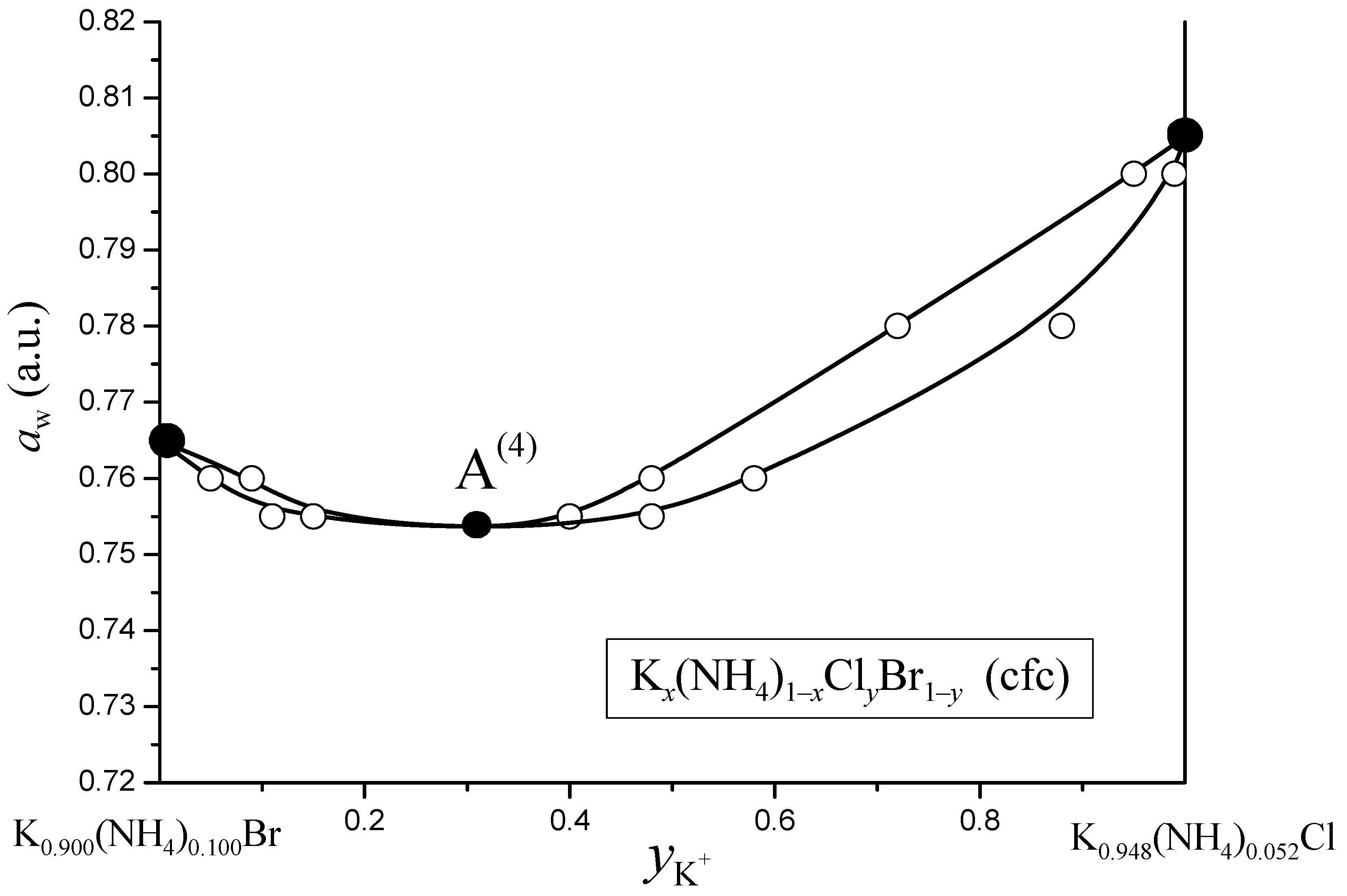
4. Results for the Diagram of Solubility of Quaternary Reciprocal System K + , N H 4 + | | C l , B r H 2 O at 25 °C

The results of the calculation of the solubility diagram of this system in comparison with the available experimental data [77] are shown in Figure 16. There is excellent agreement between the calculation and experiment. Figure 16, Figure 17, Figure 18, Figure 19 and Figure 20 show the results of solving the system of Equation (56) with the imposition of additional conditions: isoconcentrates of cations and anions as well as water isoactivity lines.
All diagrams are shown in the Janecke coordinate system, i.e., as projections of volumetric figures on the plane of the salt components, or in other words, in the solvent-reduced (solvent-free) concentration space:
Y K = m K + m K + + m NH 4 + Y Cl = m Cl m Cl + m Br
where m i denotes molalility of ion i, and m K + + m NH 4 + = m Cl + m Br , according to the electroneutrality equation.
As noted above, the system contains two crystallization fields of ternary reciprocal solid solutions with cubic face-centered and cubic lattices and the monovariant curve of their cocrystallization. The monovariant curves of liquidus and solidus have extremums (minima) of water activity, i.e., there is an incomplete (or conditional) alyotrope. In the solvent-free concentration space, the figurative points of the liquid solution and both solid phases belong to the same straight line at the alyotrope point.

5. Applicability of Analogues of Gibbs–Roozeboom Rules and Gibbs–Konovalov Laws to Multicomponent Systems

Second Rule (Law). As noted already, the analogue of the second law, like its prototype, is universal, and valid for systems with an arbitrary number of components in any way of changing the composition. We will not discuss it further.

5.1. Motion along the Open Evaporation–Crystallization Curves at T = const and P = const

First Rule (Law). The equation of the open evaporation–crystallization process (in other words, the mass balance equation) in the condition of two-phase equilibrium (sl) in the solvent-reduced concentration space has the form:
d Y l = Y s Y l d M s
where d M s is the mass of the solid solution in moles (without taking into account the solvent content), which is formed from 1 mole of liquid phase during evaporation. This means in scalar form:
d y i l d y j l T , P , e v a r c r y s t = y i s y i l y j s y j l
or (numbers k and q are arbitrary)
d y k l = y k s y k l y q s y q l d y q l
As stated earlier, the van der Waals differential equation in the metric of incomplete Gibbs potential (8) and in the liquid phase variables has the form
Y l Y s G ^ w l d Y l = n w w l s d μ w
Let us convert this equation to the scalar form and substitute (60):
i k y i s y i l G ^ w l y k s y k l = n w w l s y q s y q l d μ w d y q l
Since the double sum in the left part is greater than zero according to the stability criteria, and n w w l s is less than zero according to the physical sense,
( d μ w / d y q l ) T , P , e v a r c r y s t > 0   if   y q s > y q l
We proved the analogue of the first rule (law) for diagrams of solubility under the formation of solid solutions in a multicomponent (reciprocal) system:
When moving along a curve of open evaporation–crystallization in a multicomponent (reciprocal) system at constant pressure and temperature, the chemical potential of the solvent increases as the reduced (calculated without taking into account the solvent) content in the solid solution of the component—whose solventless content in the solid solution is higher than in the liquid solution—increases.
In exactly the same way, we can obtain the corresponding rules for motion along a curve of open crystallization on multicomponent (reciprocal) diagrams of fusibility and along curves of open evaporation on multicomponent diagrams of vapor–liquid.
Third Rule (Law). Let us write Equation (62) in the solid phase composition variables
i k y i l y i s G ^ w s y k l y k s = n w w s l y q l y q s d μ w d y q s
and divide one by the other. We immediately obtain
d y q l d y q s T , P , e v a r c r y s t = n w w s l n w w l s
Since n w w l s and n w w s l always have opposite signs according to physical sense,
d y q l / d y q s T , P , e v a r c r y s t > 0
This is an analogue of the third rule (law) for diagrams of solubility under the formation of solid solutions in a multicomponent (reciprocal) system:
Compositions of liquid and solid solutions calculated without taking into account the solvent always change in the same direction when moving along a curve of open evaporation–crystallization in multicomponent (reciprocal) system at constant pressure and temperature.
Of course, corresponding rules for motion along a curve of open crystallization on multicomponent (reciprocal) diagrams of fusibility and along curves of open evaporation on multicomponent diagrams of vapor–liquid are also valid, mutatis mutandis.
Let us illustrate the above with the solubility diagram of the K + , NH 4 + | | Cl , Br H 2 O system at 25 °C. Figure 21 shows the calculation of open evaporation curves, and Figure 22 and Figure 23 present examples of phase diagrams when moving along such curves.

5.2. Motion along the Curves of Incomplete Extrema of Solvent Chemical Potential at T = const and P = const

Let us denote the belonging to the curve of incomplete extrema of the chemical potential of the solvent (or the partial pressure of the solvent) as “inex”. It is known that in the quaternary system, the inex curve is a set of touch points of solvent isotherm–isobar–isopotentials by concentration sections (see Figure 24). Mathematically,
Y l Y s G ^ w l d Y l = 0 d y a l = 0
where a denotes the salt component of the quaternary system (the ion in the reciprocal system), which is absent in the ternary alyotrope and appears only in the incomplete quaternary pseudoalyotropes.
First Rule (Law). For the curve of incomplete extrema, we can easily obtain
Δ 2 w l G 22 w l y a s y a l = n w w s l d μ w y a l T , P , i n e x
Since Δ 2 w l / G 22 w l > 0 , according to the stability criteria, and n w w s l > 0 , according to the physical sense,
( d μ w / d y a l ) T , P , i n e x > 0   if   y a s > y a l
In other words, when moving along the inex curve in a quaternary (reciprocal) system at constant pressure and temperature, the chemical potential of the solvent increases as the reduced (calculated without taking into account the solvent) content in the solid solution of the component—which is absent in the ternary alyotrope, and appears only in the incomplete quaternary pseudoalyotropes whose solventless content in the solid solution is higher than in the liquid solution—increases.
Third Rule (Law). Again, we can rewrite Equation (68) in solid solution variables and divide these two equations by each other:
G 22 w s G 22 w l = n w w s l n w w l s y a l y a s T , P , i n e x
and
y a l y a s T , P , i n e x > 0
In other words, in liquid and solid solutions, the solventless content of the salt (the ion in the reciprocal system) component of the system, which is absent in the ternary alyotrope and appears only in the incomplete quaternary pseudoalyotropes, always changes in the same direction when moving along a incomplete extreme curve in a quaternary (reciprocal) system at constant pressure and temperature.
Illustrations of the rules considered are shown in Figure 25, Figure 26 and Figure 27.
Again, the corresponding rules for motion along a curve of incomplete extrema on ternary (reciprocal) diagrams of fusibility and of vapor–liquid are also valid.
There are two particular points to be made about the analogues of the first and third laws in this case. First, it is impossible to formulate such analogues for those components (ions) of the system that are involved in the ternary alyotrope; Laws I and III are invalid for them. Second, it is impossible to generalize Laws I and III to arbitrary n-component systems (n ≥ 5).

5.3. Motion along the Curves of Thermodynamic Simplification

Thermodynamic simplification curves are lines along which the chemical potentials of two of the three components (in the case of ternary systems) change by equal amounts. Mathematically,
D μ i k = D μ j k
where D μ i k is the differential of the chemical potential of the i-th component of phase k, which takes into account changes in the concentration variables of the phase composition, but not changes of T or P. We will denote such curves as “ t s i j ”.
Let us introduce a thermodynamic simplification curve (e.g., t s 23 ) in a reduced concentration space, and the incomplete Gibbs potential metric
d μ 2 T , P = d μ 3 T , P   or   d μ 2 μ 3 T , P = 0   or   d G w y 2 t s 23 = 0
We have omitted the phase index because this equation can be written in both liquid (l) and solid (s) phase variables according to the phase equilibrium conditions, i.e., t s 23 l t s 23 s . Moreover, the last equality in (73) means that
G 12 w l d y 1 l + G 22 w l d y 2 l = 0
and
G 12 w s d y 1 s + G 22 w s d y 2 s = 0
It is worth noting that thermodynamic simplification curves, unlike, for example, incomplete extrema curves, fill the entire concentration space of the system (see Figure 28 and Figure 29).
First Rule (Law). Substituting (73)–(75) into the van der Waals Equation (61) after simple transformations gives
n w w l s d μ w d y 1 l t s 23 G 22 w l = y 1 s y 1 l Δ 2 w l
where Δ 2 w l = G 11 w l G 12 w l G 21 w l G 22 w l > 0 , according to the stability criteria of the liquid phase, and G 22 w l > 0 and n W w l s < 0 , according to the physical sense. So,
d μ w / d y 1 l t s 23 > 0   if   y 1 s > y 1 l
In other words, when moving along a curve of thermodynamic simplification in a quaternary (reciprocal) system, the chemical potential of the solvent increases as the reduced (calculated without taking into account the solvent) content in the solid solution of the component—whose solventless content in the solid solution is higher than in the liquid solution if such a component does not participate in the condition of thermodynamic simplification—increases.
Third Rule (Law). In exactly the same way as above, we obtain
d y 1 s d y 1 l t s 23 = G 22 w s G 22 w l Δ 2 w l Δ 2 w s n w w s l n w w l s > 0
In other words, when moving along a curve of thermodynamic simplification in a quaternary (reciprocal) system, the content of component—which does not participate in the condition of thermodynamic simplification—changes in liquid and solid solutions in the same direction.
Illustrations of these rules are shown in Figure 30 and Figure 31.
The following is important:
One cannot formulate analogues of Laws I and III for those components that are involved in the thermodynamic simplification condition;
One cannot extend these laws to more component solubility diagrams.

6. Conclusions

Isobaric fusibility diagrams of binary systems with solid solutions in variables “temperature–composition”, liquid–vapor diagrams of binary systems (in variables “temperature–composition” at constant pressure or in variables “pressure–composition” at constant temperature), and solubility diagrams of ternary systems with solid solutions in variables “chemical potential (or activity) of solvent–Janecke indexes of dissolved components” at T, P = const are topologically isomorphic.
This isomorphism is a consequence of the complete isostructurality of the systems of differential van der Waals phase equilibrium shift equations in correspondingly binary and ternary systems under the specified conditions and concentration variables.
All of the aforementioned phase diagrams are governed by Gibbs–Konovalov laws and Gibbs–Roozeboom rules or their analogues.
The mentioned topological isomorphism can be extended to the fusibility diagrams of ternary systems with solid solutions, liquid–vapor diagrams of ternary systems, and solubility diagrams of the quaternary systems with solid solutions if the composition of one of the equilibrium phases changes along the following monovariant curves: open evaporation or crystallization, partial extrema, thermodynamic simplification. In these cases, analogues of Gibbs–Konovalov laws and Gibbs–Roozeboom rules are also valid.
In the case of composition changes along the monovariant curves of open phase processes (open evaporation and/or crystallization) in systems with an arbitrary number of components, there also is the isomorphism of different types of phase diagrams and governance of the latter by analogues of Gibbs–Konovalov laws and Gibbs–Roozeboom rules.

Author Contributions

Conceptualization, methodology, and software, N.A.C. and A.V.R.; validation, formal analysis, investigation, and resources, K.N.S., V.A.K. and A.A.B.; data curation, writing—original draft preparation, and visualization, Z.S., B.S. and N.A.K.; writing—review and editing, N.A.C. and A.V.R.; supervision, N.A.C.; project administration and funding acquisition, M.A.S. and L.V.S. All authors have read and agreed to the published version of the manuscript.

Funding

This research was funded by the Russian Science Foundation (RSF), grant No. 23-23-00064, and Science Committee of the Ministry of Education and Science of the Republic of Kazakhstan, project IRN BR10965186 “Development and implementation of geo-information support for “smart” agriculture to improve the management of the agro-industrial complex”.

Data Availability Statement

No new data were created in this review. Data sharing is not applicable to this article.

Conflicts of Interest

The authors declare no conflict of interest.

References

  1. Korjinskii, A.D. Theoretical Bases of Mineral Paragenesis Analysis; Nauka: Moscow, Russia, 1973; 288p. (In Russian) [Google Scholar]
  2. Charykov, N.A.; Rumyantsev, A.V.; Charykova, M.V. Topology Isomorphism of the Solubility and Fusibility Diagrams: Extrema in Solvent Activity in Multicomponent Systems. Russ. J. Phys. Chem. 1998, 72, 32–36. [Google Scholar]
  3. Filippov, V.K.; Charykov, N.A.; Rumyantsev, A.V. Extension of Pitzer’s model to aqueous salt systems with complex formation in solution. Dokl. Akad. Nauk SSSR 1987, 296, 665–668. (In Russian) [Google Scholar]
  4. Pitzer, K.S. Thermodynamics of electrolytes. I. Theoretical basis and general equations. J. Phys. Chem. 1973, 77, 268–277. [Google Scholar] [CrossRef]
  5. Pitzer, K.S.; Kim, J.J. Thermodynamics of electrolytes. IV. Activity and osmotic coefficients for mixed electrolytes. J. Am. Chem. Soc. 1974, 96, 5701–5707. [Google Scholar] [CrossRef]
  6. Pitzer, K.S. Ion Interaction Approach: Theory and Data Correlation. In Activity Coefficients in Electrolyte Solutions, 2nd ed.; Pitzer, K.S., Ed.; CRC Press Inc.: Boca Raton, FL, USA, 2017; pp. 75–153. [Google Scholar] [CrossRef]
  7. Charykova, M.V.; Charykov, N.A. Thermodynamic Modeling of the Processes of Evaporite Sedimentation; Nauka: St. Petersburg, Russia, 2003. (In Russian) [Google Scholar]
  8. Filippov, V.K.; Yakovleva, S.I. Application of the Pitzer Method to the Thermodynamic Function Calculation of the M2SO4–CoSO4–H2O (M = Li, Na, K, Rb, Cs) Systems at 25 °C. In Chemistry and Thermodynamics of Solutions, Issue 5; LGU: Lenengrad, Russia, 1982; pp. 3–31. (In Russian) [Google Scholar]
  9. Filippov, V.K.; Fedorov, Y.A.; Charykov, N.A. Application of Pitzer’s Approach to Calculation of Thermodynamic Functions and Phase Equilibria of Water-Salt Systems. In Mathematical Problems of Chemical Thermodynamics; Nauka: Novosibirsk, Russia, 1985; pp. 58–65. (In Russian) [Google Scholar]
  10. Filippov, V.K.; Nokhrin, V.I. Solubility Diagram of the Li2SO4–Na2SO4–CuSO4–H2O System at 25 °C. Zhurnal Neorg. Khimii 1987, 32, 787–792. (In Russian) [Google Scholar]
  11. Filippov, V.K.; Charykov, N.A.; Cheremnykh, L.M.; Rumyantsev, A.V. Thermodynamic Calculation of Phase Equilibria in the Na, Mg‖Cl, SO4–H2O System at 25 °C. Vestn. LGU Ser. (Phys. Chem.) 1986, 4, 57–66. (In Russian) [Google Scholar]
  12. Filippov, V.K.; Charykov, N.A.; Puchkov, L.V.; Rumyantsev, A.V.; Charykova, M.V.; Shvedov, D.N. Calculation of the equilibria between liquid and solid phases in the M′A′–M″A″–H2O ternary water-salt systems. Zhurnal Neorg. Khimii 1992, 37, 923–928. (In Russian) [Google Scholar]
  13. Filippov, V.K.; Korobkova, E.V.; Petrenko, S.V. Calculation of Phase Equilibria in the Na+, K+, Mg2+‖Cl, SO42−–H2O System at 50 °C. Zhurnal Prikl. Khimii 1989, 62, 241–245. (In Russian) [Google Scholar]
  14. Filippov, V.K.; Rumyantsev, A.V. Application of the Pitzer’s Equations to the Simulation of Solubility Diagrams of Water-Salt Systems Under Formation of the Continuous Set of Solid Solutions. Dokl. Akad. Nauk SSSR 1990, 315, 659–664. (In Russian) [Google Scholar]
  15. Proskurina, O.V.; Puchkov, L.V.; Rumyantsev, A.V. A Thermodynamic Study of the Mg2+, Zn2+‖SO42−–H2O System at 25 °C. Russ. J. Phys. Chem. A 2001, 75, 163–169. Available online: https://www.elibrary.ru/item.asp?id=13386628 (accessed on 23 April 2023).
  16. Proskurina, O.V.; Puchkov, L.V.; Mal’tseva, E.S.; Rumyantsev, A.V. A Thermodynamic Study of the Ni2+, Me2+‖SO42−–H2O (Me = Mg, Zn) Systems at 25 °C. Russ. J. Phys. Chem. A 2001, 75, 343–348. Available online: https://elibrary.ru/item.asp?id=13383545 (accessed on 23 April 2023).
  17. Proskurina, O.V.; Rumyantsev, A.V.; Charykov, N.A. Phase Equilibria and Open Crystallization Curves in the Mg2+, Ni2+, Zn2+‖SO42−–H2O System at 25 °C. Russ. J. Phys. Chem. A 2002, 76, 1399–1405. Available online: https://elibrary.ru/item.asp?id=13403760 (accessed on 23 April 2023).
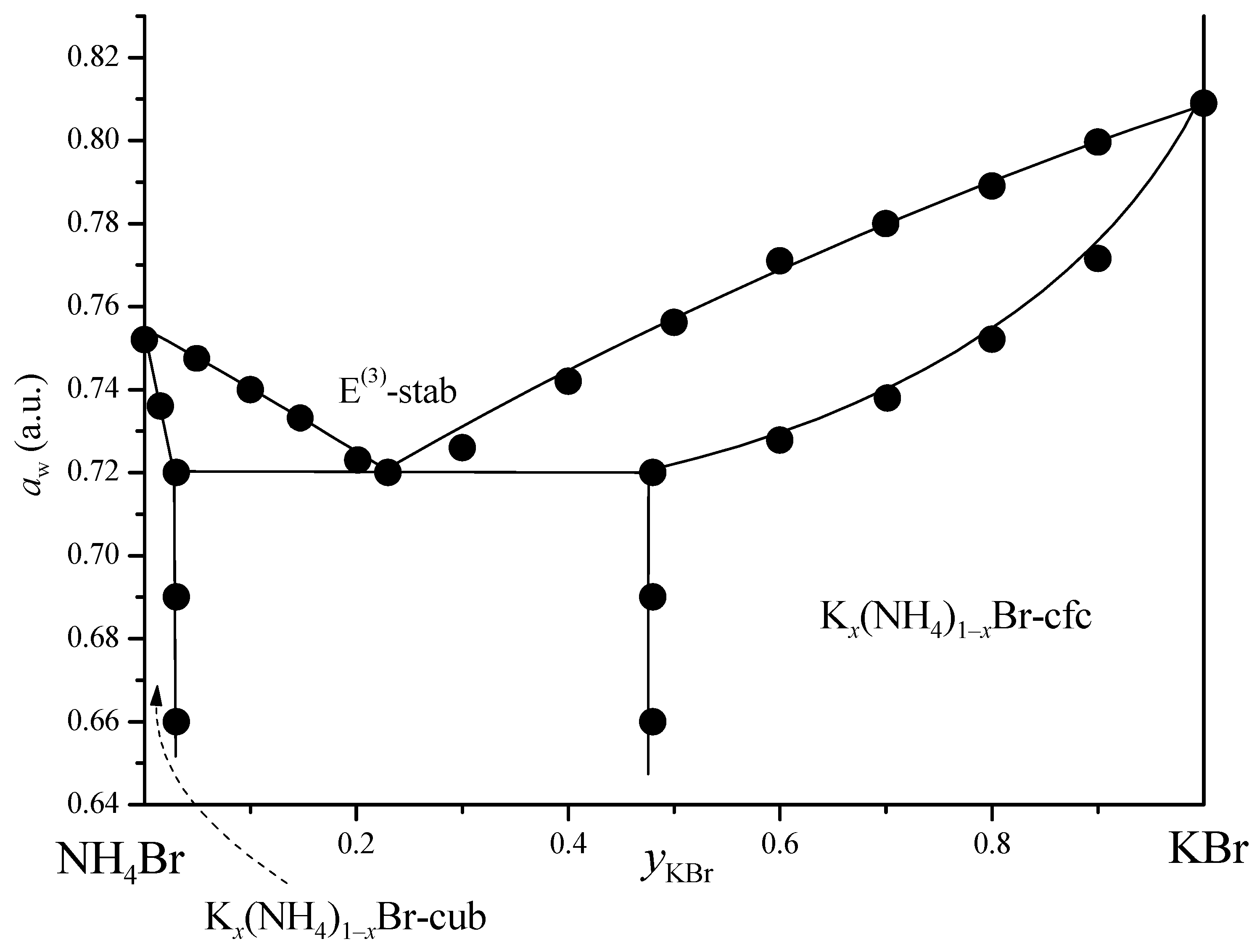
  18. Rumyantsev, A.V.; Charykov, N.A.; Zamoryanskaya, M.V.; Arapov, O.V.; Charykova, M.V.; Shakhmatkin, B.A. Phase Diagrams for the Partial Systems of the Quaternary Reciprocal System K+, NH4+‖Cl, Br–H2O at 25 °C. Russ. J. Inorg. Chem. 2003, 48, 1735–1744. Available online: https://elibrary.ru/item.asp?id=13420521 (accessed on 23 April 2023).
  19. Charykov, N.A.; Arapov, O.V.; Pronkin, A.A.; Charykova, M.V.; Rumyantsev, A.V.; Zamoryanskaya, M.V.; Shakhmatkin, B.A. Topological Isomorphism of Phase Diagrams: The Validity of the Analogues of the Gibbs-Konovalov Laws As Applied to Movement along the Curves of Partial Solvent Activity Extremes. Russ. J. Inorg. Chem. 2005, 50, 93–100. Available online: https://elibrary.ru/item.asp?id=13500150 (accessed on 23 April 2023).
  20. Hamer, W.H.; Wu, Y.-C. Osmotic Coefficients and Mean Activity Coefficients of Uni-univalent Electrolytes in Water at 25 °C. J. Phys. Chem. Ref. Data 1972, 1, 1047–1099. [Google Scholar] [CrossRef]
  21. Robinson, R.A. The activity coefficients of some alkali halides at 25°. Trans. Faraday Soc. 1939, 35, 1217–1220. [Google Scholar] [CrossRef]
  22. McCoy, W.H.; Wallace, W.E. Activity Coefficients in Concentrated Aqueous KCl–KBr Solutions at 25°. J. Am. Chem. Soc. 1956, 78, 1830–1833. [Google Scholar] [CrossRef]
  23. Simanova, S.A.; Shul’ts, M.M. Thermodynamic study of the KBr–NH4Br–H2O system at 25 °C. I. Water activity and activity coefficients of KBr and NH4Br in binary and ternary solutions. Vestn. LGU Ser. (Phys. Chem.) 1966, 4, 75–81. (In Russian) [Google Scholar]
  24. Wishaw, B.F.; Stokes, R.H. The osmotic and activity coefficients of aqueous solutions of ammonium chloride and ammonium nitrate at 25°. Trans. Faraday Soc. 1953, 49, 27–31. [Google Scholar] [CrossRef]
  25. Kirgintsev, A.N.; Luk’yanov, A.V. The study of ternary solutions by the isopiestic method. III. The NaCl–NaNO3–H2O; NaCl–NaBr–H2O; NH4Cl–NH4Br–H2O ternary solutions. Zhurnal Fiz. Khimii 1964, 38, 1603–1605. (In Russian) [Google Scholar]
  26. Shul’ts, M.M.; Simanova, S.A. Activity coefficients of ammonium bromide in aqueous solution at 25 °C. Zhurnal Fiz. Khimii 1966, 40, 462–463. (In Russian) [Google Scholar]
  27. Covington, A.K.; Irish, D.E. Osmotic and activity coefficients of aqueous ammonium bromide solutions at 25 °C. J. Chem. Eng. Data 1972, 17, 175–176. [Google Scholar] [CrossRef]
  28. Cohen-Adad, R.; Lorimer, J.W. Solubility Data Series 47: Alkali Metal and Ammonium Chlorides in Water and Heavy Water (Binary Systems); Pergamon Press: Oxford, UK, 1991; pp. 218–419. Available online: https://srdata.nist.gov/solubility/IUPAC/SDS-47/SDS-47.pdf (accessed on 23 April 2023).
  29. Zdanovskiy, A.B.; Solov’eva, E.F.; Ezrokhi, L.L.; Lyakhovskaya, E.I. Handbook of Experimental Data on Solubility of Salt Systems, Volume 3: Two-Component Systems; Group I Elements and Their Compounds; Khimicheskaya Literatura: Lenengrad, Russia, 1961; p. 2068. (In Russian) [Google Scholar]
  30. Covington, A.K.; Lilley, T.H.; Robinson, R.A. Excess free energies of aqueous mixtures of some alkali metal halide salt pairs. J. Phys. Chem. 1968, 72, 2759–2763. [Google Scholar] [CrossRef]
  31. Staveley, L.A.K.; Davies, N.J.; Fernanda, M.; Silva, P.; Lobo, L.Q. The thermodynamics of mixed crystals of (ammonium chloride + ammonium bromide): IV. The excess Gibbs free energy, excess enthalpy, and excess entropy at the temperature T = 298.15 K and at T = 0. J. Chem. Thermodyn. 1995, 27, 787–799. [Google Scholar] [CrossRef]
  32. Filippov, V.K.; Fedorov, Y.A. Application of Pitzer’s equations to calculation of solubility diagrams of the systems obeying to Zdanovskii’s rule. Dokl. Akad. Nauk SSSR 1983, 273, 393–396. (In Russian) [Google Scholar]
  33. Fock, A. Ueber die Löslichkeit von Mischkrystallen und die Grösse des Krystallmoleküls. Z. Kryst. Mineral. 1897, 28, 337–413. [Google Scholar] [CrossRef]
  34. Touren, C. Solubilité d’un Mélange de Sels Ayant un ion Commun. Comptes Rendus 1900, 130, 1252–1254. Available online: https://gallica.bnf.fr/ark:/12148/bpt6k3086n/f1252.item (accessed on 23 April 2023).
  35. Boeke, H.E. Über das Krystallisationsschema der Chloride, Bromide, Jodide von Natrium, Kalium und Magnesium, sowie über das Vorkommen des Broms und das Fehlen von Jod in den Kalisalzlagerstätten. Z. Kryst. Mineral. 1908, 45, 346–391. [Google Scholar] [CrossRef]
  36. Amadori, M.; Pampanini, G. Sulla capacita degli alogenuri potassici di dare soluzioni solide, in rapporto colla temperatura. Atti Accad. Lincei Ser. 5 1911, 20, 473–480. [Google Scholar]
  37. Nikolaev, V.I. On the equilibria of bromine- and potassium-containing water systems in connection with the industrial use of Solikamsk sylvinites for bromine. Izv. Inst. Fiz.-Khim. Anal. AN SSSR 1935, 7, 135–158. (In Russian) [Google Scholar]
  38. Bergman, A.G.; Vlasov, N.A. Polytherm of the ternary system H2O–KCl–KBr. Dokl. AN SSSR 1942, 36, 64–68. (In Russian) [Google Scholar]
  39. Bergman, A.G.; Vlasov, N.A. Homeomorphism of halogen potassium salts and polytherms of the ternary systems KCl–KBr–H2O, NaCl–NaBr–H2O, NaBr–KBr–H2O, NaCl–KCl–H2O. Izv. Sect. Fiz.-Khim. Anal. AN SSSR 1949, 17, 312–337. (In Russian) [Google Scholar]
  40. Flatt, R.; Burkhardt, G. Untersuchungen über Mischkrystallbildung in Lösungen. II. Die Systeme KCl + NH4Cl + H2O, KBr + NH4Br + H2O, KCl + KBr + H2O und NH4Cl + NH4Br + H2O bei 25°. Helv. Chim. Acta 1944, 27, 1605–1610. [Google Scholar] [CrossRef]
  41. Zdanov, A.K. Equilibria in the system water–potassium chloride–potassium bromide–potassium iodide. Zhurnal Obshsc. Khimii 1948, 18, 554–558. (In Russian) [Google Scholar]
  42. Zdanov, A.K. Equilibria in the system sodium chloride—Sodium bromide—Water at 25°. Uzb. Khimicheskii Zhurnal 1959, 39–44. [Google Scholar]
  43. Durham, G.S.; Rock, E.J.; Frayn, J.S. Solid Solutions of the Alkali Halides. I. The Systems KBr–KCl–H2O, RbBr–RbCl–H2O and RbBr–KBr–H2O at 25°. J. Am. Chem. Soc. 1953, 75, 5792–5794. [Google Scholar] [CrossRef]
  44. Dejewska, B. The Distribution Coefficient of Isomorphous Admixtures for KCl–KBr–H2O, K2SO4–(NH4)2SO4–H2O and KNO3–NH4NO3–H2O Systems at 298 K. Cryst. Res. Technol. 1992, 27, 385–394. [Google Scholar] [CrossRef]
  45. Dejewska, B. Some Physicochemical Parameters of Saturated Ternary Solutions of Systems with Mixed Crystals in their Solid Phase. Cryst. Res. Technol. 1993, 28, 697–705. [Google Scholar] [CrossRef]
  46. Nikl, S.; Nývlt, J. Correlation of solubilities in systems with components forming solid solutions; The system KBr–KCl–H2O. Collect. Czechoslov. Chem. Commun. 1976, 41, 2657–2664. [Google Scholar] [CrossRef]
  47. Dejewska, B.; Szymański, T. The Base of the Computation of Quantitative Changes Running in Technological Processes in the Multicomponent Systems with Mixed Crystals. Cryst. Res. Technol. 1998, 33, 757–765. [Google Scholar] [CrossRef]
  48. Charykov, N.A.; Shvedov, D.N.; Puchkov, L.V.; Korovin, A.V.; Tumanovskii, A.A. Phase Equlibria in the Na+‖Cl, Br–H2O and K+‖Cl, Br–H2O Systems at 25 °C. Zhurnal Prikl. Khimii 1991, 64, 2582–2587. [Google Scholar]
  49. Dejewska, B.; Sędzimir, A. X-ray powder diffraction investigations of solid solutions in the KCl–KBr–H2O system at 298 K. Cryst. Res. Technol. 1989, 24, 1003–1008. [Google Scholar] [CrossRef]
  50. Chmarzyński, A.; Dejewska, B. Enthalpies of crystallisation of equilibrium solid phases occurring in the system KCl−KBr−H2O at 298.15 K. J. Therm. Anal. 1995, 45, 799–804. [Google Scholar] [CrossRef]
  51. McCoy, W.H.; Wallace, W.E. Free Energies and Entropies of Formation of KCl–KBr Solid Solutions at 25°. J. Am. Chem. Soc. 1956, 78, 5995–5998. [Google Scholar] [CrossRef]
  52. Kirgintsev, A.N.; Trushnikova, L.N. Thermodynamics of solid solutions MCl–MBr. Zhurnal Neorg. Khimii 1966, 11, 2331–2339. (In Russian) [Google Scholar]
  53. Kirgintsev, A.N. Essays on the Thermodynamics of Water-Salt Systems; Nauka: Novosibirsk, Russia, 1976; pp. 123–125, 152–160. (In Russian) [Google Scholar]
  54. Königsberger, E. Analysis of Lippmann diagrams: Binary alkali halide systems. Mon. Chem. 1990, 121, 999–1004. [Google Scholar] [CrossRef]
  55. Kirgintsev, A.N.; Visyagina, L.N. Thermodynamics of the NH4Cl–NH4Br solid solutions at 25 °C. Zhurnal Neorg. Khimii 1964, 9, 698–701. (In Russian) [Google Scholar]
  56. Christov, C.; Petrenko, S.; Balarew, C.; Valyashko, V. Calculation of the Gibbs energy of mixing in crystals using Pitzer’s model. J. Solut. Chem. 1994, 23, 795–812. [Google Scholar] [CrossRef]
  57. Biltz, W.; Markus, E. Über Ammoniumcarnallit. Z. Anorg.Chem. 1911, 71, 166–181. [Google Scholar] [CrossRef]
  58. Uyeda, K. On mixed crystals of potassium and ammonium chlorides. In Proceedings of the Original Communications, Eighth International Congress of Applied Chemistry, Washington, DC, USA, and New York, NY, USA, 4–13 September 1912; Section 10b. Volume 22, pp. 235–237. Available online: https://babel.hathitrust.org/cgi/pt?id=inu.30000091326151&view=1up&seq=247 (accessed on 23 April 2023).
  59. Yarlykov, M.M. Equilibrium solubility state of the systems KCl–H2O–NH4Cl and NaCl–H2O–NH4Cl. Zhurnal Prikl. Khimii 1934, 7, 902–905. (In Russian) [Google Scholar]
  60. Hill, A.E.; Loucks, C.M. The Reciprocal Salt-pair (NH4)2SO4 + 2KCl ⇄ K2SO4 + 2NH4Cl in Water and in Ammonia–Water at 25°. J. Am. Chem. Soc. 1937, 59, 2094–2098. [Google Scholar] [CrossRef]
  61. Zhuravlev, E.F.; Kudryashov, S.F. The K+, NH4+‖Cr2O72−, Cl–H2O system. Zhurnal Neorg. Khimii 1964, 9, 1996–2006. (In Russian) [Google Scholar]
  62. Bogoyavlenskii, P.S.; Manannikova, A.S. Study of solubility in the NH4Br–KBr–H2O system. Zhurnal Neorg. Khimii 1961, 6, 977–984. (In Russian) [Google Scholar]
  63. Simanova, S.A.; Shul’ts, M.M. Thermodynamic study of the KBr–NH4Br–H2O system at 25 °C. Vestn. LGU Ser. (Phys. Chem.) 1966, 4, 82–90. (In Russian) [Google Scholar]
  64. Kalinkin, A.M.; Rumyantsev, A.V. Thermodynamics of phase equilibria of the K2SO4 + Rb2SO4 + H2O system at 25 °C. J. Solut. Chem. 1996, 25, 695–709. [Google Scholar] [CrossRef]
  65. Charykov, N.A.; Gur’eva, A.A.; German, V.P.; Keskinov, V.A.; Rumyantsev, A.V.; Semenov, K.N.; Kulenova, N.A.; Sadenova, M.A.; Shushkevich, A.V.; Letenko, D.G.; et al. Solubility in the ternary system GdCl3–TbCl3–H2O water-salt system at 25 °C. Zhurnal Fiz. Khimii 2023, 97, 7. [Google Scholar]
  66. Rumyantsev, A.V.; Gur’eva, A.A.; German, V.P.; Keskinov, V.A.; Charykov, N.A.; Blokhin, A.A.; Kulenova, N.A.; Shaymardanova, B.K.; Sadenova, M.A.; Shushkevich, A.V. Solubility in the ternary system NdCl3–PrCl3–H2O at 25 °C. Zhurnal Fiz. Khimii 2023, 97, 8. [Google Scholar]
  67. Benrath, A.; Neumann, E. Über Mischkristalle in der Vitriolreihe. V. Z. Anorg. Chem. 1939, 242, 70–78. [Google Scholar] [CrossRef]
  68. Soboleva, O.S. Equilibria in the system MgSO4–NiSO4–H2O. Part I. Isotherms of the solubility. Khim. Sbirnik Lvivsk. Univ. 1958, 46, 91–106. (In Ukrainian) [Google Scholar]
  69. Benrath, A.; Triemann, W. Über Mischkristalle in der Vitriolreihe. III. Z. Anorg. Chem. 1934, 217, 347–352. [Google Scholar] [CrossRef]
  70. Rohmer, R. Contribution a l’etude du sulfate de nickel et du sulfate de cobalt. Ann. Chim. (11è Sér.) 1939, 11, 611–725. [Google Scholar]
  71. Shchedrina, A.P.; Krasnova, L.I.; Ozerova, M.I. The FeCl2–MgCl2–H2O system at 40 °C. Zhurnal Neorg. Khimii 1969, 14, 265–267. (In Russian) [Google Scholar]
  72. Shchedrina, A.P.; Krasnova, L.I. The FeCl2–MgCl2–H2O system at 50 °C. Zhurnal Neorg. Khimii 1969, 14, 2194–2196. (In Russian) [Google Scholar]
  73. Shchedrina, A.P.; Krasnova, L.I.; Mel’nichenko, L.M. The FeCl2–MgCl2–H2O system at 60 °C. Zhurnal Neorg. Khimii 1970, 15, 1931–1933. (In Russian) [Google Scholar]
  74. Litvak, A.M.; Charykov, N.A. A new thermodynamic method for calculating melt-solid phase equilibria (using A3B5 systems as an example). Zhurnal Phys. Khimii 1990, 64, 2331–2335. (In Russian) [Google Scholar]
  75. Charykov, N.A.; Litvak, A.M.; Mikhailova, M.P.; Moiseev, K.D.; Yakovlev, Y.P. Solid solution InxGa1–xAsySbzP1–y–z: A new material for infrared optoelectronics. I. Thermodynamic analysis of the conditions for obtaining solid solutions, isoperiodic to InAs and GaSb substrates, by liquid-phase epitaxy. Semiconductors 1997, 31, 344–349. [Google Scholar] [CrossRef]
  76. Grebenyuk, A.M.; Litvak, A.M.; Charykov, N.A.; Puchkov, L.V.; Yakovlev, Y.P.; Klepikov, V.V.; Udovenko, A.G.; Izotova, S.G.; Charykova, M.V.; Zubkova, M.Y. On the Calculation of Melt-Solid Phase Equilibria in the Pb–InAs–GaAs–InSb–GaSb System. Zhurnal Neorg. Khimii 1999, 44, 113–114. (In Russian) [Google Scholar]
  77. Flatt, R.; Burkhardt, G. Untersuchungen über Mischkrystallbildung in Lösungen. III. Die Bildung ternärer Mischkrystalle im System K∙ + NH4∙ + Cl′ + Br′ + H2O. Helv. Chim. Acta 1944, 27, 1611–1621. [Google Scholar] [CrossRef]
Figure 1. Diagram of solubility of the ternary system NaCl–CdCl2–H2O at 25 °C [3]. E is ternary eutonics, D is ternary distonics.
Processes 11 01405 g001
Figure 2. Solubility diagram of the Na + , Cd 2 + | | Cl , SO 4 2 —quaternary reciprocal system at 25 °C [3]. The thin dashed and solid lines are isopotentials of water in the crystallization field of the ternary compound. The end of the arrow points to the point of the compound and simultaneously to the maximum activity of water.
Processes 11 01405 g002
Figure 3. (a) Calculated values of excess Gibbs energy of solid solution formation in experimental points (open signs) and their approximation by regular model (solid lines) and subregular model (dotted lines) in the systems K + , NH 4 + | | Br H 2 O (left) and K + | | Cl , Br H 2 O (right) at 25 °C. (b) Calculated values of excess Gibbs energy of solid solution formation in experimental points (open signs) and their approximation by regular model (solid lines) in the systems K + , NH 4 + | | Cl H 2 O (left) and NH 4 + | | Cl , Br H 2 O (right) at 25 °C.
Processes 11 01405 g003aProcesses 11 01405 g003b
Figure 4. Experimental (open signs) and calculated (solid lines) data on the composition of saturated solutions in ternary systems K + , NH 4 + | | Cl H 2 O , K + , NH 4 + | | Br H 2 O , K + | | Cl , Br H 2 O , NH 4 + | | Cl , Br H 2 O at 25 °C (in salt molalities). Data falling out of the general set: a number of triangles with a base on the right [33], stars [44,45], a few pentagons [61].
Processes 11 01405 g004
Figure 5. (a) The systems K + , NH 4 + | | Br H 2 O (left) and K + | | Cl , Br H 2 O (right) at 25 °C: experimental (open signs) and calculated (solid lines) data on the distribution of salt components between liquid and solid solutions in solvent-free concentration space (Janecke indexes). (b) The systems K + , NH 4 + | | Cl H 2 O (left) and NH 4 + | | Cl , Br H 2 O (right) at 25 °C: experimental (open signs) and calculated (solid lines) data on the distribution of salt components between liquid and solid solutions in solvent-free concentration space (Janecke indexes).
Processes 11 01405 g005aProcesses 11 01405 g005b
Figure 6. Diagram of solubility as water activity vs. Janecke index of the TbCl3–GdCl3–H2O system at 25 °C under formation of the Tb x Gd 1 x Cl 3 · 6 H 2 O solid solutions.
Processes 11 01405 g006
Figure 7. Solubility diagram of water activity vs. Janecke index of the KCl–KBr–H2O system at 25 °C. Solid points correspond to the formation of stable solid solutions on the base of face-centered (cfc) lattice, while open circles correspond to metastable cubic (cub) solution formation. Hereafter, A(3) is alyotrope point.
Processes 11 01405 g007
Figure 8. Solubility diagram of water activity vs. Janecke index of the NH4Cl–NH4Br–H2O system at 25 °C. Solid points correspond to the formation of stable solid solutions on the base of cubic (cub) lattice, while open circles correspond to the metastable face-centered (cfc) solution formation.
Processes 11 01405 g008
Figure 9. Solubility diagram of water activity vs. Janecke index of the KCl NH 4 Cl H 2 O system at 25 °C. All solid solutions have cubic syngony (cub). Solid points correspond to stable part of diagram; open cycles respond metastable one. Hereafter, E(3) is ternary eutonics.
Processes 11 01405 g009
Figure 10. Solubility diagram of water activity vs. Janecke index of the KBr NH 4 Br H 2 O system at 25 °C. All solid solutions have cubic syngony (cub). Solid points correspond to stable part of diagram; open cycles respond metastable one.
Processes 11 01405 g010
Figure 11. Solubility diagram of water activity vs. Janecke index of the KCl NH 4 Cl H 2 O system at 25 °C.
Processes 11 01405 g011
Figure 12. Solubility diagram of water activity vs. Janecke index of the KBr NH 4 Br H 2 O system at 25 °C.
Processes 11 01405 g012
Figure 13. Solubility diagram of water activity vs. Janecke index of the NdCl3–PrCl3–H2O system at 25 °C [66]. Solid solutions are Pr x Nd 1 x Cl 3 · 7 H 2 O and Pr x Nd 1 x Cl 3 · 6 H 2 O .
Processes 11 01405 g013
Figure 14. Basic schemes of diagram of solubility of the CA   C A H 2 O ternary system with the dehydration of solid solution. C X   C 1 X A · Q 1 H 2 O C X   C 1 X A · Q 2 H 2 O + Q 1 Q 2 H 2 O   ( Q 1 > Q 2 ) . Waters activities of dehydration of binary crystal hydrates are a W d s CA · Q 1 H 2 O and a W d s C A · Q 1 H 2 O .
Processes 11 01405 g014
Figure 15. Scheme of diagram of solubility in ternary system with the formation of solid solutions on the base of ternary compound (double salt).
Processes 11 01405 g015
Figure 16. Solubility diagram of the system K + , NH 4 + | | Cl , Br H 2 O at 25 °C in solvent-free concentration space (Janecke indexes). Gray circles denote experimental data [77], and straight segments are tie lines. The minimum of water activity is designated by black points.
Processes 11 01405 g016
Figure 17. Isoconcentrates of potassium ( Y K , “vertical” thin curves) and chlorine ( Y Cl , “horizontal” dotted curves) in the liquid phase of the K + , NH 4 + | | Cl , Br H 2 O system at 25 °C.
Processes 11 01405 g017
Figure 18. The K + , NH 4 + | | Cl , Br H 2 O system at 25 °C: water isoactivity lines (thin solid curves) in the variables of liquid phase. The dotted curves ( A 1 3 A 4 and A 4 A 2 3 ) indicate the lines of incomplete alyotropes.
Processes 11 01405 g018
Figure 19. Fragment of solubility diagram of the K + , NH 4 + | | Cl , Br H 2 O system at 25 °C: water isoactivity lines in the field of crystallization of the K x NH 4 1 x Cl y   Br 1 y c f c solid solutions in the concentration variables of the latter. The designations are the same as in Figure 18.
Processes 11 01405 g019
Figure 20. Fragment of solubility diagram of the K + , NH 4 + | | Cl , Br H 2 O system at 25 °C: water isoactivity lines in the field of crystallization of the K x NH 4 1 x Cl y   Br 1 y c u b solid solutions in the concentration variables of the latter. The designations are the same as in Figure 18.
Processes 11 01405 g020
Figure 21. Isotherm–isobars of open evaporation–crystallization in the field of crystallization of the K x NH 4   1 x Cl y   Br 1 y c f c solid solutions in the K + , NH 4 + | | Cl , Br H 2 O system at 25 °C are solid curves. Other designations are as above.
Processes 11 01405 g021
Figure 22. Liquidus (upper) and solidus (bottom) curves when moving along the open evaporation–crystallization curve from the point of ternary alyotrope A 2 3 to the point of incomplete quaternary alyotrope A 4 in the field of crystallization of the K x NH 4   1 x Cl y   Br 1 y c f c solid solutions in the K + , NH 4 + | | Cl , Br H 2 O system at 25 °C.
Processes 11 01405 g022
Figure 23. Liquidus (upper) and solidus (bottom) curves when moving along the open evaporation–crystallization curve to the point of incomplete quaternary alyotrope A 4 in the field of crystallization of the K x NH 4   1 x Cl y   Br 1 y c f c solid solutions in the K + , NH 4 + | | Cl , Br H 2 O system at 25 °C.
Processes 11 01405 g023
Figure 24. Incomplete extrema curves in the field of crystallization of the K x NH 4   1 x Cl y   Br 1 y c f c and K x NH 4   1 x Cl y   Br 1 y c u b solid solutions in the system K + , NH 4 + | | Cl , Br H 2 O at 25 °C are dashed lines. The dotted straight lines indicate the concentration sections.
Processes 11 01405 g024
Figure 25. Liquidus and solidus curves when moving along incomplete extrema curve in the fields of crystallization of the K x NH 4   1 x Cl y   Br 1 y c f c and K x NH 4   1 x Cl y   Br 1 y c u b solid solutions in the system K + , NH 4 + | | Cl , Br H 2 O at 25 °C.
Processes 11 01405 g025
Figure 26. Metastable liquidus and solidus curves when moving along incomplete extrema curve in the field of crystallization of the K x NH 4   1 x Cl y   Br 1 y c f c solid solutions in the system K + , NH 4 + | | Cl , Br H 2 O at 25 °C.
Processes 11 01405 g026
Figure 27. Metastable liquidus and solidus curves when moving along incomplete extrema curve in the field of crystallization of the K x NH 4   1 x Cl y   Br 1 y c u b solid solutions in the system K + , NH 4 + | | Cl , Br H 2 O at 25 °C.
Processes 11 01405 g027
Figure 28. Curves of thermodynamic simplification t s K + , NH 4 + in solubility diagram of the quaternary reciprocal system K + , NH 4 + | | Cl , Br H 2 O at 25 °C in the variables of liquid phase (solid lines) and of the K x NH 4 1 x Cl y   Br 1 y c f c solid solutions (dotted lines).
Processes 11 01405 g028
Figure 29. Curves of thermodynamic simplification t s Cl , Br in solubility diagram of the quaternary reciprocal system K + , NH 4 + | | Cl , Br H 2 O at 25 °C in the variables of liquid phase (solid lines) and of the K x NH 4 1 x Cl y   Br 1 y c f c solid solutions (dotted lines).
Processes 11 01405 g029
Figure 30. Metastable liquidus and solidus curves when moving along a thermodynamic simplification curve in the field of crystallization of the K x NH 4   1 x Cl y   Br 1 y c f c solid solutions in the system K + , NH 4 + | | Cl , Br H 2 O at 25 °C. Incomplete quaternary pseudoalyotrope is denoted as A(4).
Processes 11 01405 g030
Figure 31. Metastable liquidus and solidus curves when moving along a thermodynamic simplification curve in the field of crystallization of the K x NH 4   1 x Cl y   Br 1 y c f c solid solutions in the system K + , NH 4 + | | Cl , Br H 2 O at 25 °C. Incomplete quaternary pseudoalyotrope is denoted as A(4).
Processes 11 01405 g031
Table 1. Binary parameters of Pitzer’s equations in the NH 4 + ,   K + | | Cl , Br H 2 O quaternary system at 25 °C.
SystemBinary Parameter Values
β 0 β 1 β 2 C φ α 1 α 2
NH 4 Cl H 2 O 0.052010.1922−0.003012.0
KCl H 2 O 0.046320.2222−0.0003972.0
NH 4 Br H 2 O 0.042400.064540.0981−0.002222.01.0
KBr H 2 O 0.025430.2307−0.001562.0
Table 2. Solubility and thermodynamic potentials of binary solid phases in the NH 4 + ,   K + | | Cl , Br H 2 O quaternary system at 25 °C.
Solid CompositionSyngony aSolubility, m(s), mole/kg H2Oln SP
KClcfc4.769 b2.064
cub e6.2 ± 1.22.7 ± 0.5
KBrcfc5.72 c2.595
cub e6.5 ± 1.02.9 ± 0.4
NH4Clcub7.393 b2.853
cfc e9.3 ± 0.93.3 ± 0.2
NH4Brcub7.993 d3.115
cfc e9.6 ± 0.33.47 ± 0.07
a Hereafter: cfc—cubic face-centered lattice, cub—cubic lattice. b Corresponding values at 25 °C (26.23% and 28.34%) are recommended in [28]. c Value at 25 °C (40.5%) is recommended in [29]. d Average value at 25 °C from the data of 12 articles (43.91 ± 0.07%). e The solid phase of this syngony is metastable at 25 °C.
Table 3. Parameters of regular and subregular models for solid solutions at 25 °C.
System * α 0 ,   kJ / mol α 1 ,   kJ / mol System * α 0 ,   kJ / mol α 1 ,   kJ / mol
NH 4 Cl KCl   c u b 7.7 ± 1.8 NH 4 Cl KCl   c f c 3.8 ± 0.2
NH 4 Br KBr c u b 8.5 ± 1.2 NH 4 Br KBr c f c 2.9 ± 0.3
KCl
KBr c u b
3.6 ± 0.5 KCl
KBr c f c
3.64 ± 0.05
3.63 ± 0.06
0.5 ± 0.1
NH 4 Cl NH 4 Br c u b 3.8 ± 0.1 NH 4 Cl NH 4 Br c f c 3.7 ± 0.7
* cub—cubic lattice, cfc—cubic face-centered lattice.
Disclaimer/Publisher’s Note: The statements, opinions and data contained in all publications are solely those of the individual author(s) and contributor(s) and not of MDPI and/or the editor(s). MDPI and/or the editor(s) disclaim responsibility for any injury to people or property resulting from any ideas, methods, instructions or products referred to in the content.

