Some Logarithmic Intuitionistic Fuzzy Einstein Aggregation Operators under Confidence Level

Abstract

The objective of this paper is to introduce some new logarithm operational laws for intuitionistic fuzzy sets. Some structure properties have been developed and based on these, various aggregation operators, namely confidence logarithmic intuitionistic fuzzy Einstein weighted geometric (CLIFEWG) operator, confidence logarithmic intuitionistic fuzzy Einstein ordered weighted geometric (CLIFEOWG) operator, confidence logarithmic intuitionistic fuzzy Einstein hybrid geometric (CLIFEHG) operator, confidence logarithmic intuitionistic fuzzy Einstein weighted averaging (CLIFEWA) operator, confidence logarithmic intuitionistic fuzzy Einstein ordered weighted averaging (CLIFEOWA) operator, confidence logarithmic intuitionistic fuzzy Einstein hybrid averaging (CLIFEHA) operator have been presented. To show the validity and the superiority of the proposed operators, we compared these methods with the existing methods and concluded from the comparison and sensitivity analysis our proposed techniques are more effective.

1. Introduction

Multiple Decision-making plays a significant role in several disciplines, such as medicine, social sciences, engineering, business management, computer science, automotive industries, management science, information technology, robotics, and several other disciplines of science and technology. Decision-making is one of the appropriate processes to find the more suitable alternative from all the possible alternatives. Traditionally, it has been generally assumed that all the information that accesses the alternative in terms of criteria and their corresponding weights are expressed in the form of crisp numbers. But most of the decisions in real-life situations are taken in an environment where the goals and constraints are generally imprecise or vague in nature. In order to handle the uncertainties, vagueness, and fuzziness, there are several theories, namely soft sets theory [1], rough sets theory [2], and fuzzy sets theory [3] are developed to handle imprecision and uncertainty that occurs in practically all the real-life problems.

All of these theories have their own applications, but Zadeh’s fuzzy set is a noteworthy and mostly useable among them in several cases of uncertainties including clustering, pattern recognition, networking, decision making problems and some other fields. Zadeh’s fuzzy set can be defined as let $Ü$ be a universal set, then fuzzy set $X$ can be written as: $X=\left\{Ó,{\eta }_X\left(Ó\right)|Ó\in Ü\right\}$, where $\eta$ be a mapping from $Ü$ to the closed interval and called the degree of membership function. Hence, the fuzzy set allows us to describe only the membership degree means the degree of satisfaction of an object numerically, and not provide any information about the non-membership degree means the degree of dissatisfaction. For example, if an element’s satisfaction is $0.4$, then its dissatisfaction should be calculated as $1-0.4=0.6$. Thus, scholars and decision makers have not considered dissatisfaction independently in the fuzzy set.

Later on, Atanassov [4] introduced intuitionistic fuzzy sets (IFSs) by presenting each element in the form order, such as $\left(\eta ,¢\right)$, where $\eta$, $¢$ stand for membership degree (MD) and non-membership degree (NMD) with the condition $0\prec \eta +¢\le 1$. Atanassov and Gargov [5] developed interval-valued intuitionistic fuzzy sets (IVIFSs) by presenting each element in the form of $\left(\left[c,\eta \right],\left[d,¢\right]\right)$, where $\left[c,\eta \right]$ and $\left[d,¢\right]$ stands for membership degree (MD) and non-membership degree (NMD) with condition, such as $0\prec \eta +¢\le 1$.

One of the most important tools is aggregation operators. Yager and Kacprzyk [6] developed several basic roles based on intuitionistic fuzzy numbers. Yager [7], Xu and Yager [8], Xu [9] respectively introduced the OWA operator, IFHG operator, IFOWG operator, IFWG operator, IFHA operator, IFOWA operator, and IFWA operator, and presented their advantages in our daily life problems. Ye [10,11] presented the notion of accuracy under environments, such that intuitionistic fuzzy numbers and interval-valued intuitionistic fuzzy numbers. Wang and Liu [12,13] and Zhao and Wei [14] presented numerous new methods using Einstein’s operation laws, namely IFEWG operator, IFEOWG operator, IFEWA operator, IFEOWA operator, IFEHA operator and IFEHG operators and their structural properties and applications. Xu et al. [15] presented the idea of Einstein Choquet integral using intuitionistic fuzzy numbers under Einstein operations. Many generalized novel methods have been presented by Garg in [16,17,18] introduced the accuracy and score function for interval-valued intuitionistic fuzzy numbers. Some new related methods are found in [19,20,21]. Yu and Shi [22], Garg et al. [23], Dahlman et al. [24] and Kumar and Garg [25] presented several new methods and apply them to group decision making. Gou et al. [26], Rahman et al. [27], Jamil et al. [28], introduced generalized operators using intuitionistic fuzzy sets and interval-valued intuitionistic fuzzy sets. Some related researches are found in [29,30,31]. Atanassov et al. [32] introduced a generalized net model for decision-making, presented advanced fuzzy logic, and applied them to group decision-making problems. Some related works are found in [33,34,35,36,37,38,39].

Li and Wei [40] introduced logarithmic aggregation operators based on intuitionistic fuzzy numbers and proposed many aggregation operators, namely LIFWG operator, LIFOWG operator, LIFWA operator, LIFOWA operator, and their applications. Rahman [41] introduced several new logarithmic approaches using Einstein t-norm and t-conorm and applied them on decision-making problem.

In all of the above methods, we found that all researchers checked their decision and that all of the decision-makers are surely specialists about the objects information. However, in daily life problems this is sometimes fulfilled. Therefor Ma and Zeng [42] and Yu [43,44] introduced the notion of confidence level, and settled several methods, namely the CIFWG operator, the CIFOWG operator, the CIFWA operator, the CIFOWA operator, the CIFEWA operator, the CIFEOWA operator, the CIFEWG operator, the CIFEOWG operator, the CIFHA operator respectively. Rahman [45] presented several Trapezoidal intuitionistic Fuzzy Einstein aggregation operators under confidence level.

Motivated by the methods defined in [43,44], where the authors introduced the concept of confidence level and develop several aggregation operators based on algebraic operational laws and Einstein operational laws. But in this paper, we combine the idea of confidence level with logarithmic operational laws and developed several methods, namely CLIFEWA operator, CLIFEOWA operator, CLIFEHA operator, CLIFEWG operator, CLIFEOWG operator, CLIFEHG operator along with examples and applied them on decision-making. To develop the above stated operators we investigated some of their structure properties.

The contributions of the paper are stated as:

(i)

To present logarithmic laws using intuitionistic fuzzy numbers.

(ii)

To present the aggregation operators based on Einstein t-norm and t-conorm, such as CLIFEWG operator, CLIFEOWG operator, CLIFEHG operator, CLIFEWA operator, CLIFEOWA operator, CLIFEHA operator.

(iii)

To show the efficiency of the novel operators, a decision making problem is considered.

The following paper is planned as: Section 2 presents fundamental definitions and logarithmic operational laws. In Section 3 different operators under intuitionistic fuzzy environment. Section 4 includes emergency decision-making model under the novel approaches with an illustrative example. Section 5 presents comparative and sensitive analysis. Section 6 presents limitation and conclusion.

2. Models and Method

In this section, some basic definitions and results related to IFSs and IFNs on the universal set $Ü$ have been discussed.

Definition 1 [4].

Let $X$ be an intuitionistic fuzzy set defined on a universal set $Ü$ as: $X=\left\{\langle Ó,{\eta }_X\left(Ó\right),{¢}_X\left(Ó\right)\rangle |Ó\in Ü\right\}$, where $\eta :Ü\to \left[0,1\right]$ and $¢:Ü\to \left[0,1\right]$ defines the degree of membership function and the degree non-membership function of the element $Ó\in Ü$ to $X$ respectively with condition, such as $0\prec \eta +¢\le 1$.

Definition 2 [4].

Let $\mu =\left(\eta ,¢\right)$ be an intuitionistic fuzzy number, then its score function, accuracy degree can be defined as: $s\left(\mu \right)=\eta -¢$ and $h\left(\mu \right)=\eta +¢$ with conditions, such as $s\left(\mu \right)\in [-1,1]$ and $h\left(\mu \right)\in [0,1]$ respectively.

Definition 3 [4].

Let ${\mu }_1=\left({\eta }_1,{¢}_1\right)$, and ${\mu }_2=\left({\eta }_2,{¢}_2\right)$ are two intuitionistic fuzzy numbers, then

• If, $s\left({\mu }_1\right)\prec s\left({\mu }_2\right)$, then ${\mu }_1\prec {\mu }_2$
• If, $s\left({\mu }_2\right)\prec s\left({\mu }_1\right)$, then ${\mu }_2\prec {\mu }_1$
• If, $s\left({\mu }_1\right)=s\left({\mu }_2\right)$, then the following cases hold:

  (i) 

  If, $h\left({\mu }_1\right)\prec h\left({\mu }_2\right)$, then ${\mu }_1\prec {\mu }_2$

  (ii) 

  If, $h\left({\mu }_2\right)\prec h\left({\mu }_1\right)$, then ${\mu }_2\prec {\mu }_1$

  (iii) 

  If, $s\left({\mu }_1\right)=s\left({\mu }_2\right)$, then ${\mu }_1={\mu }_2$

Definition 4 [8].

Let $\mu =\left(\eta ,¢\right)$, ${\mu }_1=\left({\eta }_1,{¢}_1\right)$, ${\mu }_2=\left({\eta }_2,{¢}_2\right)$ are three intuitionistic fuzzy numbers, and a real number $ü\succ 0$, then

(i) 

${\mu }_1\oplus {\mu }_2=\left(\frac{{\eta }_1+{\eta }_2}{1+{\eta }_1{\eta }_2},\frac{{¢}_1{¢}_2}{1+\left(1-{¢}_1\right)\left(1-{¢}_2\right)}\right)$

(ii) 

${\mu }_1\otimes {\mu }_2=\left(\frac{{\eta }_1{\eta }_2}{1+\left(1-{\eta }_1\right)\left(1-{\eta }_2\right)},\frac{{¢}_1+{¢}_2}{1+{¢}_1{¢}_2}\right)$

(iii) 

$ü\left(\mu \right)=\left(\frac{{\left(1+\eta \right)}^{ü}-{\left(1-\eta \right)}^{ü}}{{\left(1+\eta \right)}^{ü}+{\left(1-\eta \right)}^{ü}},\frac{2{(¢)}^{ü}}{{\left(2-¢\right)}^{ü}+{(¢)}^{ü}}\right)$

(iv) 

${\left(\mu \right)}^{ü}=\left(\frac{2{\eta }^{ü}}{{\left(2-\eta \right)}^{ü}+{\eta }^{ü}},\frac{{\left(1+¢\right)}^{ü}-{\left(1-¢\right)}^{ü}}{{\left(1+¢\right)}^{ü}+{\left(1-¢\right)}^{ü}}\right)$

(v) 

${\left(\alpha \right)}^{\mu }=\{\begin{array}{lll}{\left(\alpha \right)}^{1-\eta },1-{\left(\alpha \right)}^{¢}& & \alpha \in \left(0,1\right)\\ {\left(\frac{1}{\alpha }\right)}^{1-\eta },1-{\left(\frac{1}{\alpha }\right)}^{¢}& & \alpha \ge 1\end{array}$

(vi) 

${\mu }_1\cup {\mu }_2=\left(\max \left\{{\eta }_1,{\eta }_2\right\},\min \left\{{¢}_1,{¢}_2\right\}\right)$

(vii) 

${\mu }_1\cap {\mu }_2=\left(\min \left\{{\eta }_1,{\eta }_2\right\},\max \left\{{¢}_1,{¢}_2\right\}\right)$

(viii) 

${\mu }^c=\left(¢,\eta \right)$

(ix) 

${\mu }_1\le {\mu }_2$, this means that ${\eta }_1\le {\eta }_2$ and ${¢}_2\le {¢}_1$

(x) 

${\mu }_1={\mu }_2$, this means that ${\eta }_1={\eta }_2$ and ${¢}_2={¢}_1$

Definition 5 [8].

Let $Ü$ be a universal set and $X=\left\{\langle Ó,{\eta }_X\left(Ó\right),{¢}_X\left(Ó\right)\rangle |Ó\in Ü\right\}$ be an intuitionistic fuzzy set, then logarithmic operational laws of IFS $X$ can be defined as: ${\log }_{\alpha }X=\left\{\langle Ó,1-{\log }_{\alpha }{\eta }_X\left(Ó\right),{\log }_{\alpha }\left(1-{¢}_X\left(Ó\right)\right)\rangle |Ó\in Ü\right\}$ with $\alpha \ne 1$ and $0\prec \alpha \le \eta \le 1$.

It can be proved that ${\log }_{\alpha }X$ is also an IFS. By the definition of IFS the membership function and the non-membership function of $X$ satisfy the conditions: ${\eta }_X:Ü\to \left[0,1\right],\forall Ó\in Ü\to {\eta }_X\in \left[0,1\right]$, ${¢}_X:Ü\to \left[0,1\right],\forall Ó\in Ü\to {¢}_X\in \left[0,1\right]$ and $0\le {\eta }_X\left(Ó\right)+{¢}_X\left(Ó\right)\le 1$, $Ó\in Ü$. So ${\eta }_X\left(Ó\right)\le 1-{¢}_X\left(Ó\right)$ and $0\le 1-{¢}_X\left(Ó\right)\le 1$. $0\prec \alpha \le \eta \le 1$ and $\alpha \ne 1$, then the membership function:

• $1-{\log }_{\alpha }{\eta }_X:Ü\to \left[0,1\right],\forall Ó\in Ü\to 1-{\log }_{\alpha }{\eta }_X\left(Ó\right)\in \left[0,1\right]$, the non-membership function:
• ${\log }_{\alpha }\left(1-{¢}_X\right):Ü\to \left[0,1\right],\forall Ó\in Ü\to {\log }_{\alpha }\left(1-{¢}_X\right)\in \left[0,1\right]$, and the indeterminacy function:
• $0\le 1-\left(1-{\log }_{\alpha }{\eta }_X\left(Ó\right)\right)+{\log }_{\alpha }\left(1-{¢}_X\left(Ó\right)\right)\le 1,Ó\in Ü$. Thus, ${\log }_{\alpha }X=\left\{\langle Ó,1-{\log }_{\alpha }{\eta }_X\left(Ó\right),{\log }_{\alpha }\left(1-{¢}_X\left(Ó\right)\right)\rangle |Ó\in Ü\right\}$, $\left(0\prec \alpha \le \eta \le 1,\alpha \ne 1\right)$ is an IFS.

Definition 6 [8].

Let $\mu =\left(\eta ,¢\right)$ be an IFN. If ${\log }_{\alpha }X=\left(1-{\log }_{\alpha }\eta ,{\log }_{\alpha }\left(1-¢\right)\right)$, where $0\prec \alpha \le \eta \le 1$ and $\alpha \ne 1$. The function ${\log }_{\alpha }X$ is called a logarithmic operator, and the value ${\log }_{\alpha }X$ is called a logarithmic IFN (Log-IFN).

It can be proved that ${\log }_{\alpha }X$ is also IFN. Let $0\prec \alpha \le \eta \le 1,\alpha \ne 1$, by the definition of IFN, we have $0\prec \eta \le 1$, $0\le ¢\le 1$ and $0\prec \eta +¢\le 1$. It can be written as: $0\prec \eta \le 1-¢$, then $0\le 1-{\log }_{\alpha }\eta \le 1$, $0\le {\log }_{\alpha }\left(1-¢\right)\le 1$ and $0\le 1-{\log }_{\alpha }+{\log }_{\alpha }\left(1-¢\right)\le 1$. So ${\log }_{\alpha }X=\left(1-{\log }_{\alpha }\eta ,{\log }_{\alpha }\left(1-¢\right)\right)$ is also IFN.

Theorem 1.

Let $\mu =\left(\eta ,¢\right)$ be an IFN with $\alpha \ne 1$, $0\prec \alpha \le \min \left\{\eta ,\left(1-¢\right)\right\}\le 1$, then ${\left(\alpha \right)}^{{\log }_{\alpha }\mu }=\mu$.

Proof. 

Since, we have

$$\begin{array}{ll}{\left(\alpha \right)}^{{\log }_{\alpha }\mu }& =\left({\alpha }^{1-\left(1-{\log }_{\alpha }\left\{\frac{\left(1+\eta \right)-\left(1-\eta \right)}{\left(1+\eta \right)+\left(1-\eta \right)}\right\}\right)},1-{\alpha }^{{\log }_{\alpha }\left\{\frac{1-¢}{\left(2+¢\right)-\left(1+¢\right)}\right\}}\right)\\ & =\left({\alpha }^{1-1+{\log }_{\yen }\left\{\frac{\left(1+\eta \right)-\left(1-\eta \right)}{\left(1+\eta \right)+\left(1-\eta \right)}\right\}},1-{\alpha }^{{\log }_{\yen }\left\{\frac{1-¢}{\left(2+¢\right)-\left(1+¢\right)}\right\}}\right)\\ & =\left(\frac{\left(1+\eta \right)-\left(1-\eta \right)}{\left(1+\eta \right)+\left(1-\eta \right)},1-\frac{1-¢}{\left(2+¢\right)-\left(1+¢\right)}\right)=\left(\eta ,¢\right)=\mu \end{array}$$

Thus, the proof is completed. □

Theorem 2.

Let $\mu =\left(\eta ,¢\right)$ with $\alpha \ne 1$, $0\prec \alpha \le \min \left\{\eta ,\left(1-¢\right)\right\}\le 1$, then ${\left(\alpha \right)}^{{\log }_{\alpha }\mu }=\mu$.

Proof. 

As, we know that

$$\begin{array}{ll}{\log }_{\alpha }{\alpha }^{\mu }& ={\log }_{\alpha }\left({\alpha }^{1-\left(\frac{\left(1+\eta \right)-\left(1-\eta \right)}{\left(1+\eta \right)+\left(1-\eta \right)}\right)},1-{\alpha }^{\frac{1-¢}{\left(2+¢\right)-\left(1+¢\right)}}\right)\\ & =\left(1-{\log }_{\alpha }{\alpha }^{1-\left(\frac{\left(1+\eta \right)-\left(1-\eta \right)}{\left(1+\eta \right)+\left(1-\eta \right)}\right)},{\log }_{\alpha }\left(1-\left(1-{\yen }^{\frac{1-¢}{\left(2+¢\right)-\left(1+¢\right)}}\right)\right)\right)\\ & =\left(1-1+\left(\frac{\left(1+\eta \right)-\left(1-\eta \right)}{\left(1+\eta \right)+\left(1-\eta \right)}\right),\frac{1-¢}{\left(2+¢\right)-\left(1+¢\right)}\right)=\left(\eta ,¢\right)=\mu \end{array}$$

Thus, the proof is completed. □

Theorem 3.

Let ${\mu }_j=\left({\eta }_j,{¢}_j\right)\left(j\le 3\right)$ with ${\alpha }_j\ne 1$, $0\prec {\alpha }_j\le \min \left\{{\eta }_j,\left(1-{¢}_j\right)\right\}\le 1$, then

(i) 

${\log }_{\alpha }{\mu }_1\cup {\log }_{\alpha }{\mu }_2={\log }_{\alpha }{\mu }_2\cup {\log }_{\alpha }{\mu }_1$

(ii) 

${\log }_{\alpha }{\mu }_1\cap {\log }_{\alpha }{\mu }_2={\log }_{\alpha }{\mu }_2\cap {\log }_{\alpha }{\mu }_1$

(iii) 

${\log }_{\alpha }\left({\mu }_1\cup {\mu }_2\right)\cap {\log }_{\alpha }{\mu }_2={\log }_{\alpha }{\mu }_2$

(iv) 

${\log }_{\alpha }\left({\mu }_1\cap {\mu }_2\right)\cup {\log }_{\alpha }{\mu }_2={\log }_{\alpha }{\mu }_2$

(v) 

${\log }_{\alpha }\left({\mu }_1\cup {\mu }_2\right)\cap {\log }_{\alpha }{\mu }_3={\log }_{\alpha }\left({\mu }_1\cap {\mu }_3\right)\cup {\log }_{\alpha }\left({\mu }_2\cap {\mu }_3\right)$

(vi) 

${\log }_{\alpha }\left({\mu }_1\cap {\mu }_2\right)\cup {\log }_{\alpha }{\mu }_3={\log }_{\alpha }\left({\mu }_1\cup {\mu }_3\right)\cap {\log }_{\alpha }\left({\mu }_2\cup {\mu }_3\right)$

(vii) 

${\log }_{\alpha }\left({\mu }_1\cup {\mu }_2\right)\oplus {\log }_{\alpha }{\mu }_3={\log }_{\alpha }\left({\mu }_1\oplus {\mu }_3\right)\cup {\log }_{\alpha }\left({\mu }_2\oplus {\mu }_3\right)$

(viii) 

${\log }_{\alpha }\left({\mu }_1\cup {\mu }_2\right)\oplus {\log }_{\alpha }{\mu }_3={\log }_{\alpha }\left({\mu }_1\oplus {\mu }_3\right)\cup {\log }_{\alpha }\left({\mu }_2\oplus {\mu }_3\right)$

(ix) 

${\log }_{\alpha }\left({\mu }_1\cap {\mu }_2\right)\oplus {\log }_{\alpha }{\mu }_3={\log }_{\alpha }\left({\mu }_1\oplus {\mu }_3\right)\cap {\log }_{\alpha }\left({\mu }_2\oplus {\mu }_3\right)$

(x) 

${\log }_{\alpha }\left({\mu }_1\cup {\mu }_2\right)\otimes {\log }_{\alpha }{\mu }_3={\log }_{\alpha }\left({\mu }_1\otimes {\mu }_3\right)\cup {\log }_{\alpha }\left({\mu }_2\otimes {\mu }_3\right)$

(xi) 

${\log }_{\alpha }\left({\mu }_1\cap {\mu }_2\right)\otimes {\log }_{\alpha }{\mu }_3={\log }_{\alpha }\left({\mu }_1\otimes {\mu }_3\right)\cap {\log }_{\alpha }\left({\mu }_2\otimes {\mu }_3\right)$

(xii) 

${\log }_{\yen }\left({\mu }_1\cup {\mu }_2\right)\oplus {\log }_{\yen }\left({\mu }_1\cap {\mu }_2\right)={\log }_{\yen }\left({\mu }_1\oplus {\mu }_2\right)$

(xiii) 

${\log }_{\alpha }\left({\mu }_1\cup {\mu }_2\right)\otimes {\log }_{\alpha }\left({\mu }_1\cap {\mu }_2\right)={\log }_{\alpha }\left({\mu }_1\otimes {\mu }_2\right)$

Proof. 

Here we prove only (i, ii, iii, iv) parts and the remaining parts can be proved by the same process.

(i)

Since ${\mu }_1=\left({\eta }_1,{¢}_1\right)$ and ${\mu }_2=\left({\eta }_2,{¢}_2\right)$ are IFNs, then we have

$$\begin{array}{ll}{\log }_{\alpha }{\mu }_1\cup {\log }_{\alpha }{\mu }_2& ={\log }_{\alpha }\left(\max \left\{{\eta }_1,{\eta }_2\right\},\min \left\{\left(1-{¢}_1\right),\left(1-{¢}_2\right)\right\}\right)\\ & ={\log }_{\alpha }\left(\max \left\{{\eta }_2,{\eta }_1\right\},\min \left\{\left(1-{¢}_2\right),\left(1-{¢}_1\right)\right\}\right)\\ & ={\log }_{\alpha }{\mu }_2\cup {\log }_{\alpha }{\mu }_1\end{array}$$

(ii)

Since, we have

$$\begin{array}{ll}{\log }_{\alpha }{\mu }_1\cap {\log }_{\alpha }{\mu }_2& ={\log }_{\alpha }\left(\min \left\{{\eta }_1,{\eta }_2\right\},\max \left\{\left(1-{¢}_1\right),\left(1-{¢}_2\right)\right\}\right)\\ & ={\log }_{\alpha }\left(\min \left\{{\eta }_2,{\eta }_1\right\},\max \left\{\left(1-{¢}_2\right),\left(1-{¢}_1\right)\right\}\right)\\ & ={\log }_{\alpha }{\mu }_2\cap {\log }_{\alpha }{\mu }_1\end{array}$$

(iii)

Since, we have

$$\begin{array}{l}{\log }_{\alpha }\left({\mu }_1\cup {\mu }_2\right)\cap {\log }_{\alpha }{\mu }_2\\ ={\log }_{\alpha }\left(\max \left\{{\eta }_1,{\eta }_2\right\},\min \left\{\left(1-{¢}_1\right),\left(1-{¢}_2\right)\right\}\right)\cap {\log }_{\alpha }\left({\eta }_2,\left(1-{¢}_2\right)\right)\\ ={\log }_{\alpha }\left(\min \left\{\max \left\{{\eta }_1,{\eta }_2\right\},{\eta }_2\right\},\max \left\{\min \left\{\left(1-{¢}_1\right),\left(1-{¢}_2\right)\right\},\left(1-{¢}_2\right)\right\}\right)\\ ={\log }_{\alpha }\left({\eta }_2,\left(1-{¢}_2\right)\right)\\ ={\log }_{\alpha }{\mu }_2\end{array}$$

(iv)

Again, we have

$$\begin{array}{l}{\log }_{\alpha }\left({\mu }_1\cap {\mu }_2\right)\cup {\log }_{\alpha }{\mu }_2\\ ={\log }_{\alpha }\left(\min \left\{{\eta }_1,{\eta }_2\right\},\max \left\{\left(1-{¢}_1\right),\left(1-{¢}_2\right)\right\}\right)\cup {\log }_{\alpha }\left({\eta }_2,\left(1-{¢}_2\right)\right)\\ ={\log }_{\alpha }\left(\max \left\{\min \left\{{\eta }_1,{\eta }_2\right\},{\eta }_2\right\},\min \left\{\max \left\{\left(1-{¢}_1\right),\left(1-{¢}_2\right)\right\},\left(1-{¢}_2\right)\right\}\right)\\ ={\log }_{\alpha }\left({\eta }_2,\left(1-{¢}_2\right)\right)\\ ={\log }_{\alpha }{\mu }_2\end{array}$$

Thus, the proof is completed. □

Theorem 4.

Let ${\mu }_j=\left({\eta }_j,{¢}_j\right)\left(j\le 3\right)$ be a collection of intuitionistic fuzzy numbers with ${\alpha }_j\ne 1$ and $0\prec {\alpha }_j\le \min \left\{{\eta }_j,\left(1-{¢}_j\right)\right\}\le 1$, then

(i) 

$\left({\log }_{\alpha }{\mu }_1\oplus {\log }_{\alpha }{\mu }_2\right)\oplus {\log }_{\alpha }{\mu }_3={\log }_{\alpha }{\mu }_1\oplus \left({\log }_{\alpha }{\mu }_2\oplus {\log }_{\alpha }{\mu }_3\right)$

(ii) 

$\left({\log }_{\alpha }{\mu }_1\otimes {\log }_{\alpha }{\mu }_2\right)\otimes {\log }_{\alpha }{\mu }_3={\log }_{\alpha }{\mu }_1\otimes \left({\log }_{\alpha }{\mu }_2\otimes {\log }_{\alpha }{\mu }_3\right)$

(iii) 

${\log }_{\alpha }{\mu }_1\oplus {\log }_{\alpha }{\mu }_2={\log }_{\alpha }{\mu }_2\oplus {\log }_{\alpha }{\mu }_1$

(iv) 

${\log }_{\alpha }{\mu }_1\otimes {\log }_{\alpha }{\mu }_2={\log }_{\alpha }{\mu }_2\otimes {\log }_{\alpha }{\mu }_1$

Proof. 

We prove (iii), the remaining parts can be proved by the same process. As ${\log }_{\alpha }{\mu }_1=\left(1-{\log }_{\alpha }{\eta }_1,{\log }_{\alpha }\left(1-{¢}_1\right)\right)$ and ${\log }_{\alpha }{\mu }_2=\left(1-{\log }_{\alpha }{\eta }_2,{\log }_{\alpha }\left(1-{¢}_2\right)\right)$, then

$$\begin{array}{l}{\log }_{\alpha }{\mu }_1\oplus {\log }_{\alpha }{\mu }_2\\ =\left(\left(1-{\log }_{\alpha }{\eta }_1,{\log }_{\alpha }\left(1-{¢}_1\right)\right)\oplus \left(1-{\log }_{\alpha }{\eta }_2,{\log }_{\alpha }\left(1-{¢}_2\right)\right)\right)\\ =\left(\frac{\left(1-{\log }_{\alpha }{\eta }_1\right)+\left(1-{\log }_{\alpha }{\eta }_2\right)}{1+\left(1-{\log }_{\alpha }{\eta }_1\right)\left(1-{\log }_{\alpha }{\eta }_2\right)},\frac{{\log }_{\alpha }\left(1-{¢}_1\right){\log }_{\alpha }\left(1-{¢}_2\right)}{1+\left(1-{\log }_{\alpha }\left(1-{¢}_1\right)\right)\left(1-{\log }_{\alpha }\left(1-{¢}_2\right)\right)}\right)\\ =\left(\frac{1-{\log }_{\alpha }{\eta }_2+1-{\log }_{\alpha }{\eta }_1}{1+\left(1-{\log }_{\alpha }{\eta }_2\right)\left(1-{\log }_{\alpha }{\eta }_1\right)},\frac{{\log }_{\alpha }\left(1-{¢}_2\right){\log }_{\alpha }\left(1-{¢}_1\right)}{1+\left(1-{\log }_{\alpha }\left(1-{¢}_2\right)\right)\left(1-{\log }_{\alpha }\left(l-{¢}_1\right)\right)}\right)\\ {=\log }_{\alpha }{\mu }_2\oplus {\log }_{\alpha }{\mu }_1\end{array}$$

Thus, the proof is completed. □

Theorem 5.

Let ${\mu }_j=\left({\eta }_j,{¢}_j\right)\left(j\le 2\right)$ be a collection of intuitionistic fuzzy values and $ü\succ 0$ with conditions, $\alpha \ne 1$ and $0\prec \alpha \le \min \left\{{\eta }_j,\left(1-{¢}_j\right)\right\}\le 1$, then

(i) 

${\log }_{\alpha }\left({\mu }_1\cup {\mu }_2\right)={\log }_{\alpha }{\mu }_1\cup {\log }_{\alpha }{\mu }_2$

(ii) 

${\log }_{\alpha }\left({\mu }_1\cap {\mu }_2\right)={\log }_{\alpha }{\mu }_1\cap {\log }_{\alpha }{\mu }_2$

(iii) 

${\left({\log }_{\alpha }\left({\mu }_1\cup {\mu }_2\right)\right)}^c={\left({\log }_{\alpha }{\mu }_1\right)}^c\cap {\left({\log }_{\alpha }{\mu }_2\right)}^c$

(iv) 

${\left({\log }_{\alpha }\left({\mu }_1\cap {\mu }_2\right)\right)}^c={\log }_{\alpha }{\mu }_1\cup {\log }_{\alpha }{\mu }_2$

Proof. 

Since ${\mu }_j=\left({\eta }_j,{¢}_j\right)\left(j\le 2\right)$ be IFNs, then we have

(i)

Since, we have

$$\begin{array}{ll}{\log }_{\alpha }\left({\mu }_1\cup {\mu }_2\right)& ={\log }_{\alpha }\left(\max \left\{{\eta }_1,{\eta }_2\right\},\min \left\{\left(1-{¢}_1\right),\left(1-{¢}_2\right)\right\}\right)\\ & {=\log }_{\alpha }{\mu }_1\cup \log {\mu }_2\end{array}$$

(ii)

As, we have

$$\begin{array}{ll}{\log }_{\alpha }\left({\mu }_1\cap {\mu }_2\right)& ={\log }_{\alpha }\left(\min \left\{{\eta }_1,{\eta }_2\right\},\max \left\{\left(1-{¢}_1\right),\left(1-{¢}_2\right)\right\}\right)\\ & {=\log }_{\alpha }{\mu }_1\cap \log {\mu }_2\end{array}$$

(iii)

Again, we have

$$\begin{array}{ll}{\left({\log }_{\alpha }\left({\mu }_1\cup {\mu }_2\right)\right)}^c& ={\left({\log }_{\alpha }\left(\max \left\{{\eta }_1,{\eta }_2\right\},\min \left\{\left(1-{¢}_1\right),\left(1-{¢}_2\right)\right\}\right)\right)}^c\\ & =\left({\log }_{\alpha }\left(\min \left\{\left(1-{¢}_1\right),\left(1-{¢}_2\right)\right\},\max \left\{{\eta }_1,{\eta }_2\right\}\right)\right)\\ & ={\left({\log }_{\alpha }{\mu }_1\right)}^c\cap {\left({\log }_{\alpha }{\mu }_2\right)}^c\end{array}$$

(iv)

As, we have

$$\begin{array}{ll}{\left({\log }_{\alpha }\left({\mu }_1\cap {\mu }_2\right)\right)}^c& ={\left({\log }_{\alpha }\left(\min \left\{\left(1-{¢}_1\right),\left(1-{¢}_2\right)\right\},\max \left\{{\eta }_1,{\eta }_2\right\}\right)\right)}^c\\ & =\left({\log }_{\alpha }\left(\max \left\{{\eta }_1,{\eta }_2\right\},\min \left\{\left(1-{¢}_1\right),\left(1-{¢}_2\right)\right\}\right)\right)\\ & =\left({\log }_{\alpha }{\mu }_1\right)\cup \left({\log }_{\alpha }{\mu }_2\right)\end{array}$$

Thus, the proof is completed. □

3. Some Aggregation Operators under Confidence Level

In the literature review, we have studied that all of the scholars have explored their decision that all of the experts are surely experts about the information of objects. But, in daily life problems, this type of situation is some time fulfilled. Therefore, the focus of our paper is to develop the confidence level. Confidence level plays an important role in decision making in daily life problem. With the help of confidence level, we explore some new operators, namely CLIFEHA operator, CLIFEOWA operator, CLIFEWA operator, CLIFEHG operator, CLIFEOWG operator, CLIFEWG operator, along with their three structure properties such as monotonicity, idempotency and boundedness.

Definition 7.

Let ${\mu }_j=\left({\eta }_j,{¢}_j\right)\left(\prec 0j\le n\right)$ be a family of IFVs with their weighted vector $þ={\left({þ}_1,{þ}_2,\dots ,{þ}_n\right)}^T$ and confidence level ${ø}_j\left(j\le n\right)$ with condition: ${þ}_j\in \left[0,1\right]$, ${\displaystyle \sum _{j=1}^n{þ}_j}=1$ and $0\prec {ø}_j\le 1$, then CLIFEWA operator can be defined as:

$$\begin{array}{l}{\mathrm{CLIFEWA}}_{þ}\left(\left({\mu }_1,{ø}_1\right),\left({\mu }_2,{ø}_2\right),\dots ,\left({\mu }_n,{ø}_n\right)\right)\\ =\{\begin{array}{l}\left(\frac{{\displaystyle \prod _{j=1}^n{\left(2-{\log }_{\alpha }{\eta }_j\right)}^{{ø}_j{þ}_j}}-{\displaystyle \prod _{j=1}^n{\left({\log }_{\alpha }{\eta }_j\right)}^{{ø}_j{þ}_j}}}{{\displaystyle \prod _{j=1}^n{\left(2-{\log }_{\alpha }{\eta }_j\right)}^{{ø}_j{þ}_j}}+{\displaystyle \prod _{j=1}^n{\left({\log }_{\alpha }{\eta }_j\right)}^{{ø}_j{þ}_j}}},\frac{2{\displaystyle \prod _{j=1}^n{\left({\log }_{\alpha }\left(1-{¢}_j\right)\right)}^{{ø}_j{þ}_j}}}{{\displaystyle \prod _{j=1}^n{\left(2-{\log }_{\alpha }\left(l-{¢}_j\right)\right)}^{{ø}_j{þ}_j}}+{\displaystyle \prod _{j=1}^n{\left({\log }_{\alpha }\left(l-{¢}_j\right)\right)}^{{ø}_j{þ}_j}}}\right)\\ \hspace{1em}\hspace{1em}\mathrm{where}, \alpha \ne 1 \mathrm{and} 0\prec \alpha \le \min \left\{{\eta }_j,\left(l-{¢}_j\right)\right\}\le 1\\ \left(\frac{{\displaystyle \prod _{j=1}^n{\left(2-{\log }_{\frac{1}{\alpha }}{\eta }_j\right)}^{{ø}_j{þ}_j}}-{\displaystyle \prod _{j=1}^n{\left({\log }_{\frac{1}{\alpha }}{\eta }_j\right)}^{{ø}_j{þ}_j}}}{{\displaystyle \prod _{j=1}^n{\left(2-{\log }_{\frac{1}{\alpha }}{\eta }_j\right)}^{{ø}_j{þ}_j}}+{\displaystyle \prod _{j=1}^n{\left({\log }_{\frac{1}{\alpha }}{\eta }_j\right)}^{{ø}_j{þ}_j}}},\frac{2{\displaystyle \prod _{j=1}^n{\left({\log }_{\frac{1}{\alpha }}\left(l-{¢}_j\right)\right)}^{{ø}_j{þ}_j}}}{{\displaystyle \prod _{j=1}^n{\left(2-{\log }_{\frac{1}{\alpha }}\left(l-{¢}_j\right)\right)}^{{ø}_j{þ}_j}}+{\displaystyle \prod _{j=1}^n{\left({\log }_{\frac{1}{\alpha }}\left(l-{¢}_j\right)\right)}^{{ø}_j{þ}_j}}}\right)\\ \hspace{1em}\hspace{1em}\mathrm{where}, \alpha \ne 1 \mathrm{and} 0\prec \frac{1}{\alpha }\le \min \left\{{\eta }_j,\left(l-{¢}_j\right)\right\}\le 1\end{array}\end{array}$$

Example 1.

Let we have consider the following five intuitionistic fuzzy values: ${\mu }_1=\langle \left(0.7,0.2\right),0.8\rangle ,{\mu }_2=\langle \left(0.5,0.4\right),0.6\rangle ,{\mu }_3=\langle \left(0.4,0.4\right),0.7\rangle$, ${\mu }_4=\langle \left(0.4,0.5\right),0.4\rangle$, ${\mu }_5=\langle \left(0.4,0.4\right),0.5\rangle$ and $\alpha =0.2$ with weighted vector $þ=\left(0.10,0.20,0.20,0.20,0.30\right)$. First, we calculate:

$$\begin{gathered} \begin{array}{ll}{\displaystyle \prod _{j=1}^5{\left(2-{\log }_{\alpha }{\eta }_j\right)}^{{ø}_j{þ}_j}}& ={\left(2-{\log }_{0.2}\left(0.7\right)\right)}^{0.8\times 0.1}{\left(2-{\log }_{0.2}\left(0.5\right)\right)}^{0.6\times 0.2}{\left(2-{\log }_{0.2}\left(0.4\right)\right)}^{0.7\times 0.2}\\ & {\left(2-{\log }_{0.2}\left(0.4\right)\right)}^{0.4\times 0.2}{\left(2-{\log }_{0.2}\left(0.4\right)\right)}^{0.5\times 0.3}=1.261\end{array} \\ \begin{array}{l}{\displaystyle \prod _{j=1}^5{\left(2-{\log }_{\alpha }\left(1-{¢}_j\right)\right)}^{{ø}_j{þ}_j}}={\left(2-{\log }_{0.2}\left(1-0.2\right)\right)}^{0.8\times 0.1}{\left(2-{\log }_{0.2}\left(1-0.4\right)\right)}^{0.6\times 0.2}\\ {\left(2-{\log }_{0.2}\left(1-0.4\right)\right)}^{0.7\times 0.2}{\left(2-{\log }_{0.2}\left(1-0.5\right)\right)}^{0.4\times 0.2}{\left(2-{\log }_{0.2}\left(1-0.4\right)\right)}^{0.5\times 0.3}=1.348\end{array} \\ \begin{array}{ll}{\displaystyle \prod _{j=1}^5{\left({\log }_{\alpha }{\eta }_j\right)}^{{ø}_j{þ}_j}}& ={\left({\log }_{0.2}\left(0.7\right)\right)}^{0.8\times 0.1}{\left({\log }_{0.2}\left(0.5\right)\right)}^{0.6\times 0.2}{\left({\log }_{0.2}\left(0.4\right)\right)}^{0.7\times 0.2}\\ & {\left({\log }_{0.2}\left(0.4\right)\right)}^{0.4\times 0.2}{\left({\log }_{0.2}\left(0.4\right)\right)}^{0.5\times 0.3}=0.650\end{array} \\ \begin{array}{ll}{\displaystyle \prod _{j=1}^5{\left({\log }_{\alpha }\left(1-{¢}_j\right)\right)}^{{ø}_j{þ}_j}}& ={\left({\log }_{0.2}\left(1-0.2\right)\right)}^{0.8\times 0.1}{\left({\log }_{0.2}\left(1-0.4\right)\right)}^{0.6\times 0.2}{\left({\log }_{0.2}\left(1-0.4\right)\right)}^{0.7\times 0.2}\\ & {\left({\log }_{0.2}\left(1-0.5\right)\right)}^{0.4\times 0.2}{\left({\log }_{0.2}\left(1-0.4\right)\right)}^{0.5\times 0.3}=0.498\end{array} \end{gathered}$$

Next, using CLIFEWA operator, we have

$$\begin{array}{l}{\mathrm{CLIFEWA}}_{þ}\left(\left({\mu }_1,{ø}_1\right),\left({\mu }_2,{ø}_2\right),\left({\mu }_3,{ø}_3\right),\left({\mu }_4,{ø}_4\right),\left({\mu }_5,{ø}_5\right)\right)\\ =\left(\frac{{\displaystyle \prod _{j=1}^5{\left(2-{\log }_{\alpha }{\eta }_j\right)}^{{ø}_j{þ}_j}}-{\displaystyle \coprod _{j=1}^5{\left({\log }_{\alpha }{\eta }_j\right)}^{{ø}_j{þ}_j}}}{{\displaystyle \prod _{j=1}^5{\left(2-{\log }_{\alpha }{\eta }_j\right)}^{{ø}_j{þ}_j}}+{\displaystyle \coprod _{j=1}^5{\left({\log }_{\alpha }{\eta }_j\right)}^{{ø}_j{þ}_j}}},\frac{2{\displaystyle \coprod _{j=1}^5{\left({\log }_{\alpha }\left(1-{¢}_j\right)\right)}^{{ø}_j{þ}_j}}}{{\displaystyle \coprod _{j=1}^5{\left(2-{\log }_{\alpha }\left(1-{¢}_j\right)\right)}^{{ø}_j{þ}_j}}+{\displaystyle \coprod _{j=1}^5{\left({\log }_{\alpha }\left(1-{¢}_j\right)\right)}^{{ø}_j{þ}_j}}}\right)\\ =\left(\frac{1.361-0.650}{1.261+0.650},\frac{2\left(0.498\right)}{1.348+0.498}\right)=\left(0.321,0.539\right)\end{array}$$

Theorem 6.

Let ${\mu }_j=\left({\eta }_j,{¢}_j\right)\left(j\le n\right)$ be a collection of intuitionistic fuzzy values with weighted vector $þ={\left({þ}_1,{þ}_2,\dots ,{þ}_n\right)}^T$ and confidence level ${ø}_j\left(j\le n\right)$, then their resulting value is still intuitionistic fuzzy value by using CLIFEWA operator, and

$$\begin{array}{l}{\mathrm{CLIFEWA}}_{þ}\left(\left({\mu }_1,{ø}_1\right),\left({\mu }_2,{ø}_1\right),\dots ,\left({\mu }_n,{ø}_n\right)\right)\\ =\left(\frac{{\displaystyle \prod _{j=1}^n{\left(2-{\log }_{\alpha }{\eta }_j\right)}^{{ø}_j{þ}_j}}-{\displaystyle \coprod _{j=1}^n{\left({\log }_{\alpha }{\eta }_j\right)}^{{ø}_j{þ}_j}}}{{\displaystyle \prod _{j=1}^n{\left(2-{\log }_{\alpha }{\eta }_j\right)}^{{ø}_j{þ}_j}}+{\displaystyle \coprod _{j=1}^n{\left({\log }_{\alpha }{\eta }_j\right)}^{{ø}_j{þ}_j}}},\frac{2{\displaystyle \coprod _{j=1}^n{\left({\log }_{\alpha }\left(1-{¢}_j\right)\right)}^{{ø}_j{þ}_j}}}{{\displaystyle \coprod _{j=1}^n{\left(2-{\log }_{\alpha }\left(1-{¢}_j\right)\right)}^{{ø}_j{þ}_j}}+{\displaystyle \coprod _{j=1}^n{\left({\log }_{\alpha }\left(1-{¢}_j\right)\right)}^{{ø}_j{þ}_j}}}\right)\end{array}$$

(1)

Proof. 

By mathematical induction. For $n=2$.

$$\begin{gathered} \begin{array}{l}{ø}_1{þ}_1{\mu }_1\\ =\left(\frac{{\left(2-{\log }_{\alpha }{\eta }_1\right)}^{{ø}_1{þ}_1}-{\left({\log }_{\alpha }{\eta }_1\right)}^{{ø}_1{þ}_1}}{{\left(2-{\log }_{\alpha }{\eta }_1\right)}^{{ø}_1{þ}_1}+{\left({\log }_{\alpha }{\eta }_1\right)}^{{ø}_1{þ}_1}},\frac{2{\left({\log }_{\alpha }\left(1-{¢}_1\right)\right)}^{{ø}_1{þ}_1}}{{\left(2-{\log }_{\alpha }\left(1-{¢}_1\right)\right)}^{{ø}_1{þ}_1}+{\left({\log }_{\alpha }\left(1-{¢}_1\right)\right)}^{{ø}_1{þ}_1}}\right)\end{array} \\ \begin{array}{l}{ø}_2{þ}_2{\mu }_2\\ =\left(\frac{{\left(2-{\log }_{\alpha }{\eta }_2\right)}^{{ø}_2{þ}_2}-{\left({\log }_{\alpha }{\eta }_2\right)}^{{ø}_2{þ}_2}}{{\left(2-{\log }_{\alpha }{\eta }_2\right)}^{{ø}_2{þ}_2}+{\left({\log }_{\alpha }{\eta }_2\right)}^{{ø}_2{þ}_2}},\frac{2{\left({\log }_{\alpha }\left(1-{¢}_2\right)\right)}^{{ø}_2{þ}_2}}{{\left(2-{\log }_{\alpha }\left(1-{¢}_2\right)\right)}^{{ø}_2{þ}_2}+{\left({\log }_{\alpha }\left(1-{¢}_2\right)\right)}^{{ø}_2{þ}_2}}\right)\end{array} \end{gathered}$$

By Definition 6, we have

$$\begin{array}{l}{\mathrm{CLIFEWA}}_{þ}\left(\left({\mu }_1,{ø}_1\right),\left({\mu }_2,{ø}_2\right)\right)\\ =\left(\frac{{\displaystyle \coprod _{j=1}^2{\left(2-{\log }_{\alpha }{\eta }_j\right)}^{{ø}_j{þ}_j}}-{\displaystyle \coprod _{j=1}^2{\left({\log }_{\alpha }{\eta }_j\right)}^{{ø}_j{þ}_j}}}{{\displaystyle \coprod _{j=1}^2{\left(2-{\log }_{\alpha }{\eta }_j\right)}^{{ø}_j{þ}_j}}+{\displaystyle \coprod _{j=1}^2{\left({\log }_{\alpha }{\eta }_j\right)}^{{ø}_j{þ}_j}}},\frac{2{\displaystyle \coprod _{j=1}^2{\left({\log }_{\alpha }\left(1-{¢}_j\right)\right)}^{{ø}_j{þ}_j}}}{{\displaystyle \coprod _{j=1}^2{\left(2-{\log }_{\alpha }\left(1-{¢}_j\right)\right)}^{{ø}_j{þ}_j}}+{\displaystyle \coprod _{j=1}^2{\left({\log }_{\alpha }\left(1-{¢}_j\right)\right)}^{{ø}_j{þ}_j}}}\right)\end{array}$$

For $n=2$, Equation (1) is true. Next, for $n=k$, we have

$$\begin{array}{l}{\mathrm{CLIFEWA}}_{þ}\left(\left({\mu }_1,{ø}_1\right),\left({\mu }_2,{ø}_2\right),\dots ,\left({\mu }_k,{ø}_k\right)\right)\\ =\left(\frac{{\displaystyle \coprod _{j=1}^k{\left(2-{\log }_{\alpha }{\eta }_j\right)}^{{ø}_j{þ}_j}}-{\displaystyle \coprod _{j=1}^k{\left({\log }_{\alpha }{\eta }_j\right)}^{{ø}_j{þ}_j}}}{{\displaystyle \coprod _{j=1}^k{\left(2-{\log }_{\alpha }{\eta }_j\right)}^{{ø}_j{þ}_j}}+{\displaystyle \coprod _{j=1}^k{\left({\log }_{\alpha }{\eta }_j\right)}^{{ø}_j{þ}_j}}},\frac{2{\displaystyle \coprod _{j=1}^k{\left({\log }_{\alpha }\left(1-{¢}_j\right)\right)}^{{ø}_j{þ}_j}}}{{\displaystyle \coprod _{j=1}^k{\left(2-{\log }_{\alpha }\left(1-{¢}_j\right)\right)}^{{ø}_j{þ}_j}}+{\displaystyle \coprod _{j=1}^k{\left({\log }_{\alpha }\left(1-{¢}_j\right)\right)}^{{ø}_j{þ}_j}}}\right)\end{array}$$

Equation (1) true for $n=k,$ Next, for $n=k+1$, for this we have Equation (2)

$$\begin{array}{l}{\mathrm{CLIFEWA}}_{þ}\left(\left({\mu }_1,{ø}_1\right),\left({\mu }_2,{ø}_2\right),\dots ,\left({\mu }_k,{ø}_k\right),\left({\mu }_{k+1},{ø}_{k+1}\right)\right)\\ =\left(\frac{{\displaystyle \prod _{j=1}^k}{\left(2-{\log }_{\alpha }{\eta }_j\right)}^{{ø}_j{þ}_j}-{\displaystyle \prod _{j=1}^k}{\left({\log }_{\alpha }{\eta }_j\right)}^{{ø}_j{þ}_j}}{{\displaystyle \prod _{j=1}^k}{\left(2-{\log }_{\alpha }{\eta }_j\right)}^{{ø}_j{þ}_j}+{\displaystyle \prod _{j=1}^k}{\left({\log }_{\alpha }{\eta }_j\right)}^{{ø}_j{þ}_j}},\frac{2{\displaystyle \prod _{j=1}^k}{\left({\log }_{\alpha }\left(1-{¢}_j\right)\right)}^{{ø}_j{þ}_j}}{{\displaystyle \prod _{j=1}^k}{\left(2-{\log }_{\alpha }\left(1-{¢}_j\right)\right)}^{{ø}_j{þ}_j}+{\displaystyle \prod _{j=1}^k}{\left({\log }_{\alpha }\left(1-{¢}_j\right)\right)}^{{ø}_j{þ}_j}}\right)\\ \oplus \left(\begin{array}{l}\frac{{\left(2-{\log }_{\alpha }\left({\eta }_{k+1}\right)\right)}^{\left({ø}_{k+1}\right)\left({þ}_{k+1}\right)}-{\left({\log }_{\alpha }\left({\eta }_{k+1}\right)\right)}^{\left({ø}_{k+1}\right)\left({þ}_{k+1}\right)}}{{\left(2-{\log }_{\alpha }\left({\eta }_{k+1}\right)\right)}^{\left({ø}_{k+1}\right)\left({þ}_{k+1}\right)}+{\left({\log }_{\alpha }\left({\eta }_{k+1}\right)\right)}^{\left({ø}_{k+1}\right)\left({þ}_{k+1}\right)}},\\ \frac{2{\left({\log }_{\alpha }\left(1-{¢}_{k+1}\right)\right)}^{\left({ø}_{k+1}\right)\left({þ}_{k+1}\right)}}{{\left(2-{\log }_{\alpha }\left(1-{¢}_{k+1}\right)\right)}^{\left({ø}_{k+1}\right)\left({þ}_{k+1}\right)}+{\left({\log }_{\alpha }\left(1-{¢}_{k+1}\right)\right)}^{\left({ø}_{k+1}\right)\left({þ}_{k+1}\right)}}\end{array}\right)\end{array}$$

(2)

Let ${\Phi }_1={\displaystyle \prod _{j=1}^k}{\left(2-{\log }_{\alpha }{\eta }_j\right)}^{{ø}_j{þ}_j}-{\displaystyle \prod _{j=1}^k}{\left({\log }_{\alpha }{\eta }_j\right)}^{{ø}_j{þ}_j}$, ${ƛ}_2=2{\left({\log }_{\alpha }(1-{¢}_{k+1})\right)}^{{ø}_{k+1}{þ}_{k+1}}$

${\varphi }_1={\displaystyle \prod _{j=1}^k}{\left(2-{\log }_{\alpha }{\eta }_j\right)}^{{ø}_j{þ}_j}+{\displaystyle \prod _{j=1}^k}{\left({\log }_{\alpha }{\eta }_j\right)}^{{ø}_j{þ}_j}$, ${ƛ}_1=2{\displaystyle \prod _{j=1}^k}{\left({\log }_{\alpha }\left(1-{¢}_j\right)\right)}^{{ø}_j{þ}_j}$

$$\begin{gathered} {\gamma }_2={\left(2-{\log }_{\alpha }\left({\eta }_{k+1}\right)\right)}^{{ø}_{k+1}{þ}_{k+1}}+{\left({\log }_{\alpha }\left({\eta }_{k+1}\right)\right)}^{{ø}_{k+1}{þ}_{k+1}} \\ {\varphi }_2={\left(2-{\log }_{\alpha }{\eta }_{k+1}\right)}^{{ø}_{k+1}{þ}_{{}_{k+1}}}+{\left({\log }_{\alpha }{\eta }_{k+1}\right)}^{{ø}_{k+1}{þ}_{{}_{k+1}}} \\ {\Phi }_2={\left(2-{\log }_{\alpha }\left({\eta }_{k+1}\right)\right)}^{{ø}_{k+1}{þ}_{k+1}}-{\left({\log }_{\alpha }\left({\eta }_{k+1}\right)\right)}^{{ø}_{k+1}{þ}_{k+1}} \\ {\gamma }_1={\displaystyle \prod }_{j=1}^k{\left(2-{\log }_{\alpha }\left(1-{¢}_j\right)\right)}^{{ø}_j{þ}_j}+{\displaystyle \prod _{j=1}^k}{\left({\log }_{\alpha }\left(1-{¢}_j\right)\right)}^{{ø}_j{þ}_j} \end{gathered}$$

Next, placing the above mentioned terms in Equation (2), and get Equation (3).

$$\begin{array}{l}{\mathrm{CLIFEWA}}_{þ}\left(\left({\mu }_1,{ø}_1\right),\left({\mu }_2,{ø}_2\right),\dots ,\left({\mu }_{k+1},{ø}_{k+1}\right)\right)\\ =\left(\frac{{\Phi }_1}{{\varphi }_1},\frac{{ƛ}_1}{{\gamma }_1}\right)\oplus \frac{{\Phi }_2}{{\varphi }_2},\frac{{ƛ}_2}{{\gamma }_2}=\left(\frac{\frac{{\Phi }_1}{{\varphi }_1}+\frac{{\Phi }_2}{{\varphi }_2}}{1+\left(\frac{{\Phi }_1}{{\varphi }_1}\right)\left(\frac{{\Phi }_2}{{\varphi }_2}\right)},\frac{\frac{{ƛ}_1}{{\gamma }_1}\frac{{ƛ}_2}{{\gamma }_2}}{1+\left(1-\frac{{ƛ}_1}{{\gamma }_1}\right)\left(1-\frac{{ƛ}_2}{{\gamma }_2}\right)}\right)\\ =\left(\frac{{\Phi }_1{\varphi }_2+{\Phi }_2{\varphi }_1}{{\varphi }_1{\varphi }_2+{\Phi }_1{\Phi }_2},\frac{{ƛ}_1{ƛ}_2}{2{\gamma }_1{\gamma }_2-{\gamma }_1{ƛ}_2-{ƛ}_1{\gamma }_2+{ƛ}_1{ƛ}_2}\right)\end{array}$$

(3)

Again, placing the values of ${\Phi }_1{\varphi }_2+{\Phi }_2{\varphi }_1$, ${\varphi }_1{\varphi }_2+{\Phi }_1{\Phi }_2$, $2{\gamma }_1{\gamma }_2-{\gamma }_1{ƛ}_2-{ƛ}_1{\gamma }_2+{ƛ}_1{ƛ}_2$, ${ƛ}_1{ƛ}_2$ in Equation (3), and the result below:

$$\begin{array}{l}{\mathrm{CLIFEWA}}_{þ}\left(\left({\mu }_1,{ø}_1\right),\left({\mu }_2,{ø}_2\right),\dots ,\left({\mu }_k,{ø}_k\right)\right)\\ =\left(\frac{{\displaystyle \coprod _{j=1}^{k+1}{\left(2-{\log }_{\alpha }{\eta }_j\right)}^{{ø}_j{þ}_j}}-{\displaystyle \coprod _{j=1}^{k+1}{\left({\log }_{\alpha }{\eta }_j\right)}^{{ø}_j{þ}_j}}}{{\displaystyle \coprod _{j=1}^{k+1}{\left(2-{\log }_{\alpha }{\eta }_j\right)}^{{ø}_j{þ}_j}}+{\displaystyle \coprod _{j=1}^{k+1}{\left({\log }_{\alpha }{\eta }_j\right)}^{{ø}_j{þ}_j}}},\frac{2{\displaystyle \coprod _{j=1}^{k+1}{\left({\log }_{\alpha }\left(1-{¢}_j\right)\right)}^{{ø}_j{þ}_j}}}{{\displaystyle \coprod _{j=1}^{k+1}{\left(2-{\log }_{\alpha }\left(1-{¢}_j\right)\right)}^{{ø}_j{þ}_j}}+{\displaystyle \coprod _{j=1}^{k+1}{\left({\log }_{\alpha }\left(1-{¢}_j\right)\right)}^{{ø}_j{þ}_j}}}\right)\end{array}$$

For $n=k+1$, Equation (1) is true. Thus, the given Theorem is true for all positive numbers. □

Theorem 7.

Let ${\mu }_j=\left({\eta }_j,{¢}_j\right)\left(j\le n\right)$ be a collection of intuitionistic fuzzy values, under confidence level ${ø}_j\left(j\le n\right)$, then the properties defined blow are hold:

1. 

Commutativeness: Let ${\mu }_j^{\ast }=\left({\eta }_j^{\ast },{¢}_j^{\ast }\right)\left(j\le n\right)$ be another collection of intuitionistic fuzzy values, under confidence level ${ø}_j^{\ast }\left(j\le n\right)$, then

$${\mathrm{CLIFEWA}}_{þ}\left(\left({\mu }_1,{ø}_1\right),\dots ,\left({\mu }_n,{ø}_n\right)\right)={\mathrm{CLIFEWA}}_{þ}\left(\left({\mu }_1^{\ast },{ø}_1^{\ast }\right),\dots ,\left({\mu }_n^{\ast },{ø}_n^{\ast }\right)\right)$$

(4)

where, $\left({\mu }_j^{\ast },{ø}_j^{\ast }\right)\left(j\le n\right)$ is the permutation of $\left({\mu }_j,{ø}_j\right)\left(j\le n\right)$.

Proof. 

Since, we have

$${\mathrm{CLIFEWA}}_{þ}\left(\left({\mu }_1,{ø}_1\right),\dots ,\left({\mu }_n,{ø}_n\right)\right)={ø}_1{þ}_1\left({\log }_{\alpha }{\mu }_1\right)\oplus \dots \oplus {ø}_n{þ}_n\left({\log }_{\alpha }{\mu }_n\right)$$

(5)

$${\mathrm{CLIFEWA}}_{þ}\left(\left({\mu }_1^{\ast },{ø}_1^{\ast }\right),\dots ,\left({\mu }_n^{\ast },{ø}_n^{\ast }\right)\right)={ø}_1^{\ast }{þ}_1\left({\log }_{\alpha }{\mu }_1^{\ast }\right)\oplus \dots \oplus {ø}_n^{\ast }{þ}_n\left({\log }_{\alpha }{\mu }_n^{\ast }\right)$$

(6)

From Equations (5) and (6), we have Equation (4) is always holds. □

2. 

Idempotency: Let ${\mu }_j\left(j\le n\right)=\mu$ with ${ø}_1={ø}_2=\dots ={ø}_n=ø$, then

$${\mathrm{CLIFEWA}}_{þ}\left(\left({\mu }_1,{ø}_1\right),\left({\mu }_2,{ø}_2\right),\dots ,\left({\mu }_n,{ø}_n\right)\right)={\log }_{\alpha }\left(\mu ,ø\right)$$

(7)

Proof. 

By Definition 6, we have

$$\begin{array}{l}{\mathrm{CLIFEWA}}_{þ}\left(\left({\mu }_1,{ø}_1\right),\left({\mu }_2,{ø}_2\right),\dots ,\left({\mu }_n,{ø}_n\right)\right)\\ =\left(\frac{{\displaystyle \prod _{j=1}^n{\left(2-{\log }_{\alpha }{\eta }_j\right)}^{{ø}_j{þ}_j}}-{\displaystyle \prod _{j=1}^n{\left({\log }_{\alpha }{\eta }_j\right)}^{{ø}_j{þ}_j}}}{{\displaystyle \prod _{j=1}^n{\left(2-{\log }_{\alpha }{\eta }_j\right)}^{{ø}_j{þ}_j}}+{\displaystyle \prod _{j=1}^n{\left({\log }_{\alpha }{\eta }_j\right)}^{{ø}_j{þ}_j}}},\frac{2{\displaystyle \prod _{j=1}^n{\left({\log }_{\alpha }\left(1-{¢}_j\right)\right)}^{{ø}_j{þ}_j}}}{{\displaystyle \coprod _{j=1}^n{\left(2-{\log }_{\alpha }\left(1-{¢}_j\right)\right)}^{{ø}_j{þ}_j}}+{\displaystyle \prod _{j=1}^n{\left({\log }_{\alpha }\left(1-{¢}_j\right)\right)}^{{ø}_j{þ}_j}}}\right)\\ =\left(\frac{{\left(2-{\log }_{\alpha }\eta \right)}^{ø{\displaystyle \sum _{j=1}^n{þ}_j}}-{\left({\log }_{\alpha }\eta \right)}^{ø{\displaystyle \sum _{j=1}^n{þ}_j}}}{{\left(2-{\log }_{\alpha }\eta \right)}^{ø{\displaystyle \sum _{j=1}^n{þ}_j}}+{\left({\log }_{\alpha }\eta \right)}^{ø{\displaystyle \sum _{j=1}^n{þ}_j}}},\frac{2{\left({\log }_{\alpha }\left(1-¢\right)\right)}^{ø{\displaystyle \sum _{j=1}^n{þ}_j}}}{{\left(2-{\log }_{\alpha }\left(1-¢\right)\right)}^{ø{\displaystyle \sum _{j=1}^n{þ}_j}}+{\left({\log }_{\alpha }\left(1-¢\right)\right)}^{ø{\displaystyle \sum _{j=1}^n{þ}_j}}}\right)\\ =\left(\frac{{\left(2-{\log }_{\alpha }\eta \right)}^{ø}-{\left({\log }_{\alpha }\eta \right)}^{ø}}{{\left(2-{\log }_{\alpha }\eta \right)}^{ø}+{\left({\log }_{\alpha }\eta \right)}^{ø}},\frac{2{\left({\log }_{\alpha }\left(1-¢\right)\right)}^{ø}}{{\left(2-{\log }_{\alpha }\left(1-¢\right)\right)}^{ø}+{\left({\log }_{\alpha }\left(1-¢\right)\right)}^{ø}}\right)\\ ={\log }_{\alpha }\left(\mu ,ø\right)\end{array}$$

 □

3. 

Boundedness: Let ${\mu }_j=\left({\eta }_j,{¢}_j\right)\left(j\le n\right)$ be a family of IFVs, with ${\mu }_{\max }=\left(\underset{j}{\max }\left\{{ø}_j{\eta }_j\right\},\underset{j}{\min }\left\{{ø}_j{¢}_j\right\}\right)$ and ${\mu }_{\min }=\left(\underset{j}{\min }\left\{{ø}_j{\eta }_j\right\},\underset{j}{\max }\left\{{ø}_j{¢}_j\right\}\right)$, then Equation (7) hold.

$${\log }_{\alpha }\left({\mu }_{\min }\right)\le {\mathrm{CLIFEWA}}_{þ}\left(\left({\mu }_1,{ø}_1\right),\dots ,\left({\mu }_n,{ø}_n\right)\right)\le {\log }_{\alpha }\left({\mu }_{\max }\right)$$

(8)

Proof. 

From Equation (8) we have $\underset{j}{\min }\left\{{ø}_j{¢}_j\right\}\le {þ}_j{¢}_j\le \underset{j}{\max }\left\{{ø}_j{¢}_j\right\}$. This means that ${\mu }_{\min }\le {\mu }_j\le {\mu }_{\max }$. Next, we have the new form in term of logarithm, such that ${\log }_{\alpha }\left({\mu }_{\max }\right)=\left({\eta }_{\max },{¢}_{\min }\right)$ and ${\log }_{\alpha }\left({\mu }_{\min }\right)=\left({\eta }_{\min },{¢}_{\max }\right)$, then we have

$$\begin{gathered} \begin{array}{ll}\eta =\frac{{\displaystyle \prod _{j=1}^n}{\left(2-{\log }_{\alpha }{\eta }_j\right)}^{{ø}_j{þ}_j}-{\displaystyle \prod _{j=1}^n}{\left({\log }_{\alpha }{\eta }_j\right)}^{{ø}_j{þ}_j}}{{\displaystyle \prod _{j=1}^n}{\left(2-{\log }_{\alpha }{\eta }_j\right)}^{{ø}_j{þ}_j}+{\displaystyle \prod _{j=1}^n}{\left({\log }_{\alpha }{\eta }_j\right)}^{{ø}_j{þ}_j}}& \le \frac{{\displaystyle \prod _{j=1}^n}{\left(2-{\log }_{\alpha }\max \left\{{\eta }_j\right\}\right)}^{{ø}_j{þ}_j}-{\displaystyle \prod _{j=1}^n}{\left({\log }_{\alpha }\max \left\{{\eta }_j\right\}\right)}^{{ø}_j{þ}_j}}{{\displaystyle \prod _{j=1}^n}{\left(2-{\log }_{\alpha }\max \left\{{\eta }_j\right\}\right)}^{{ø}_j{þ}_j}+{\displaystyle \prod _{j=1}^n}{\left({\log }_{\alpha }\max \left\{{\eta }_j\right\}\right)}^{{ø}_j{þ}_j}}\\ & =\frac{\left(2-{\log }_{\alpha }\max \left\{{\eta }_j\right\}\right)-\left({\log }_{\alpha }\max \left\{{\eta }_j\right\}\right)}{\left(2-{\log }_{\alpha }\max \left\{{\eta }_j\right\}\right)+\left({\log }_{\alpha }\max \left\{{\eta }_j\right\}\right)}={\eta }_{\max }\end{array} \\ \begin{array}{ll}\eta =\frac{{\displaystyle \prod _{j=1}^n}{\left(2-{\log }_{\alpha }{\eta }_j\right)}^{{ø}_j{þ}_j}-{\displaystyle \prod _{j=1}^n}{\left({\log }_{\alpha }{\eta }_j\right)}^{{ø}_j{þ}_j}}{{\displaystyle \prod _{j=1}^n}{\left(2-{\log }_{\alpha }{\eta }_j\right)}^{{ø}_j{þ}_j}+{\displaystyle \prod _{j=1}^n}{\left({\log }_{\alpha }{\eta }_j\right)}^{{ø}_j{þ}_j}}& \ge \frac{{\displaystyle \prod _{j=1}^n}{\left(2-{\log }_{\alpha }\min \left\{{\eta }_j\right\}\right)}^{{ø}_j{þ}_j}-{\displaystyle \prod _{j=1}^n}{\left({\log }_{\alpha }\min \left\{{\eta }_j\right\}\right)}^{{ø}_j{þ}_j}}{{\displaystyle \prod _{j=1}^n}{\left(2-{\log }_{\alpha }\min \left\{{\eta }_j\right\}\right)}^{{ø}_j{þ}_j}+{\displaystyle \prod _{j=1}^n}{\left({\log }_{\alpha }\min \left\{{\eta }_j\right\}\right)}^{{ø}_j{þ}_j}}\\ & =\frac{\left(2-{\log }_{\alpha }\min \left\{{\eta }_j\right\}\right)-\left({\log }_{\alpha }\min \left\{{\eta }_j\right\}\right)}{\left(2-{\log }_{\alpha }\min \left\{{\eta }_j\right\}\right)+\left({\log }_{\alpha }\min \left\{{\eta }_j\right\}\right)}={\eta }_{\min }\end{array} \\ \begin{array}{ll}¢=\frac{2{\displaystyle \prod _{j=1}^n}{\left({\log }_{\alpha }\left(1-{¢}_j\right)\right)}^{{ø}_j{þ}_j}}{{\displaystyle \prod _{j=1}^n}{\left(2-{\log }_{\alpha }\left(1-{¢}_j\right)\right)}^{{ø}_j{þ}_j}+{\displaystyle \prod _{j=1}^n}{\left({\log }_{\alpha }\left(1-{¢}_j\right)\right)}^{{ø}_j{þ}_j}}& \le \frac{2{\displaystyle \prod _{j=1}^n}{\left({\log }_{\alpha }\max \left\{1-{¢}_j\right\}\right)}^{{ø}_j{þ}_j}}{{\displaystyle \prod _{j=1}^n}{\left(2-{\log }_{\alpha }\max \left\{1-{¢}_j\right\}\right)}^{{ø}_j{þ}_j}+{\displaystyle \prod _{j=1}^n}{\left({\log }_{\alpha }\max \left\{1-{¢}_j\right\}\right)}^{{ø}_j{þ}_j}}\\ & =\frac{2{\log }_{\alpha }\max \left\{1-{¢}_j\right\}}{\left(2-{\log }_{\alpha }\max \left\{1-{¢}_j\right\}\right)+{\log }_{\alpha }\max \left\{1-{¢}_j\right\}}={¢}_{\max }\end{array} \\ \begin{array}{ll}¢=\frac{2{\displaystyle \prod _{j=1}^n}{\left({\log }_{\alpha }\left(1-{¢}_j\right)\right)}^{{ø}_j{þ}_j}}{{\displaystyle \prod _{j=1}^n}{\left(2-{\log }_{\alpha }\left(1-{¢}_j\right)\right)}^{{ø}_j{þ}_j}+{\displaystyle \prod _{j=1}^n}{\left({\log }_{\alpha }\left(1-{¢}_j\right)\right)}^{{ø}_j{þ}_j}}& \ge \frac{2{\displaystyle \prod _{j=1}^n}{\left({\log }_{\alpha }\min \left\{1-{¢}_j\right\}\right)}^{{ø}_j{þ}_j}}{{\displaystyle \prod _{j=1}^n}{\left(2-{\log }_{\alpha }\min \left\{1-{¢}_j\right\}\right)}^{{ø}_j{þ}_j}+{\displaystyle \prod _{j=1}^n}{\left({\log }_{\alpha }\min \left\{1-{¢}_j\right\}\right)}^{{ø}_j{þ}_j}}\\ & =\frac{2{\log }_{\alpha }\min \left\{1-{¢}_j\right\}}{\left(2-{\log }_{\alpha }\min \left\{1-{¢}_j\right\}\right)+{\log }_{\alpha }\min \left\{1-{¢}_j\right\}}={¢}_{\min }\end{array} \end{gathered}$$

Thus, we have $s\left({\log }_{\alpha }\mu \right)\le s\left({\log }_{\alpha }{\mu }_{\max }\right)$ and $s\left({\log }_{\alpha }\mu \right)\ge s\left({\log }_{\alpha }{\mu }_{\min }\right)$. Thus $s\left({\log }_{\alpha }{\mu }_{\min }\right)\le s\left({\log }_{\alpha }\mu \right)\le s\left({\log }_{\alpha }{\mu }_{\max }\right)$. Now we have three cases:

(i)

If, $s\left({\log }_{\alpha }{\mu }_{\min }\right)\prec s\left({\log }_{\alpha }\mu \right)\prec s\left({\log }_{\alpha }{\mu }_{\max }\right)$, then we have

$${\log }_{\alpha }\left({\mu }_{\min }\right)\prec {\mathrm{CLIFEWA}}_{þ}\left(\left({\mu }_1,{ø}_1\right),\dots ,\left({\mu }_n,{ø}_n\right)\right)\prec {\log }_{\alpha }\left({\mu }_{\max }\right)$$

(9)

Hence, case 1 is proved by Equation (9).

(ii)

If, $s\left({\log }_{\alpha }\mu \right)=s\left({\log }_{\alpha }{\mu }_{\max }\right)$, this means that $\eta -¢={\eta }_{\max }-{¢}_{\min }$, this show that $\eta ={\eta }_{\max }$ and $¢={¢}_{\min }$. Hence, $h\left({\log }_{\alpha }\mu \right)=h\left({\log }_{\alpha }{\mu }_{\max }\right)$. Thus, we have the following Equation (10).

$${\mathrm{CLIFEWA}}_{þ}\left(\left({\mu }_1,{ø}_1\right),\left({\mu }_2,{ø}_2\right),\dots ,\left({\mu }_n,{ø}_n\right)\right)={\log }_{\alpha }\left({\mu }_{\max }\right)$$

(10)

Hence, case 2 is roved by Equation (10).

(i)

If, $s\left({\log }_{\alpha }\mu \right)=s\left({\log }_{\alpha }{\mu }_{\min }\right)$ this means that $\eta -¢={\eta }_{\min }-{¢}_{\max }$. This means that $\eta ={\eta }_{\min }$ and $¢={¢}_{\max }$. Hence, we get $h\left({\log }_{\alpha }\mu \right)=h\left({\log }_{\alpha }{\mu }_{\min }\right)$. Thus, we have the following Equation (11).

$${\mathrm{CLIFEWA}}_{þ}\left(\left({\mu }_1,{ø}_1\right),\left({\mu }_2,{ø}_2\right),\dots ,\left({\mu }_n,{ø}_n\right)\right)={\log }_{\alpha }\left({\mu }_{\min }\right)$$

(11)

Hence, case 3 is proved by Equation (11). Combining the above results from Equation (9) to Equation (11), we get Equation (8) holds. □

• Monotonicity: Let ${\mu }_j^{\ast }=\left({\eta }_j^{\ast }, {¢}_j^{\ast }\right)$ be a collection of intuitionistic fuzzy values, with conditions, such as ${\eta }_j\le r_j^{\ast }$ and ${¢}_j\ge {¢}_j^{\ast }$, then we have the following:

  $${\mathrm{CLIFEWA}}_{þ}\left(\left({\mu }_1,{ø}_1\right),\dots ,\left({\mu }_n,{ø}_n\right)\right)\le {\mathrm{CLIFEWA}}_{þ}\left(\left({\mu }_1^{\ast },{ø}_1^{\ast }\right),\dots ,\left({\mu }_n^{\ast },{ø}_n^{\ast }\right)\right)$$

  (12)

Proof. 

Proof is similar as above, so it is omitted. □

Definition 8.

Let ${\mu }_j=\left({\eta }_j,{¢}_j\right)\left(j\le n\right)$ be a family of intuitionistic fuzzy values with weighted vector and confidence level $þ={\left({þ}_1,{þ}_2,\dots ,{þ}_n\right)}^T$, ${ø}_j\left(j\le n\right)$ with condition: ${\displaystyle \sum _{j=1}^n{þ}_j}=1$ and $0\prec {ø}_j\le 1$ respectively. If $\left({Ö}_1,{Ö}_2,\dots ,{Ö}_n\right)$ be any permutation of $\left(1,2,\dots ,n\right)$ with ${\mu }_{{Ö}_j}\le {\mu }_{Ö\left(j-1\right)}$, then CLIFEOWA operator can be stated as:

$$\begin{array}{l}{\mathrm{CLIFEOWA}}_{þ}\left(\left({\mu }_1,{ø}_1\right),\left({\mu }_2,{ø}_2\right),\dots ,\left({\mu }_n,{ø}_n\right)\right)\\ =\{\begin{array}{l}\left(\frac{{\displaystyle \prod _{j=1}^n{\left(2-{\log }_{\alpha }{\eta }_{{Ö}_j}\right)}^{{ø}_j{þ}_j}}-{\displaystyle \prod _{j=1}^n{\left({\log }_{\alpha }{\eta }_{{Ö}_j}\right)}^{{ø}_j{þ}_j}}}{{\displaystyle \prod _{j=1}^n{\left(2-{\log }_{\alpha }{\eta }_{{Ö}_j}\right)}^{{ø}_j{þ}_j}}+{\displaystyle \prod _{j=1}^n{\left({\log }_{\alpha }{\eta }_{{Ö}_j}\right)}^{{ø}_j{þ}_j}}},\frac{2{\displaystyle \prod _{j=1}^n{\left({\log }_{\alpha }\left(1-{¢}_{{Ö}_j}\right)\right)}^{{ø}_j{þ}_j}}}{{\displaystyle \prod _{j=1}^n{\left(2-{\log }_{\alpha }\left(l-{¢}_{{Ö}_j}\right)\right)}^{{ø}_j{þ}_j}}+{\displaystyle \prod _{j=1}^n{\left({\log }_{\alpha }\left(l-{¢}_{{Ö}_j}\right)\right)}^{{ø}_j{þ}_j}}}\right)\\ \hspace{1em}\hspace{1em}\mathrm{where}, \alpha \ne 1 \mathrm{and} 0\prec \alpha \le \min \left\{{\eta }_{{Ö}_j},\left(l-{¢}_{{Ö}_j}\right)\right\}\le 1\\ \left(\frac{{\displaystyle \prod _{j=1}^n{\left(2-{\log }_{\frac{1}{\alpha }}{\eta }_{{Ö}_j}\right)}^{{ø}_j{þ}_j}}-{\displaystyle \prod _{j=1}^n{\left({\log }_{\frac{1}{\alpha }}{\eta }_{{Ö}_j}\right)}^{{ø}_j{þ}_j}}}{{\displaystyle \prod _{j=1}^n{\left(2-{\log }_{\frac{1}{\alpha }}{\eta }_{{Ö}_j}\right)}^{{ø}_j{þ}_j}}+{\displaystyle \prod _{j=1}^n{\left({\log }_{\frac{1}{\alpha }}{\eta }_{{Ö}_j}\right)}^{{ø}_j{þ}_j}}},\frac{2{\displaystyle \prod _{j=1}^n{\left({\log }_{\frac{1}{\alpha }}\left(l-{¢}_{{Ö}_j}\right)\right)}^{{ø}_j{þ}_j}}}{{\displaystyle \prod _{j=1}^n{\left(2-{\log }_{\frac{1}{\alpha }}\left(l-{¢}_{{Ö}_j}\right)\right)}^{{ø}_j{þ}_j}}+{\displaystyle \prod _{j=1}^n{\left({\log }_{\frac{1}{\alpha }}\left(l-{¢}_{{Ö}_j}\right)\right)}^{{ø}_j{þ}_j}}}\right)\\ \hspace{1em}\hspace{1em}\mathrm{where}, \alpha \ne 1 \mathrm{and} 0\prec \frac{1}{\alpha }\le \min \left\{{\eta }_{{Ö}_j},\left(l-{¢}_{{Ö}_j}\right)\right\}\le 1\end{array}\end{array}$$

Example 2.

Let we have five intuitionistic fuzzy values, such as ${\mu }_1=\langle \left(0.6,0.3\right),0.8\rangle$, ${\mu }_2=\langle \left(0.8,0.1\right),0.6\rangle$, ${\mu }_3=\langle \left(0.5,0.2\right),0.7\rangle$, ${\mu }_4=\langle \left(0.4,0.3\right),0.4\rangle$, ${\mu }_5=\langle \left(0.4,0.4\right),0.5\rangle$, $\alpha =0.2$ with weighted vector $þ=\left(0.1,0.2,0.2,0.2,0.3\right)$. First, we are calculating the score functions: $S\left({\mu }_1\right)=\left(0.6,0.3\right)=0.3$, $S\left({\mu }_2\right)=\left(0.8,0.1\right)=0.7$, $S\left({\mu }_3\right)=\left(0.5,0.3\right)=0.2$, $S\left({\mu }_4\right)=\left(0.4,0.3\right)=0.1$, $S\left({\mu }_5\right)=\left(0.4,0.4\right)=0.0$. Next, the ordering values are below: ${\mu }_{{Ö}_1}=\langle \left(0.8,0.1\right),0.6\rangle$, ${\mu }_{{Ö}_2}=\langle \left(0.6,0.3\right),0.8\rangle$, ${\mu }_{{Ö}_3}=\langle \left(0.5,0.3\right),0.7\rangle$, ${\mu }_{{Ö}_4}=\langle \left(0.4,0.3\right),0.4\rangle$, ${\mu }_{{Ö}_5}=\langle \left(0.4,0.4\right),0.5\rangle$. Next, calculating the values are below:

$$\begin{gathered} \begin{array}{ll}{\displaystyle \prod _{j=1}^5{\left(2-{\log }_{\alpha }{\eta }_{{Ö}_j}\right)}^{{ø}_j{þ}_j}}& ={\left(2-{\log }_{0.2}\left(0.8\right)\right)}^{0.6\times 0.1}{\left(2-{\log }_{0.2}\left(0.6\right)\right)}^{0.8\times 0.2}{\left(2-{\log }_{0.2}\left(0.5\right)\right)}^{0.7\times 0.2}\\ & {\left(2-{\log }_{0.2}\left(0.4\right)\right)}^{0.4\times 0.2}{\left(2-{\log }_{0.2}\left(0.4\right)\right)}^{0.5\times 0.3}=1.304\end{array} \\ \begin{array}{ll}{\displaystyle \prod _{j=1}^5{\left({\log }_{\alpha }\left(1-{¢}_{{Ö}_j}\right)\right)}^{{ø}_j{þ}_j}}& ={\left({\log }_{0.2}\left(1-0.1\right)\right)}^{0.6\times 0.1}{\left({\log }_{0.2}\left(1-0.3\right)\right)}^{0.8\times 0.2}{\left({\log }_{0.2}\left(1-0.3\right)\right)}^{0.7\times 0.2}\\ & {\left({\log }_{0.2}\left(1-0.3\right)\right)}^{0.4\times 0.2}{\left({\log }_{0.2}\left(1-0.4\right)\right)}^{0.5\times 0.3}=0.40\end{array} \\ \begin{array}{ll}{\displaystyle \prod _{j=1}^5{\left(2-{\log }_{\alpha }\left(1-{¢}_{{Ö}_j}\right)\right)}^{{ø}_j{þ}_j}}& ={\left(2-{\log }_{0.2}\left(1-0.1\right)\right)}^{0.6\times 0.1}{\left(2-{\log }_{0.2}\left(1-0.3\right)\right)}^{0.8\times 0.2}{\left(2-{\log }_{0.2}\left(1-0.3\right)\right)}^{0.7\times 0.2}\\ & {\left(2-{\log }_{0.2}\left(1-0.3\right)\right)}^{0.4\times 0.2}{\left(2-{\log }_{0.2}\left(1-0.4\right)\right)}^{0.5\times 0.3}=1.399\end{array} \\ \begin{array}{ll}{\displaystyle \prod _{j=1}^5{\left({\log }_{\alpha }{\eta }_{{Ö}_j}\right)}^{{ø}_j{þ}_j}}& ={\left({\log }_{0.2}\left(0.8\right)\right)}^{0.6\times 0.1}{\left({\log }_{0.2}\left(0.6\right)\right)}^{0.8\times 0.2}{\left({\log }_{0.2}\left(0.5\right)\right)}^{0.7\times 0.2}{\left({\log }_{0.2}\left(0.4\right)\right)}^{0.4\times 0.2}\\ & {\left({\log }_{0.2}\left(0.4\right)\right)}^{0.5\times 0.3}=0.577\end{array} \end{gathered}$$

Next, by using the CLIFEOWA operator, we have

$$\begin{array}{l}{\mathrm{CLIFEOWA}}_{þ}\left(\left({\mu }_1,{ø}_1\right),\left({\mu }_2,{ø}_2\right),\left({\mu }_3,{ø}_3\right),\left({\mu }_4,{ø}_4\right),\left({\mu }_5,{ø}_5\right)\right)\\ =\left(\frac{{\displaystyle \prod _{j=1}^5{\left(2-{\log }_{\alpha }{\eta }_{{Ö}_j}\right)}^{{ø}_j{þ}_j}}-{\displaystyle \prod _{j=1}^5{\left({\log }_{\alpha }{\eta }_{{Ö}_j}\right)}^{{ø}_j{þ}_j}}}{{\displaystyle \prod _{j=1}^5{\left(2-{\log }_{\alpha }{\eta }_{{Ö}_j}\right)}^{{ø}_j{þ}_j}}+{\displaystyle \prod _{j=1}^5{\left({\log }_{\alpha }{\eta }_{{Ö}_j}\right)}^{{ø}_j{þ}_j}}},\frac{2{\displaystyle \prod _{j=1}^5{\left({\log }_{\alpha }\left(1-{¢}_{{Ö}_j}\right)\right)}^{{ø}_j{þ}_j}}}{{\displaystyle \prod _{j=1}^5{\left(2-{\log }_{\alpha }\left(l-{¢}_{{Ö}_j}\right)\right)}^{{ø}_j{þ}_j}}+{\displaystyle \prod _{j=1}^5{\left({\log }_{\alpha }\left(l-{¢}_{{Ö}_j}\right)\right)}^{{ø}_j{þ}_j}}}\right)\\ =\left(\frac{1.304-0.577}{1.304+0.577},\frac{2\left(0.403\right)}{1.3999+0.403}\right)=\left(0.386,0.447\right)\end{array}$$

Definition 9.

Let ${\mu }_j=\left({\eta }_j,{¢}_j\right)\left(j\le n\right)$ be a collection of intuitionistic fuzzy values, and ${\stackrel{.}{\mu }}_{{Ö}_j}$ be the highest ${\mu }_j=\left({\eta }_j,{¢}_j\right)\left(j\le n\right)$ such as ${\stackrel{.}{\mu }}_j=n{û}_j{\mu }_j$, where $û={\left({û}_1,{û}_2,\dots ,{û}_n\right)}^T$ the weighted vector such as, their sum be is equal to 1, and n is a constant number. Also $þ={\left({þ}_1,{þ}_2,\dots ,{þ}_n\right)}^T$ be associated vector with condition, such as, their sum is equal to 1, and ${ø}_j$ be the confidence level under conditions, such that $0\prec {ø}_j\le 1$, then the CLIFEHA can be stated as follows:

$$\begin{array}{l}{\mathrm{CLIFEHA}}_{û,þ}\left(\left({\mu }_1,{ø}_1\right),\left({\mu }_2,{ø}_2\right),\dots ,\left({\mu }_n,{ø}_n\right)\right)\\ =\{\begin{array}{l}\left(\frac{{\displaystyle \coprod _{j=1}^n{\left(2-{\log }_{\alpha }{\stackrel{.}{\eta }}_{{Ö}_j}\right)}^{{ø}_j{þ}_j}}-{\displaystyle \coprod _{j=1}^n{\left({\log }_{\alpha }{\stackrel{.}{\eta }}_{{Ö}_j}\right)}^{{ø}_j{þ}_j}}}{{\displaystyle \coprod _{j=1}^n{\left(2-{\log }_{\alpha }{\stackrel{.}{\eta }}_{{Ö}_j}\right)}^{{ø}_j{þ}_j}}+{\displaystyle \coprod _{j=1}^n{\left({\log }_{\alpha }{\stackrel{.}{\eta }}_{{Ö}_j}\right)}^{{ø}_j{þ}_j}}},\frac{2{\displaystyle \coprod _{j=1}^n{\left({\log }_{\alpha }\left(1-{\stackrel{.}{¢}}_{{Ö}_j}\right)\right)}^{{ø}_j{þ}_j}}}{{\displaystyle \coprod _{j=1}^n{\left(2-{\log }_{\alpha }\left(1-{\stackrel{.}{¢}}_{{Ö}_j}\right)\right)}^{{ø}_j{þ}_j}}+{\displaystyle \coprod _{j=1}^n{\left({\log }_{\alpha }\left(1-{\stackrel{.}{¢}}_{{Ö}_j}\right)\right)}^{{ø}_j{þ}_j}}}\right)\\ \hspace{1em}\hspace{1em}\mathrm{where}, \alpha \ne 1, \mathrm{and} 0\prec \alpha \le \min \left\{{\eta }_{{Ö}_j},\left(l-{¢}_{{Ö}_j}\right)\right\}\le 1\\ \left(\frac{{\displaystyle \coprod _{j=1}^n{\left(2-{\log }_{\frac{1}{\alpha }}{\stackrel{.}{\eta }}_{{Ö}_j}\right)}^{{ø}_j{þ}_j}}-{\displaystyle \coprod _{j=1}^n{\left({\log }_{\frac{1}{\alpha }}{\stackrel{.}{\eta }}_{{Ö}_j}\right)}^{{ø}_j{þ}_j}}}{{\displaystyle \coprod _{j=1}^n{\left(2-{\log }_{\frac{1}{\alpha }}{\stackrel{.}{\eta }}_{{Ö}_j}\right)}^{{ø}_j{þ}_j}}+{\displaystyle \coprod _{j=1}^n{\left({\log }_{\frac{1}{\alpha }}{\stackrel{.}{\eta }}_{{Ö}_j}\right)}^{{ø}_j{þ}_j}}},\frac{2{\displaystyle \coprod _{j=1}^n{\left({\log }_{\frac{1}{\alpha }}\left(1-{\stackrel{.}{¢}}_{{Ö}_j}\right)\right)}^{{ø}_j{þ}_j}}}{{\displaystyle \coprod _{j=1}^n{\left(2-{\log }_{\frac{1}{\alpha }}\left(1-{\stackrel{.}{¢}}_{{Ö}_j}\right)\right)}^{{ø}_j{þ}_j}}+{\displaystyle \coprod _{j=1}^n{\left({\log }_{\frac{1}{\alpha }}\left(1-{\stackrel{.}{¢}}_{{Ö}_j}\right)\right)}^{{ø}_j{þ}_j}}}\right)\\ \hspace{1em}\hspace{1em}\mathrm{where}, \alpha \ne 1, \mathrm{and} 0\prec \frac{1}{\alpha }\le \min \left\{{\eta }_{{Ö}_j},\left(1-{¢}_{{Ö}_j}\right)\right\}\le 1\end{array}\end{array}$$

Definition 10.

Let ${\mu }_j=\left({\eta }_j,{¢}_j\right)\left(j\le n\right)$ be a collection of intuitionistic fuzzy values along with their weighted vector and confidence level $þ={\left({þ}_1,{þ}_2,\dots ,{þ}_n\right)}^T$, ${ø}_j\left(j\le n\right)$ with conditions, such as ${\displaystyle \sum _{j=1}^n{þ}_j}=1$ and $0\prec {ø}_j\le 1$ respectively, then CLIFEWG operator is mathematically presented as follows:

$$\begin{array}{l}{\mathrm{CLIFEWG}}_{þ}\left(\left({\mu }_1,{ø}_1\right),\left({\mu }_2,{ø}_2\right),\dots ,\left({\mu }_n,{ø}_n\right)\right)\\ =\{\begin{array}{l}\left(\frac{2{\displaystyle \prod _{j=1}^n{\left(1-{\log }_{\alpha }{\eta }_j\right)}^{{ø}_j{þ}_j}}}{{\displaystyle \prod _{j=1}^n{\left(1+{\log }_{\alpha }{\eta }_j\right)}^{{ø}_j{þ}_j}}+{\displaystyle \prod _{j=1}^n{\left(1-{\log }_{\alpha }{\eta }_j\right)}^{{ø}_j{þ}_j}}},\frac{{\displaystyle \prod _{j=1}^n{\left(1+{\log }_{\alpha }\left(1-{¢}_j\right)\right)}^{{ø}_j{þ}_j}}-{\displaystyle \prod _{j=1}^n{\left(1-{\log }_{\alpha }\left(1-{¢}_j\right)\right)}^{{ø}_j{þ}_j}}}{{\displaystyle \prod _{j=1}^n{\left(1+{\log }_{\alpha }\left(1-{¢}_j\right)\right)}^{{ø}_j{þ}_j}}+{\displaystyle \prod _{j=1}^n{\left(1-{\log }_{\alpha }\left(1-{¢}_j\right)\right)}^{{ø}_j{þ}_j}}}\right)\\ \hspace{1em}\hspace{1em}\mathrm{where},\alpha \ne 1 \mathrm{and} 0\prec \alpha \le \min \left\{{\eta }_{{Ö}_j},\left(l-{¢}_{{Ö}_j}\right)\right\}\le 1\\ \left(\frac{2{\displaystyle \prod _{j=1}^n{\left(1-{\log }_{\frac{1}{\alpha }}{\eta }_j\right)}^{{ø}_j{þ}_j}}}{{\displaystyle \prod _{j=1}^n{\left(1+{\log }_{\frac{1}{\alpha }}{\eta }_j\right)}^{{ø}_j{þ}_j}}+{\displaystyle \prod _{j=1}^n{\left(1-{\log }_{\frac{1}{\alpha }}{\eta }_j\right)}^{{ø}_j{þ}_j}}},\frac{{\displaystyle \prod _{j=1}^n{\left(1+{\log }_{\frac{1}{\alpha }}\left(1-{¢}_j\right)\right)}^{{ø}_j{þ}_j}}-{\displaystyle \prod _{j=1}^n{\left(1-{\log }_{\frac{1}{\alpha }}\left(1-{¢}_j\right)\right)}^{{ø}_j{þ}_j}}}{{\displaystyle \prod _{j=1}^n{\left(1+{\log }_{\frac{1}{\alpha }}\left(1-{¢}_j\right)\right)}^{{ø}_j{þ}_j}}+{\displaystyle \prod _{j=1}^n{\left(1-{\log }_{\frac{1}{\alpha }}\left(1-{¢}_j\right)\right)}^{{ø}_j{þ}_j}}}\right)\\ \hspace{1em}\hspace{1em}\mathrm{where}, \alpha \ne 1 \mathrm{and} 0\prec \frac{1}{\alpha }\le \min \left\{{\eta }_{{Ö}_j},\left(l-{¢}_{{Ö}_j}\right)\right\}\le 1\end{array}\end{array}$$

Example 3.

We construct an example, to improve the above Definition. We have consider five intuitionistic fuzzy values, such as ${\mu }_1=\langle \left(0.6,0.2\right),0.8\rangle$, ${\mu }_2=\langle \left(0.5,0.3\right),0.6\rangle$, ${\mu }_3=\langle \left(0.4,0.4\right),0.7\rangle$, ${\mu }_4=\langle \left(0.4,0.5\right),0.4\rangle$, ${\mu }_5=\langle \left(0.4,0.5\right),0.5\rangle$ and $\yen =0.2$ along with their weighted vector $þ=\left(0.1,0.2,0.2,0.2,0.3\right)$. First, we are computing the following Values:

$$\begin{gathered} \begin{array}{ll}{\displaystyle \prod _{j=1}^5{\left(1-{\log }_{\alpha }{\eta }_j\right)}^{{ø}_j{þ}_j}}& ={\left(1-{\log }_{0.2}\left(0.6\right)\right)}^{0.8\times 0.1}{\left(1-{\log }_{0.2}\left(0.5\right)\right)}^{0.6\times 0.2}{\left(1-{\log }_{0.2}\left(0.4\right)\right)}^{0.7\times 0.2}\\ & {\left(1-{\log }_{0.2}\left(0.4\right)\right)}^{0.4\times 0.2}{\left(1-{\log }_{0.2}\left(0.4\right)\right)}^{0.5\times 0.3}=0.663\end{array} \\ \begin{array}{ll}{\displaystyle \prod _{j=1}^5{\left(1{+\log }_{\alpha }{\eta }_j\right)}^{{ø}_j{þ}_j}}& ={\left(1+{\log }_{0.2}\left(0.6\right)\right)}^{0.8\times 0.1}{\left(1+{\log }_{0.2}\left(0.5\right)\right)}^{0.6\times 0.2}{\left(1+{\log }_{0.2}\left(0.4\right)\right)}^{0.7\times 0.2}\\ & {\left(1+{\log }_{0.2}\left(0.4\right)\right)}^{0.4\times 0.2}{\left(1+{\log }_{0.2}\left(0.4\right)\right)}^{0.5\times 0.3}=1.260\end{array} \\ \begin{array}{ll}{\displaystyle \prod _{j=1}^5{\left(1-{\log }_{\alpha }\left(1-{¢}_j\right)\right)}^{{ø}_j{þ}_j}}& ={\left(1-{\log }_{0.2}\left(1-0.2\right)\right)}^{0.8\times 0.1}{\left(1-{\log }_{0.2}\left(1-0.3\right)\right)}^{0.6\times 0.2}{\left(1-{\log }_{0.2}\left(1-0.4\right)\right)}^{0.7\times 0.2}\\ & {\left(1-{\log }_{0.2}\left(1-0.5\right)\right)}^{0.4\times 0.2}{\left(1-{\log }_{0.2}\left(1-0.5\right)\right)}^{0.5\times 0.3}=0.798\end{array} \\ \begin{array}{ll}{\displaystyle \prod _{j=1}^5{\left(1+{\log }_{\alpha }\left(1-{¢}_j\right)\right)}^{{ø}_j{þ}_j}}& ={\left(1+{\log }_{0.2}\left(1-0.2\right)\right)}^{0.8\times 0.1}{\left(1+{\log }_{0.2}\left(1-0.3\right)\right)}^{0.6\times 0.2}{\left(1+{\log }_{0.2}\left(1-0.4\right)\right)}^{0.7\times 0.2}\\ & {\left(1+{\log }_{0.2}\left(1-0.5\right)\right)}^{0.4\times 0.2}{\left(1+{\log }_{0.2}\left(1-0.5\right)\right)}^{0.5\times 0.3}=1.168\end{array} \end{gathered}$$

Next, using CLIFEWG operator, we have

$$\begin{array}{l}{\mathrm{CLIFEWG}}_{þ}\left(\left({\mu }_1,{ø}_1\right),\left({\mu }_2,{ø}_2\right),\left({\mu }_3,{ø}_3\right),\left({\mu }_4,{ø}_4\right),\left({\mu }_5,{ø}_5\right)\right)\\ =\left(\frac{2{\displaystyle \prod _{j=1}^5{\left(1-{\log }_{\alpha }{\eta }_j\right)}^{{ø}_j{þ}_j}}}{{\displaystyle \prod _{j=1}^5{\left(1+{\log }_{\alpha }{\eta }_j\right)}^{{ø}_j{þ}_j}}+{\displaystyle \prod _{j=1}^5{\left(1-{\log }_{\alpha }{\eta }_j\right)}^{{ø}_j{þ}_j}}},\frac{{\displaystyle \prod _{j=1}^5{\left(1+{\log }_{\alpha }\left(1-{¢}_j\right)\right)}^{{ø}_j{þ}_j}}-{\displaystyle \prod _{j=1}^5{\left(1-{\log }_{\alpha }\left(1-{¢}_j\right)\right)}^{{ø}_j{þ}_j}}}{{\displaystyle \prod _{j=1}^5{\left(1+{\log }_{\alpha }\left(1-{¢}_j\right)\right)}^{{ø}_j{þ}_j}}+{\displaystyle \prod _{j=1}^5{\left(1-{\log }_{\alpha }\left(1-{¢}_j\right)\right)}^{{ø}_j{þ}_j}}}\right)\\ =\left(\frac{2\left(0.663\right)}{1.260+0.663},\frac{1.168-0.798}{1.168+0.798}\right)=\left(0.689,0.188\right)\end{array}$$

Definition 11.

Let ${\mu }_j=\left({\eta }_j,{¢}_j\right)\left(j\le n\right)$ be a collection of intuitionistic fuzzy values with weighted vector and confidence level $þ={\left({þ}_1,{þ}_2,\dots ,{þ}_n\right)}^T$, ${ø}_j\left(j\le n\right)$ with conditions, such as ${\displaystyle \sum _{j=1}^n{þ}_j}=1$ and $0\prec {ø}_j\le 1$ respectively. If $\left({Ö}_1,{Ö}_2,\dots ,{Ö}_n\right)$ be any permutation of $\left(1,2,\dots ,n\right)$ with ${\mu }_{{Ö}_j}\le {\mu }_{Ö\left(j-1\right)}$, then CLIFEOWG operator is mathematically presented as:

$$\begin{array}{l}{\mathrm{CLIFEOWG}}_{þ}\left(\left({\mu }_1,{ø}_1\right),\left({\mu }_2,{ø}_2\right),\dots ,\left({\mu }_n,{ø}_n\right)\right)\\ =\{\begin{array}{l}\left(\frac{2{\displaystyle \coprod _{j=1}^n{\left(1-{\log }_{\alpha }{\eta }_{{Ö}_j}\right)}^{{ø}_j{þ}_j}}}{{\displaystyle \coprod _{j=1}^n{\left(1+{\log }_{\alpha }{\eta }_{{Ö}_j}\right)}^{{ø}_j{þ}_j}}+{\displaystyle \coprod _{j=1}^n{\left(1-{\log }_{\alpha }{\eta }_{{Ö}_j}\right)}^{{ø}_j{þ}_j}}},\frac{{\displaystyle \coprod _{j=1}^n{\left(1+{\log }_{\alpha }\left(1-{¢}_{{Ö}_j}\right)\right)}^{{ø}_j{þ}_j}}-{\displaystyle \coprod _{j=1}^n{\left(1-{\log }_{\alpha }\left(1-{¢}_{{Ö}_j}\right)\right)}^{{ø}_j{þ}_j}}}{{\displaystyle \coprod _{j=1}^n{\left(1+{\log }_{\alpha }\left(1-{¢}_{{Ö}_j}\right)\right)}^{{ø}_j{þ}_j}}+{\displaystyle \coprod _{j=1}^n{\left(1-{\log }_{\alpha }\left(1-{¢}_{{Ö}_j}\right)\right)}^{{ø}_j{þ}_j}}}\right)\\ \hspace{1em}\hspace{1em}\mathrm{where}, \alpha \ne 1 \mathrm{and} 0\prec \alpha \le \min \left\{{\eta }_{{Ö}_j},\left(l-{¢}_{{Ö}_j}\right)\right\}\le 1\\ \left(\frac{2{\displaystyle \coprod _{j=1}^n{\left(1-{\log }_{\frac{1}{\alpha }}{\eta }_{{Ö}_j}\right)}^{{ø}_j{þ}_j}}}{{\displaystyle \coprod _{j=1}^n{\left(1+{\log }_{\frac{1}{\alpha }}{\eta }_{{Ö}_j}\right)}^{{ø}_j{þ}_j}}+{\displaystyle \coprod _{j=1}^n{\left(1-{\log }_{\frac{1}{\alpha }}{\eta }_{{Ö}_j}\right)}^{{ø}_j{þ}_j}}},\frac{{\displaystyle \coprod _{j=1}^n{\left(1+{\log }_{\frac{1}{\alpha }}\left(1-{¢}_{{Ö}_j}\right)\right)}^{{ø}_j{þ}_j}}-{\displaystyle \coprod _{j=1}^n{\left(1-{\log }_{\frac{1}{\alpha }}\left(1-{¢}_{{Ö}_j}\right)\right)}^{{ø}_j{þ}_j}}}{{\displaystyle \coprod _{j=1}^n{\left(1+{\log }_{\frac{1}{\alpha }}\left(1-{¢}_{{Ö}_j}\right)\right)}^{{ø}_j{þ}_j}}+{\displaystyle \coprod _{j=1}^n{\left(1-{\log }_{\frac{1}{\alpha }}\left(1-{¢}_{{Ö}_j}\right)\right)}^{{ø}_j{þ}_j}}}\right)\\ \hspace{1em}\hspace{1em}\mathrm{where}, \alpha \ne 1 \mathrm{and} 0\prec \frac{1}{\alpha }\le \min \left\{{\eta }_{{Ö}_j},\left(l-{¢}_{{Ö}_j}\right)\right\}\le 1\end{array}\end{array}$$

Example 4.

Let we have the following five intuitionistic fuzzy values, such as ${\mu }_1=\langle \left(0.6,0.3\right),0.8\rangle ,{\mu }_2=\langle \left(0.8,0.1\right),0.6\rangle ,{\mu }_3=\langle \left(0.5,0.3\right),0.7\rangle$, ${\mu }_4=\langle \left(0.4,0.3\right),0.4\rangle$, ${\mu }_5=\langle \left(0.4,0.4\right),0.5\rangle$, and $\yen =0.2$ with weighted vector $þ=\left(0.1,0.2,0.2,0.2,0.3\right)$. First, we are calculating the score functions, such as: $S\left({\mu }_1\right)=\left(0.6,0.3\right)=0.3$, $S\left({\mu }_2\right)=\left(0.8,0.1\right)=0.7$, $S\left({\mu }_3\right)=\left(0.5,0.3\right)=0.2,S\left({\mu }_4\right)=\left(0.4,0.3\right)=0.1,S\left({\mu }_5\right)=\left(0.4,0.4\right)=0.0$. Next, the ordering values are: ${\mu }_{{Ö}_1}=\langle \left(0.8,0.1\right),0.6\rangle$, ${\mu }_{{Ö}_2}=\langle \left(0.6,0.3\right),0.8\rangle$, ${\mu }_{{Ö}_3}=\langle \left(0.5,0.3\right),0.7\rangle$, ${\mu }_{{Ö}_4}=\langle \left(0.4,0.3\right),0.4\rangle$, ${\mu }_{{Ö}_5}=\langle \left(0.4,0.4\right),0.5\rangle$. Next, calculating the following values:

$$\begin{gathered} \begin{array}{ll}{\displaystyle \prod _{j=1}^5{\left(1-{\log }_{\alpha }{\eta }_{{Ö}_j}\right)}^{{ø}_j{þ}_j}}& ={\left(1-{\log }_{0.2}\left(0.8\right)\right)}^{0.6\times 0.1}{\left(1-{\log }_{0.2}\left(0.6\right)\right)}^{0.8\times 0.2}{\left(1-{\log }_{0.2}\left(0.5\right)\right)}^{0.7\times 0.2}\\ & {\left(1-{\log }_{0.2}\left(0.4\right)\right)}^{0.4\times 0.2}{\left(1-{\log }_{0.2}\left(0.4\right)\right)}^{0.5\times 0.3}=0.709\end{array} \\ \begin{array}{ll}{\displaystyle \prod _{j=1}^5{\left(1+{\log }_{\alpha }{\eta }_{{Ö}_j}\right)}^{{ø}_j{þ}_j}}& ={\left(1+{\log }_{0.2}\left(0.8\right)\right)}^{0.6\times 0.1}{\left(1+{\log }_{0.2}\left(0.6\right)\right)}^{0.8\times 0.2}{\left(1+{\log }_{0.2}\left(0.5\right)\right)}^{0.7\times 0.2}\\ & {\left(1+{\log }_{0.2}\left(0.4\right)\right)}^{0.4\times 0.2}{\left(1+{\log }_{0.2}\left(0.4\right)\right)}^{0.5\times 0.3}=1.228\end{array} \\ \begin{array}{ll}{\displaystyle \prod _{j=1}^5{\left(1-{\log }_{\alpha }\left(1-{¢}_{{Ö}_j}\right)\right)}^{{ø}_j{þ}_j}}& ={\left(1-{\log }_{0.2}\left(1-0.1\right)\right)}^{0.6\times 0.1}{\left(1-{\log }_{0.2}\left(1-0.3\right)\right)}^{0.8\times 0.2}{\left(1-{\log }_{0.2}\left(1-0.3\right)\right)}^{0.7\times 0.2}\\ & {\left(1-{\log }_{0.2}\left(1-0.3\right)\right)}^{0.4\times 0.2}{\left(1-{\log }_{0.2}\left(1-0.4\right)\right)}^{0.5\times 0.3}=0.855\end{array} \\ \begin{array}{ll}{\displaystyle \prod _{j=1}^5{\left(1+{\log }_{\alpha }\left(1-{¢}_{{Ö}_j}\right)\right)}^{{ø}_j{þ}_j}}& ={\left(1+{\log }_{0.2}\left(1-0.1\right)\right)}^{0.6\times 0.1}{\left(1+{\log }_{0.2}\left(1-0.3\right)\right)}^{0.8\times 0.2}{\left(1+{\log }_{0.2}\left(1-0.3\right)\right)}^{0.7\times 0.2}\\ & {\left(1+{\log }_{0.2}\left(1-0.3\right)\right)}^{0.4\times 0.2}{\left(1+{\log }_{0.2}\left(1-0.4\right)\right)}^{0.5\times 0.3}=1.128\end{array} \end{gathered}$$

Next, by using the CLIFEOWG operator, we have

$$\begin{array}{l}{\mathrm{CLIFEOWG}}_{þ}\left(\left({\mu }_1,{ø}_1\right),\left({\mu }_2,{ø}_2\right),\left({\mu }_3,{ø}_3\right),\left({\mu }_4,{ø}_4\right),\left({\mu }_5,{ø}_5\right)\right)\\ =\left(\frac{2{\displaystyle \coprod _{j=1}^5{\left(1-{\log }_{\alpha }{\eta }_{{Ö}_j}\right)}^{{ø}_j{þ}_j}}}{{\displaystyle \coprod _{j=1}^5{\left(1+{\log }_{\alpha }{\eta }_{{Ö}_j}\right)}^{{ø}_j{þ}_j}}+{\displaystyle \coprod _{j=1}^5{\left(1-{\log }_{\alpha }{\eta }_{{Ö}_j}\right)}^{{ø}_j{þ}_j}}},\frac{{\displaystyle \coprod _{j=1}^5{\left(1+{\log }_{\alpha }\left(1-{¢}_{{Ö}_j}\right)\right)}^{{ø}_j{þ}_j}}-{\displaystyle \coprod _{j=1}^5{\left(1-{\log }_{\alpha }\left(1-{¢}_{{Ö}_j}\right)\right)}^{{ø}_j{þ}_j}}}{{\displaystyle \coprod _{j=1}^5{\left(1+{\log }_{\alpha }\left(1-{¢}_{{Ö}_j}\right)\right)}^{{ø}_j{þ}_j}}+{\displaystyle \coprod _{j=1}^5{\left(1-{\log }_{\alpha }\left(1-{¢}_{{Ö}_j}\right)\right)}^{{ø}_j{þ}_j}}}\right)\\ =\left(\frac{2\left(0.709\right)}{1.228+0.709},\frac{1.128-0.855}{1.128+0.855}\right)=\left(0.732,0.137\right)\end{array}$$

Definition 12.

Let ${\mu }_j=\left({\eta }_j,{¢}_j\right)\left(j\le n\right)$ be a family of IFVs and ${\stackrel{.}{\mu }}_{{Ö}_j}$ be the highest intuitionistic fuzzy values, such as ${\stackrel{.}{\mu }}_j={\left({\mu }_j\right)}^{n{û}_j}$, where $û={\left({û}_1,{û}_2,\dots ,{û}_n\right)}^T$ the weighted vector such as, their sum be is equal to 1, and n is a constant number. Also $þ={\left({þ}_1,{þ}_2,\dots ,{þ}_n\right)}^T$ be associated vector with condition, such as, their sum is equal to 1, and ${ø}_j$ be the confidence level under condition, such that $0\prec {ø}_j\le 1$, then the CLIFEHG can be stated as follows:

$$\begin{array}{l}{\mathrm{CLIFEHG}}_{û,þ}\left(\left({\mu }_1,{ø}_1\right),\left({\mu }_2,{ø}_2\right),\dots ,\left({\mu }_n,{ø}_n\right)\right)\\ =\{\begin{array}{l}\left(\frac{2{\displaystyle \coprod _{j=1}^n{\left(1-{\log }_{\alpha }{\stackrel{.}{\eta }}_{{Ö}_j}\right)}^{{ø}_j{þ}_j}}}{{\displaystyle \coprod _{j=1}^n{\left(1+{\log }_{\alpha }{\stackrel{.}{\eta }}_{{Ö}_j}\right)}^{{ø}_j{þ}_j}}+{\displaystyle \coprod _{j=1}^n{\left(1-{\log }_{\alpha }{\stackrel{.}{\eta }}_{{Ö}_j}\right)}^{{ø}_j{þ}_j}}},\frac{{\displaystyle \coprod _{j=1}^n{\left(1+{\log }_{\alpha }\left(1-{\stackrel{.}{¢}}_{{Ö}_j}\right)\right)}^{{ø}_j{þ}_j}}-{\displaystyle \coprod _{j=1}^n{\left(1-{\log }_{\alpha }\left(1-{\stackrel{.}{¢}}_{{Ö}_j}\right)\right)}^{{ø}_j{þ}_j}}}{{\displaystyle \coprod _{j=1}^n{\left(1+{\log }_{\alpha }\left(1-{\stackrel{.}{¢}}_{{Ö}_j}\right)\right)}^{{ø}_j{þ}_j}}+{\displaystyle \coprod _{j=1}^n{\left(1-{\log }_{\alpha }\left(1-{\stackrel{.}{¢}}_{{Ö}_j}\right)\right)}^{{ø}_j{þ}_j}}}\right)\\ \hspace{1em}\hspace{1em}\mathrm{where}, \alpha \ne 1, \mathrm{and} 0\prec \alpha \le \min \left\{{\eta }_{{Ö}_j},\left(l-{¢}_{{Ö}_j}\right)\right\}\le 1\\ \left(\frac{2{\displaystyle \coprod _{j=1}^n{\left(1-{\log }_{\frac{1}{\alpha }}{\stackrel{.}{\eta }}_{{Ö}_j}\right)}^{{ø}_j{þ}_j}}}{{\displaystyle \coprod _{j=1}^n{\left(1+{\log }_{\frac{1}{\alpha }}{\stackrel{.}{\eta }}_{{Ö}_j}\right)}^{{ø}_j{þ}_j}}+{\displaystyle \coprod _{j=1}^n{\left(1-{\log }_{\frac{1}{\alpha }}{\stackrel{.}{\eta }}_{{Ö}_j}\right)}^{{ø}_j{þ}_j}}},\frac{{\displaystyle \coprod _{j=1}^n{\left(1+{\log }_{\frac{1}{\alpha }}\left(1-{\stackrel{.}{¢}}_{{Ö}_j}\right)\right)}^{{ø}_j{þ}_j}}-{\displaystyle \coprod _{j=1}^n{\left(1-{\log }_{\frac{1}{\alpha }}\left(1-{\stackrel{.}{¢}}_{{Ö}_j}\right)\right)}^{{ø}_j{þ}_j}}}{{\displaystyle \coprod _{j=1}^n{\left(1+{\log }_{\frac{1}{\alpha }}\left(1-{\stackrel{.}{¢}}_{{Ö}_j}\right)\right)}^{{ø}_j{þ}_j}}+{\displaystyle \coprod _{j=1}^n{\left(1-{\log }_{\frac{1}{\alpha }}\left(1-{\stackrel{.}{¢}}_{{Ö}_j}\right)\right)}^{{ø}_j{þ}_j}}}\right)\\ \hspace{1em}\hspace{1em}\mathrm{where}, \alpha \ne 1, \mathrm{and} 0\prec \frac{1}{\alpha }\le \min \left\{{\eta }_{{Ö}_j},\left(1-{¢}_{{Ö}_j}\right)\right\}\le 1\end{array}\end{array}$$

4. Proposed Application and Case Study

In this unit, we utilized the novel proposed techniques, namely the CLIFEWA operator, CLIFEOWA operator, CLIFEHA operator, CLIFEWG operator, CLIFEOWG operator and CLIFEHG operator for decision-making method.

Algorithm: Here we consider a fixed set of m options, such as $\pounds =\left\{{\pounds }_1,{\pounds }_2,\dots ,{\pounds }_m\right\}$, and a fixed set of n conditions or criteria, such as $\aleph =\left\{{\aleph }_1,{\aleph }_2,\dots ,{\aleph }_n\right\}$ whose weighted vector is $þ={\left({þ}_1,{þ}_2,\dots ,{þ}_n\right)}^T$ under conditions, such as $\left(1\le {þ}_j\le n\right)$ and ${\displaystyle \sum _{j=1}^n{þ}_j=1}$. Let $õ=\left\{{õ}_1,{õ}_2,\dots ,{õ}_k\right\}$ be a group of k experts/decision makers whose weight is $\exists ={\left({\exists }_1,{\exists }_2,\dots ,{\exists }_k\right)}^T$ with settings, such as $\left(1\le {\exists }_j\le n\right)$ and ${\displaystyle \sum _{j=1}^k{\exists }_j}=1$. To find the suitable option, we develop a MAGDM problem based on the logarithmic Einstein techniques under confidence environment.

• Step 1: Make some matrices using the decision maker’s information.
• Step 2: If information of the decision makers having two forms means benefit form and cost form. In this we can change the cost form into benefit form, and the containing the further process.
• Step 3: Make a single matrix out of all the separate matrices by combining them using the specified operators.
• Step 4: Using the given technique and calculate all preference values
• Step 5: Calculating the scores uses all preference values.
• Step 6: Choose the one with the highest score value.

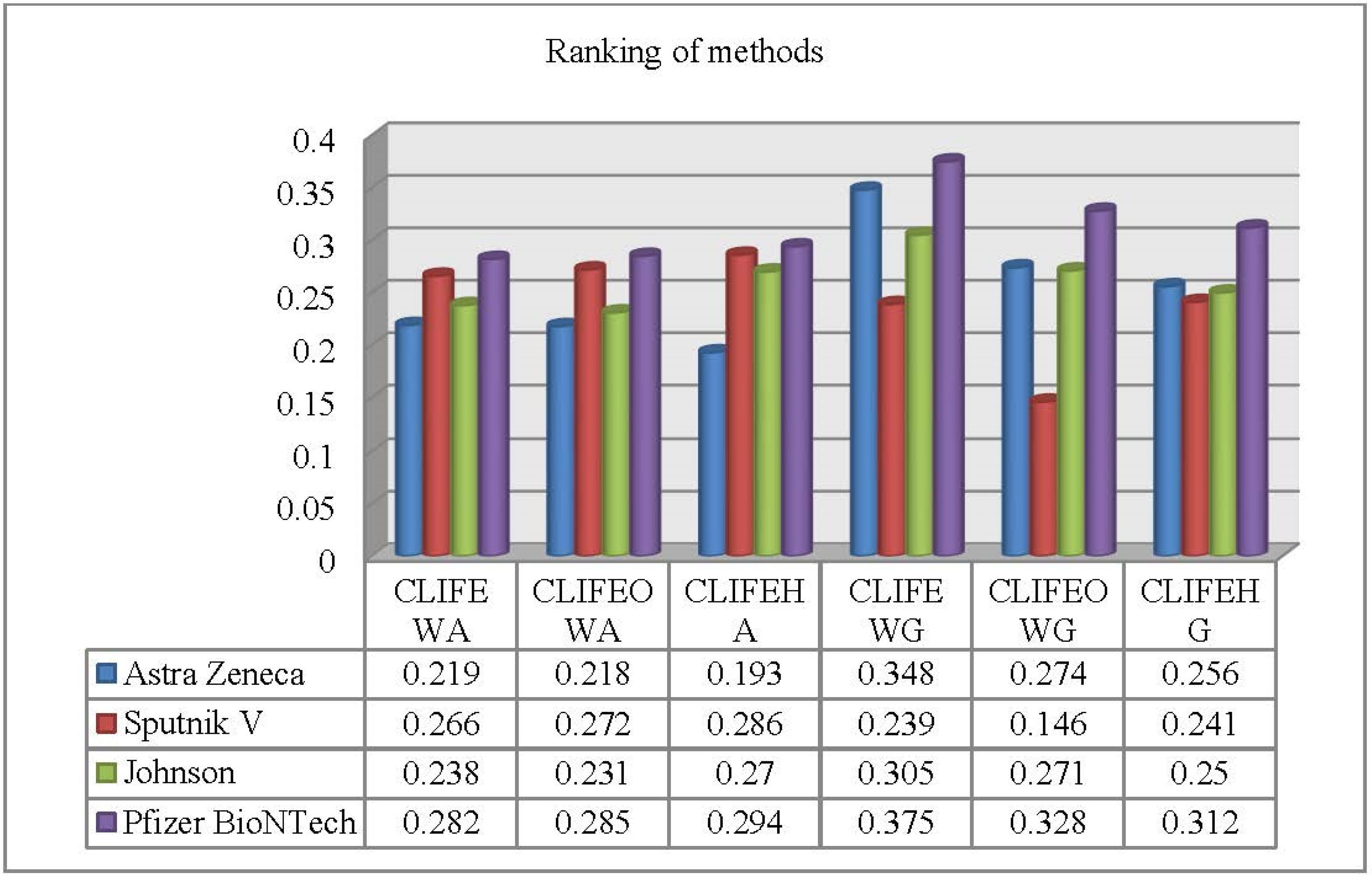
Case study: Several cases were found in Pakistan of the COVID-19 on March 2020. As, it was found first in China and declared by WHO a dangerous disease and may spread through communication and social interaction. Keeping in view the government of Pakistan wants to control the COVID-19 in Pakistan. For this, the government of Pakistan decided to specify some Vaccine. For this purpose Govt make a group of five experts doctors, such as $õ=\left\{{õ}_1,{õ}_2,{õ}_3,{õ}_4,{õ}_5\right\}$ for decision, whose weight is $\wp ={\left(0.1,0.2,0.2,0.2,0.3\right)}^T$. The doctors considered four best vaccine to control the COVID-19, such as ${\pounds }_1$: Astra Zeneca vaccine, ${\pounds }_2$: Sputnik V vaccine, ${\pounds }_3$: Johnson & Johnson’s Janssen vaccine, ${\pounds }_4$: Pfizer BioNTech Vaccine. Decision makers make a decision under some criteria of the proposed alternatives, such as ${\aleph }_1$: Drawbacks of the proposed vaccine, ${\aleph }_2$: Vaccine accessibility and availability, ${\aleph }_3$: Vaccine spending, ${\aleph }_4$: Qualities of the vaccine, whose weight is $þ={\left(0.1,0.2,0.3,0.4\right)}^T$. In the mentioned criteria, there are two form, such as ${\aleph }_1$, ${\aleph }_3$ are in the cost form and ${\aleph }_2$, ${\aleph }_4$ are in the benefit form. The given data have two types. Therefore, we have to normalize the given provided data.

Table 1. Decision matrix of ${õ}_1$.

	${\aleph }_1$	${\aleph }_2$	${\aleph }_3$	${\aleph }_4$
${\pounds }_1$	$\langle \left(0.30,0.40\right),0.70\rangle$	$\langle \left(0.50,0.40\right),0.30\rangle$	$\langle \left(0.30,0.60\right),0.80\rangle$	$\langle \left(0.50,0.30\right),0.60\rangle$
${\pounds }_2$	$\langle \left(0.40,0.50\right),0.20\rangle$	$\langle \left(0.50,0.30\right),0.60\rangle$	$\langle \left(0.40,0.50\right),0.60\rangle$	$\langle \left(0.40,0.50\right),0.60\rangle$
${\pounds }_3$	$\langle \left(0.30,0.60\right),0.20\rangle$	$\langle \left(0.60,0.30\right),0.80\rangle$	$\langle \left(0.50,0.40\right),0.50\rangle$	$\langle \left(0.60,0.30\right),0.50\rangle$
${\pounds }_4$	$\langle \left(0.50,0.40\right),0.30\rangle$	$\langle \left(0.60,0.30\right),0.20\rangle$	$\langle \left(0.40,0.60\right),0.04\rangle$	$\langle \left(0.50,0.40\right),0.40\rangle$

,

Table 2. Decision matrix of ${õ}_2$.

	${\aleph }_1$	${\aleph }_2$	${\aleph }_3$	${\aleph }_4$
${\pounds }_1$	$\langle \left(0.30,0.60\right),0.30\rangle$	$\langle \left(0.50,0.30\right),0.60\rangle$	$\langle \left(0.30,0.50\right),0.60\rangle$	$\langle \left(0.50,0.40\right),0.70\rangle$
${\pounds }_2$	$\langle \left(0.40,0.50\right),0.60\rangle$	$\langle \left(0.70,0.20\right),0.60\rangle$	$\langle \left(0.40,0.60\right),0.04\rangle$	$\langle \left(0.50,0.30\right),0.20\rangle$
${\pounds }_3$	$\langle \left(0.40,0.50\right),0.10\rangle$	$\langle \left(0.60,0.30\right),0.50\rangle$	$\langle \left(0.40,0.50\right),0.30\rangle$	$\langle \left(0.60,0.30\right),0.80\rangle$
${\pounds }_4$	$\langle \left(0.50,0.40\right),0.40\rangle$	$\langle \left(0.50,0.40\right),0.50\rangle$	$\langle \left(0.50,0.40\right),0.30\rangle$	$\langle \left(0.60,0.30\right),0.20\rangle$

,

Table 3. Decision matrix of ${õ}_3$.

	${\aleph }_1$	${\aleph }_2$	${\aleph }_3$	${\aleph }_4$
${\pounds }_1$	$\langle \left(0.30,0.70\right),0.60\rangle$	$\langle \left(0.50,0.20\right),0.70\rangle$	$\langle \left(0.40,0.50\right),0.30\rangle$	$\langle \left(0.50,0.40\right),0.60\rangle$
${\pounds }_2$	$\langle \left(0.40,0.60\right),0.04\rangle$	$\langle \left(0.70,0.20\right),0.60\rangle$	$\langle \left(0.40,0.40\right),0.30\rangle$	$\langle \left(0.50,0.30\right),0.20\rangle$
${\pounds }_3$	$\langle \left(0.40,0.50\right),0.30\rangle$	$\langle \left(0.60,0.30\right),0.80\rangle$	$\langle \left(0.40,0.50\right),0.10\rangle$	$\langle \left(0.60,0.30\right),0.50\rangle$
${\pounds }_4$	$\langle \left(0.50,0.40\right),0.30\rangle$	$\langle \left(0.60,0.30\right),0.20\rangle$	$\langle \left(0.50,0.40\right),0.40\rangle$	$\langle \left(0.50,0.40\right),0.50\rangle$

,

Table 4. Decision matrix of ${õ}_4$.

	${\aleph }_1$	${\aleph }_2$	${\aleph }_3$	${\aleph }_4$
${\pounds }_1$	$\langle \left(0.40,0.50\right),0.10\rangle$	$\langle \left(0.40,0.40\right),0.30\rangle$	$\langle \left(0.30,0.60\right),0.80\rangle$	$\langle \left(0.50,0.30\right),0.60\rangle$
${\pounds }_2$	$\langle \left(0.50,0.40\right),0.40\rangle$	$\langle \left(0.50,0.30\right),0.60\rangle$	$\langle \left(0.40,0.50\right),0.60\rangle$	$\langle \left(0.60,0.30\right),0.50\rangle$
${\pounds }_3$	$\langle \left(0.30,0.60\right),0.20\rangle$	$\langle \left(0.60,0.30\right),0.80\rangle$	$\langle \left(0.50,0.40\right),0.50\rangle$	$\langle \left(0.60,0.30\right),0.50\rangle$
${\pounds }_4$	$\langle \left(0.50,0.40\right),0.30\rangle$	$\langle \left(0.60,0.30\right),0.20\rangle$	$\langle \left(0.40,0.60\right),0.04\rangle$	$\langle \left(0.50,0.40\right),0.40\rangle$

and

Table 5. Decision matrix of ${õ}_5$.

	${\aleph }_1$	${\aleph }_2$	${\aleph }_3$	${\aleph }_4$
${\pounds }_1$	$\langle \left(0.40,0.50\right),0.10\rangle$	$\langle \left(0.50,0.40\right),0.50\rangle$	$\langle \left(0.40,0.60\right),0.04\rangle$	$\langle \left(0.60,0.30\right),0.20\rangle$
${\pounds }_2$	$\langle \left(0.40,0.50\right),0.60\rangle$	$\langle \left(0.70,0.20\right),0.60\rangle$	$\langle \left(0.30,0.50\right),0.60\rangle$	$\langle \left(0.50,0.30\right),0.20\rangle$
${\pounds }_3$	$\langle \left(0.30,0.60\right),0.30\rangle$	$\langle \left(0.60,0.30\right),0.50\rangle$	$\langle \left(0.40,0.50\right),0.30\rangle$	$\langle \left(0.60,0.30\right),0.80\rangle$
${\pounds }_4$	$\langle \left(0.50,0.40\right),0.40\rangle$	$\langle \left(0.50,0.30\right),0.60\rangle$	$\langle \left(0.50,0.40\right),0.30\rangle$	$\langle \left(0.50,0.40\right),0.70\rangle$

having information of the experts and

Table 6. Normalized matrix of ${õ}_1$.

	${\aleph }_1$	${\aleph }_2$	${\aleph }_3$	${\aleph }_4$
${\pounds }_1$	$\langle \left(0.40,0.30\right),0.70\rangle$	$\langle \left(0.50,0.40\right),0.30\rangle$	$\langle \left(0.60,0.30\right),0.80\rangle$	$\langle \left(0.50,0.30\right),0.60\rangle$
${\pounds }_2$	$\langle \left(0.50,0.40\right),0.20\rangle$	$\langle \left(0.50,0.30\right),0.60\rangle$	$\langle \left(0.50,0.40\right),0.60\rangle$	$\langle \left(0.40,0.50\right),0.60\rangle$
${\pounds }_3$	$\langle \left(0.60,0.30\right),0.20\rangle$	$\langle \left(0.60,0.30\right),0.80\rangle$	$\langle \left(0.40,0.50\right),0.50\rangle$	$\langle \left(0.60,0.30\right),0.50\rangle$
${\pounds }_4$	$\langle \left(0.40,0.50\right),0.30\rangle$	$\langle \left(0.60,0.30\right),0.20\rangle$	$\langle \left(0.60,0.40\right),0.04\rangle$	$\langle \left(0.50,0.40\right),0.40\rangle$

,

Table 7. Normalized matrix of ${õ}_2$.

	${\aleph }_1$	${\aleph }_2$	${\aleph }_3$	${\aleph }_4$
${\pounds }_1$	$\langle \left(0.60,0.30\right),0.30\rangle$	$\langle \left(0.50,0.30\right),0.60\rangle$	$\langle \left(0.50,0.30\right),0.60\rangle$	$\langle \left(0.50,0.40\right),0.70\rangle$
${\pounds }_2$	$\langle \left(0.50,0.40\right),0.60\rangle$	$\langle \left(0.70,0.20\right),0.60\rangle$	$\langle \left(0.60,0.40\right),0.40\rangle$	$\langle \left(0.50,0.30\right),0.20\rangle$
${\pounds }_3$	$\langle \left(0.50,0.40\right),0.10\rangle$	$\langle \left(0.60,0.30\right),0.50\rangle$	$\langle \left(0.50,0.40\right),0.30\rangle$	$\langle \left(0.60,0.30\right),0.80\rangle$
${\pounds }_4$	$\langle \left(0.40,0.50\right),0.40\rangle$	$\langle \left(0.50,0.40\right),0.50\rangle$	$\langle \left(0.40,0.50\right),0.30\rangle$	$\langle \left(0.60,0.30\right),0.20\rangle$

,

Table 8. Normalized matrix of ${õ}_3$.

	${\aleph }_1$	${\aleph }_2$	${\aleph }_3$	${\aleph }_4$
${\pounds }_1$	$\langle \left(0.70,0.30\right),0.60\rangle$	$\langle \left(0.50,0.20\right),0.70\rangle$	$\langle \left(0.50,0.40\right),0.30\rangle$	$\langle \left(0.50,0.40\right),0.60\rangle$
${\pounds }_2$	$\langle \left(0.60,0.40\right),0.40\rangle$	$\langle \left(0.70,0.20\right),0.60\rangle$	$\langle \left(0.40,0.40\right),0.30\rangle$	$\langle \left(0.50,0.30\right),0.20\rangle$
${\pounds }_3$	$\langle \left(0.50,0.40\right),0.30\rangle$	$\langle \left(0.60,0.30\right),0.80\rangle$	$\langle \left(0.50,0.40\right),0.10\rangle$	$\langle \left(0.60,0.30\right),0.50\rangle$
${\pounds }_4$	$\langle \left(0.40,0.50\right),0.30\rangle$	$\langle \left(0.60,0.30\right),0.20\rangle$	$\langle \left(0.40,0.50\right),0.40\rangle$	$\langle \left(0.50,0.40\right),0.50\rangle$

,

Table 9. Normalized matrix of ${õ}_4$.

	${\aleph }_1$	${\aleph }_2$	${\aleph }_3$	${\aleph }_4$
${\pounds }_1$	$\langle \left(0.50,0.40\right),0.10\rangle$	$\langle \left(0.40,0.40\right),0.30\rangle$	$\langle \left(0.60,0.30\right),0.80\rangle$	$\langle \left(0.50,0.30\right),0.60\rangle$
${\pounds }_2$	$\langle \left(0.40,0.50\right),0.40\rangle$	$\langle \left(0.50,0.30\right),0.60\rangle$	$\langle \left(0.50,0.40\right),0.60\rangle$	$\langle \left(0.60,0.30\right),0.50\rangle$
${\pounds }_3$	$\langle \left(0.60,0.30\right),0.20\rangle$	$\langle \left(0.60,0.30\right),0.80\rangle$	$\langle \left(0.40,0.50\right),0.50\rangle$	$\langle \left(0.60,0.30\right),0.50\rangle$
${\pounds }_4$	$\langle \left(0.40,0.50\right),0.30\rangle$	$\langle \left(0.60,0.30\right),0.20\rangle$	$\langle \left(0.60,0.40\right),0.40\rangle$	$\langle \left(0.50,0.40\right),0.40\rangle$

and

Table 10. Normalized matrix of ${õ}_5$.

	${\aleph }_1$	${\aleph }_2$	${\aleph }_3$	${\aleph }_4$
${\pounds }_1$	$\langle \left(0.50,0.40\right),0.10\rangle$	$\langle \left(0.50,0.40\right),0.50\rangle$	$\langle \left(0.60,0.40\right),0.40\rangle$	$\langle \left(0.60,0.30\right),0.20\rangle$
${\pounds }_2$	$\langle \left(0.50,0.40\right),0.60\rangle$	$\langle \left(0.70,0.20\right),0.60\rangle$	$\langle \left(0.50,0.30\right),0.60\rangle$	$\langle \left(0.50,0.30\right),0.20\rangle$
${\pounds }_3$	$\langle \left(0.60,0.30\right),0.30\rangle$	$\langle \left(0.60,0.30\right),0.50\rangle$	$\langle \left(0.50,0.40\right),0.30\rangle$	$\langle \left(0.60,0.30\right),0.80\rangle$
${\pounds }_4$	$\langle \left(0.40,0.50\right),0.40\rangle$	$\langle \left(0.50,0.30\right),0.60\rangle$	$\langle \left(0.40,0.50\right),0.30\rangle$	$\langle \left(0.50,0.40\right),0.70\rangle$

having information of the experts in normalized form.

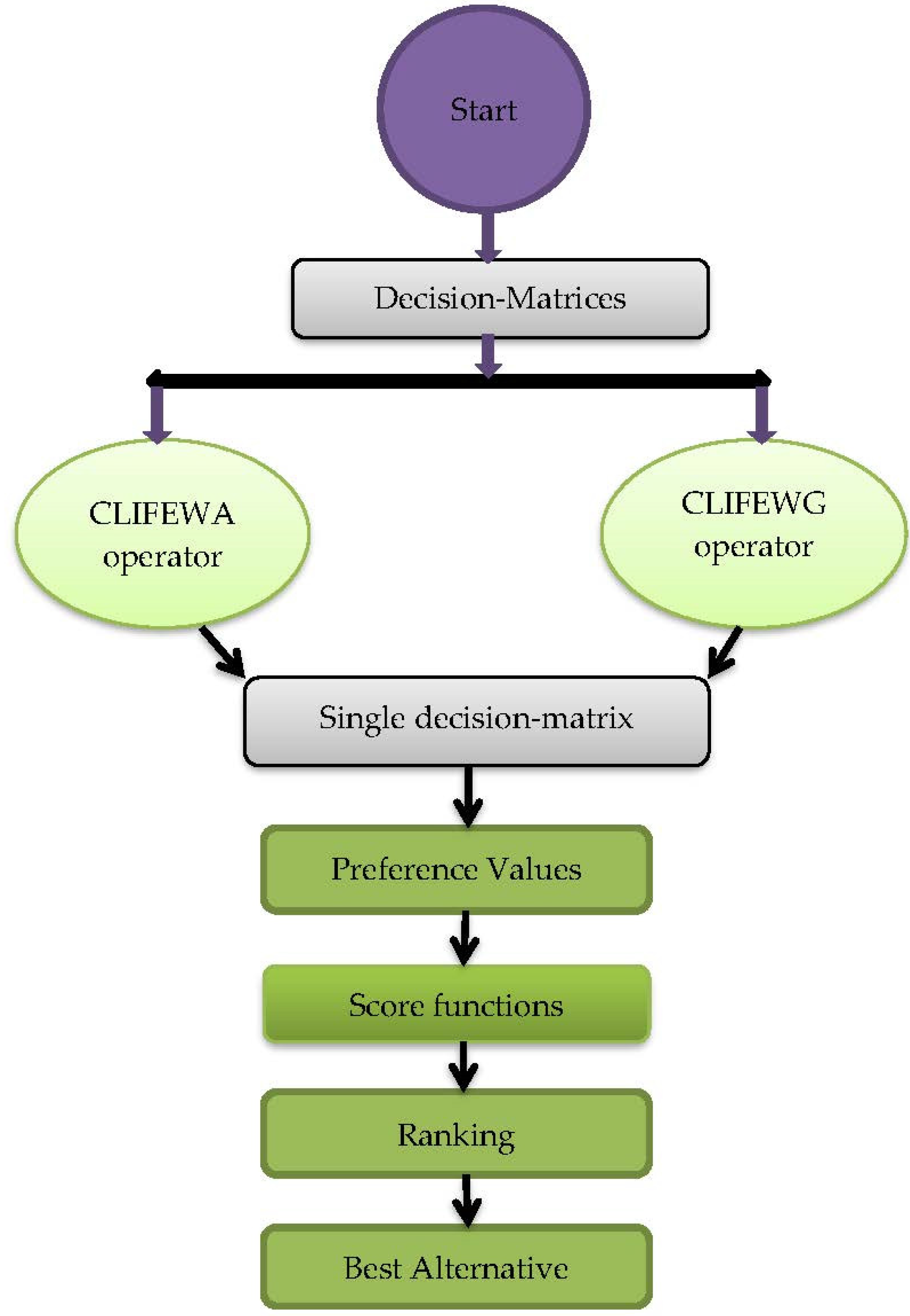
In the following Figure 1, we show the step by step process.

Step 1: Contract decision matrices based on the expert’s suggestions:

Step 2: Covert all decision-matrices into normalized matrices, and get Table 6, Table 7, Table 8, Table 9 and Table 10.

Step 3: By using CLIFEWA operator and CLIFEWG operator, with $\wp ={\left(0.10,0.20,0.20,0.20,0.30\right)}^T$ and $\alpha =0.2$.

Table 11. Collective normalized matrix under CLIFEWA operator.

	${\aleph }_1$	${\aleph }_2$	${\aleph }_3$	${\aleph }_4$
${\pounds }_1$	$\left(0.630,0.256\right)$	$\left(0.547,0.316\right)$	$\left(0.663,0.304\right)$	$\left(0.521,0.357\right)$
${\pounds }_2$	$\left(0.624,0.314\right)$	$\left(0.482,0.296\right)$	$\left(0.558,0.229\right)$	$\left(0.546,0.410\right)$
${\pounds }_3$	$\left(0.665,0.321\right)$	$\left(0.591,0.357\right)$	$\left(0.628,0.246\right)$	$\left(0.547,0.316\right)$
${\pounds }_4$	$\left(0.568,0.234\right)$	$\left(0.536,0.460\right)$	$\left(0.619,0.324\right)$	$\left(0.596,0.382\right)$

and

Table 12. Collective normalized matrix under CLIFEWG operator.

	${\aleph }_1$	${\aleph }_2$	${\aleph }_3$	${\aleph }_4$
${\pounds }_1$	$\left(0.624,0.216\right)$	$\left(0.544,0.312\right)$	$\left(0.667,0.324\right)$	$\left(0.527,0.351\right)$
${\pounds }_2$	$\left(0.614,0.310\right)$	$\left(0.478,0.291\right)$	$\left(0.558,0.229\right)$	$\left(0.546,0.410\right)$
${\pounds }_3$	$\left(0.665,0.321\right)$	$\left(0.593,0.357\right)$	$\left(0.628,0.246\right)$	$\left(0.547,0.316\right)$
${\pounds }_4$	$\left(0.563,0.224\right)$	$\left(0.532,0.458\right)$	$\left(0.623,0.322\right)$	$\left(0.601,0.362\right)$

having collective normalized matrix under CLIFEWA operator and collective normalized matrix under CLIFEWG operator respectively.

Step 4: Next, we make hybrid matrices, using Table 11, Table 12. First, we have to computing the hybrid values, such that ${\stackrel{.}{\mu }}_j=n{û}_j{\mu }_j$, ${\stackrel{.}{\mu }}_j={\left({\mu }_j\right)}^{n{û}_j}$, where $û={\left(0.10,0.20,0.30,0.40\right)}^T$ and get,

Table 13. Hybrid averaging matrix.

	${\aleph }_1$	${\aleph }_2$	${\aleph }_3$	${\aleph }_4$
${\pounds }_1$	$\left(0.571,0.226\right)$	$\left(0.588,0.295\right)$	$\left(0.728,0.239\right)$	$\left(0.660,0.192\right)$
${\pounds }_2$	$\left(0.627,0.320\right)$	$\left(0.660,0.319\right)$	$\left(0.624,0.170\right)$	$\left(0.611,0.288\right)$
${\pounds }_3$	$\left(0.622,0.352\right)$	$\left(0.475,0.238\right)$	$\left(0.694,0.185\right)$	$\left(0.494,0.245\right)$
${\pounds }_4$	$\left(0.578,0.254\right)$	$\left(0.676,0.337\right)$	$\left(0.685,0.258\right)$	$\left(0.536,0.336\right)$

,

Table 14. Hybrid geometric matrix.

	${\aleph }_1$	${\aleph }_2$	${\aleph }_3$	${\aleph }_4$
${\pounds }_1$	$\left(0.714,0.258\right)$	$\left(0.524,0.389\right)$	$\left(0.562,0.374\right)$	$\left(0.765,0.214\right)$
${\pounds }_2$	$\left(0.830,0.106\right)$	$\left(0.528,0.348\right)$	$\left(0.610,0.352\right)$	$\left(0.520,0.306\right)$
${\pounds }_3$	$\left(0.825,0.144\right)$	$\left(0.479,0.315\right)$	$\left(0.464,0.268\right)$	$\left(0.574,0.226\right)$
${\pounds }_4$	$\left(0.848,0.134\right)$	$\left(0.566,0.297\right)$	$\left(0.572,0.287\right)$	$\left(0.577,0.202\right)$

respectively. Table 13 and Table 14 having hybrid averaging and hybrid geometric data respectively.

Step 5: Using Table 11, Table 12, Table 13 and Table 14, where $þ={\left(0.1,0.2,0.3,0.4\right)}^T$, and get

Table 15. Preference values of all operators.

	${\pounds }_1$	${\pounds }_2$	${\pounds }_3$	${\pounds }_4$
CLIFEWA	$\left(0.537,0.328\right)$	$\left(0.588,0.325\right)$	$\left(0.523,0.295\right)$	$\left(0.494,0.214\right)$
CLIFEOWA	$\left(0.494,0.286\right)$	$\left(0.491,0.229\right)$	$\left(0.498,0.287\right)$	$\left(0.488,0.239\right)$
CLIFEHA	$\left(0.449,0.220\right)$	$\left(0.489,0.297\right)$	$\left(0.496,0.221\right)$	$\left(0.510,0.218\right)$
CLIFEWG	$\left(0.604,0.257\right)$	$\left(0.549,0.311\right)$	$\left(0.559,0.255\right)$	$\left(0.598,0.224\right)$
CLIFEOWG	$\left(0.546,0.273\right)$	$\left(0.525,0.381\right)$	$\left(0.546,0.273\right)$	$\left(0.525,0.381\right)$
CLIFEHG	$\left(0.489,0.243\right)$	$\left(0.497,0.258\right)$	$\left(0.581,0.345\right)$	$\left(0.522,0.221\right)$

and

Table 16. Scores of all methods.

Operators	Score Functions	Ranking
CLIFEWA	$0.219, 0.266, 0.238, 0.282$	${\pounds }_4\succ {\pounds }_2\succ {\pounds }_3\succ {\pounds }_1$
CLIFEOWA	$0.218, 0.272, 0.231, 0.285$	${\pounds }_4\succ {\pounds }_2\succ {\pounds }_3\succ {\pounds }_1$
CLIFEHA	$0.193, 0.286, 0.270, 0.294$	${\pounds }_4\succ {\pounds }_2\succ {\pounds }_3\succ {\pounds }_1$
CLIFEWG	$0.348, 0.239, 0.305, 0.375$	${\pounds }_4\succ {\pounds }_1\succ {\pounds }_3\succ {\pounds }_2$
CLIFEOWG	$0.274, 0.146, 0.271, 0.328$	${\pounds }_4\succ {\pounds }_1\succ {\pounds }_3\succ {\pounds }_2$
CLIFEHG	$0.256, 0.241, 0.250, 0.312$	${\pounds }_4\succ {\pounds }_1\succ {\pounds }_3\succ {\pounds }_2$

respectively. Table 15, contains all preference values and Table 16 contains their score functions respectively.

5. Comparative and Sensitive Analysis

Intuitionistic fuzzy set is one of the successful generalizations of their existing study such as fuzzy sets, by considering much more information related to an object during the process. For example, fuzzy sets contains only membership grade, but intuitionistic fuzzy sets contain both membership grade and non-membership grade under attentions, such that their sum is less than or equal to one. In

Table 17. Comparisons with existing operators.

Averaging Approaches	Ordering	Geometric Approaches	Ordering
IFWA [9]	${\pounds }_4\succ {\pounds }_1\succ {\pounds }_2\succ {\pounds }_3$	IFWG [8]	${\pounds }_4\succ {\pounds }_1\succ {\pounds }_2\succ {\pounds }_3$
IFOWA [9]	${\pounds }_4\succ {\pounds }_1\succ {\pounds }_2\succ {\pounds }_3$	IFOWG [8]	${\pounds }_4\succ {\pounds }_1\succ {\pounds }_2\succ {\pounds }_3$
IFHA [9]	${\pounds }_4\succ {\pounds }_1\succ {\pounds }_3\succ {\pounds }_2$	IFHG [8]	${\pounds }_4\succ {\pounds }_1\succ {\pounds }_3\succ {\pounds }_2$
IFEWA [13]	${\pounds }_4\succ {\pounds }_2\succ {\pounds }_1\succ {\pounds }_3$	IFEWG [12]	${\pounds }_4\succ {\pounds }_1\succ {\pounds }_2\succ {\pounds }_3$
IFEOWA [13]	${\pounds }_4\succ {\pounds }_2\succ {\pounds }_1\succ {\pounds }_3$	IFEOWG [12]	${\pounds }_4\succ {\pounds }_1\succ {\pounds }_2\succ {\pounds }_3$
IFEHA [14]	${\pounds }_4\succ {\pounds }_2\succ {\pounds }_1\succ {\pounds }_3$	IFEHG [14]	${\pounds }_4\succ {\pounds }_1\succ {\pounds }_2\succ {\pounds }_3$
LIFWA [41]	${\pounds }_4\succ {\pounds }_1\succ {\pounds }_3\succ {\pounds }_2$	LIFWG [41]	${\pounds }_4\succ {\pounds }_1\succ {\pounds }_3\succ {\pounds }_2$
LIFOWA [41]	${\pounds }_4\succ {\pounds }_1\succ {\pounds }_3\succ {\pounds }_2$	LIFOWG [41]	${\pounds }_4\succ {\pounds }_1\succ {\pounds }_3\succ {\pounds }_2$
CIFWA [44]	$A_4\succ A_1\succ A_2\succ A_3$	CIFWG [44]	${\pounds }_4\succ {\pounds }_1\succ {\pounds }_2\succ {\pounds }_3$
CIFOWA [44]	${\pounds }_4\succ {\pounds }_1\succ {\pounds }_2\succ {\pounds }_3$	CIFOWG [44]	${\pounds }_4\succ {\pounds }_1\succ {\pounds }_2\succ {\pounds }_3$
CIFEWA [44]	${\pounds }_4\succ {\pounds }_2\succ {\pounds }_1\succ {\pounds }_3$	CIFEWG [44]	${\pounds }_4\succ {\pounds }_2\succ {\pounds }_1\succ {\pounds }_3$
CIFEOWA [44]	${\pounds }_4\succ {\pounds }_2\succ {\pounds }_1\succ {\pounds }_3$	CIFEOWG [44]	${\pounds }_4\succ {\pounds }_2\succ {\pounds }_1\succ {\pounds }_3$
CIFHA [43]	${\pounds }_4\succ {\pounds }_2\succ {\pounds }_1\succ {\pounds }_3$	CIFHG [43]	${\pounds }_4\succ {\pounds }_1\succ {\pounds }_3\succ {\pounds }_2$
CLIFEWA	${\pounds }_4\succ {\pounds }_2\succ {\pounds }_3\succ {\pounds }_1$	CLIFEWG	${\pounds }_4\succ {\pounds }_2\succ {\pounds }_3\succ {\pounds }_1$
CLIFEOWA	${\pounds }_4\succ {\pounds }_2\succ {\pounds }_3\succ {\pounds }_1$	CLIFEOWG	${\pounds }_4\succ {\pounds }_2\succ {\pounds }_3\succ {\pounds }_1$
CLIFEHA	${\pounds }_4\succ {\pounds }_2\succ {\pounds }_3\succ {\pounds }_1$	CLIFEHG	${\pounds }_4\succ {\pounds }_2\succ {\pounds }_3\succ {\pounds }_1$

, we present the comparative analysis of the novel approaches to their existing approaches.

In the following Figure 2, we show the graphical representation of all proposed methods.

6. Conclusions

In this paper, we have developed Einstein sum and Einstein product which are the good alternatives of algebraic sum and product. We have developed several new LOLs for intuitionistic fuzzy sets with real base number $\alpha$, under confidence level. Additionally, we have presented several Einstein operators under confidence environment, such as the CLIFEWA operator, the CLIFEOWA operator, the CLIFEHA operator, the CLIFEWG operator, the CLIFEOWG operator, and the CLIFEHG operator. A comparative study was performed with some recent studies to demonstrate their superiority and the legitimacy. Finally, the proposed approaches are utilized on MAGDM problem to demonstrate the legality, applicability and effectiveness of these new methods. But, the proposed methods have some limitations, such that for all real numbers, such that ${\log }_1\left(\mu \right)$ and ${\log }_{\alpha }\left(0\right)$ are not defined. Similarly if $\alpha$ be a real number and $\mu$ be an intuitionistic fuzzy value, then ${\log }_{\alpha }\left(\mu \right)$ cannot be calculated for $\mu =0$ and $\alpha =1$. Hence throughout in this research, we consider that $\mu \ne 0$ and $\alpha \ne 1$.

Furthermore, this study can be expanded to complex Dombi approaches under confidence level, complex Logarithmic approach under confidence level, complex geometric approach under confidence level, complex linguistic terms, complex symmetric operators under confidence level, complex power operators under confidence level, complex Hamacher operators under confidence level, complex Einstein approaches under confidence level, complex confidence level, complex interval-valued approaches, complex Hamacher interval approaches, complex Einstein interval approaches, complex Dombi interval approaches under confidence level, etc.

References

- Molodtsov, D. Soft set theory—First results. Comput. Math. Appl. 1999, 37, 19–31. [Google Scholar] [CrossRef]
- Pawlak, Z. Rough sets. Int. J. Comput. Inform. Sci. 1982, 11, 341–356. [Google Scholar] [CrossRef]
- Zadeh, L.A. Fuzzy sets. Inf. Control 1965, 8, 338–353. [Google Scholar] [CrossRef]
- Atanassov, K.T. Intuitionistic fuzzy sets. Fuzzy Sets Syst. 1986, 20, 87–96. [Google Scholar] [CrossRef]
- Atanassov, K.T.; Gargov, G. Interval valued intuitionistic fuzzy sets. Fuzzy Sets Syst. 1989, 31, 343–349. [Google Scholar] [CrossRef]
- Yager, R.R.; Kacprzyk, J. The Ordered Weighted Averaging Operators: Theory and Applications; Kluwer Academic Publisher: Boston, MA, USA, 1997. [Google Scholar]
- Yager, R.R. On ordered weighted averaging aggregation operators in multi criteria decision making. IEEE Trans. Syst. Man Cybern. 1988, 18, 183–190. [Google Scholar] [CrossRef]
- Xu, Z.S.; Yager, R.R. Some geometric aggregation operators based on intuitionistic fuzzy sets. Int. J. Gen. Syst. 2006, 35, 417–433. [Google Scholar] [CrossRef]
- Xu, Z.S. Intuitionistic fuzzy aggregation operators. IEEE Trans Fuzzy Syst. 2007, 15, 1179–1187. [Google Scholar]
- Ye, J. Improved method of multi criteria fuzzy decision making based on vague sets. Comput. Aided Des. 2007, 39, 164–169. [Google Scholar] [CrossRef]
- Ye, J. Multicriteria fuzzy decision-making method based on a novel accuracy function under interval-valued intuitionistic fuzzy environment. Expert Syst. Appl. 2009, 36, 6899–6902. [Google Scholar] [CrossRef]
- Wang, W.; Liu, X. Intuitionistic Fuzzy Geometric Aggregation Operators Based on Einstein Operations. Int. J. Intell. Syst. 2011, 26, 1049–1075. [Google Scholar] [CrossRef]
- Wang, W.; Liu, X. Intuitionistic fuzzy information aggregation using Einstein operations. IEEE Trans. Fuzzy Syst. 2012, 20, 923–938. [Google Scholar] [CrossRef]
- Zhao, X.; Wei, G. Some intuitionistic fuzzy Einstein hybrid aggregation operators and their application to multiple attribute decision making. Knowl. Based Syst. 2013, 37, 472–479. [Google Scholar] [CrossRef]
- Xu, Y.; Wang, H.; Merigo, J.M. Intuitionistic fuzzy Einstein choquet integral operators for multiple attribute decision making. Technol. Econ. Dev. Econ. 2014, 20, 227–253. [Google Scholar] [CrossRef]
- Garg, H. Generalized intuitionistic fuzzy interactive geometric interaction operators using Einstein t-norm and t-conorm and their application to decision making. Comput. Ind. Eng. 2016, 101, 53–69. [Google Scholar] [CrossRef]
- Garg, H. Generalized intuitionistic fuzzy multiplicative interactive geometric operators and their application to multiple criteria decision making. Int. J. Mach. Learn. Cybern. 2016, 7, 1075–1092. [Google Scholar] [CrossRef]
- Garg, H. A new generalized improved score function of interval-valued intuitionistic fuzzy sets and applications in expert systems. Appl. Soft Comput. 2016, 38, 988–999. [Google Scholar] [CrossRef]
- Nancy, G.H.; Garg, H. Novel single-valued neutrosophic decision making operators under frank norm operations and its application. Int. J. Uncertain. Quantif. 2016, 6, 361–375. [Google Scholar] [CrossRef]
- Garg, H. An improved score function for ranking neutrosophic sets and its application to decision-making process. Int. J. Uncertain. Quantif. 2016, 6, 377–385. [Google Scholar]
- Sarfraz, M.; Ullah, K.; Akram, M.; Pamucar, D.; Božanić, D. Prioritized Aggregation Operators for Intuitionistic Fuzzy Information Based on Aczel–Alsina T-Norm and T-Conorm and Their Applications in Group Decision-Making. Symmetry 2022, 14, 2655. [Google Scholar] [CrossRef]
- Yu, D.; Shi, S. Researching the development of Atanassov intuitionistic fuzzy set: Using a citation network analysis. Appl. Soft Comput. 2015, 32, 189–198. [Google Scholar] [CrossRef]
- Garg, H.; Agarwal, N.; Tripathi, A. Entropy based multi-criteria decision making method under fuzzy environment and unknown attribute weights. Glob. J. Technol. Optim. 2015, 6, 13–20. [Google Scholar]
- Dalman, H.; Guzel, N.; Sivri, M. A fuzzy set-based approach to multi objective multi-item solid transportation problem under uncertainty. Int. J. Fuzzy Syst. 2016, 18, 716–729. [Google Scholar] [CrossRef]
- Kumar, K.; Garg, H. TOPSIS method based on the connection number of set pair analysis under interval-valued intuitionistic fuzzy set environment. Comput. Appl. Math. 2016, 37, 1319–1329. [Google Scholar] [CrossRef]
- Gou, X.J.; Xu, Z.S.; Lei, Q. New operational laws and aggregation method of intuitionistic fuzzy information. J. Intell. Fuzzy Syst. 2016, 30, 129–141. [Google Scholar] [CrossRef]
- Rahman, K.; Abdullah, S.; Jamil, M.; Khan, M.Y. Some generalized intuitionistic fuzzy Einstein hybrid aggregation operators and their application to multiple- attribute group decision-making. Int. J. Fuzzy Syst. 2018, 20, 1567–1575. [Google Scholar] [CrossRef]
- Jamil, M.; Rahman, K.; Abdullah, S.; Khan, M.Y. The Induced Generalized Interval-Valued Intuitionistic Fuzzy Einstein Hybrid Geometric Aggregation Operator and Their Application to Group Decision-Making. J. Intell. Fuzzy Syst. 2020, 38, 1737–1752. [Google Scholar] [CrossRef]
- Huynh, N.T.; Nguyen, V.T.; Nguyen, Q.M. Optimum Design for the Magnification Mechanisms Employing Fuzzy Logic–ANFIS. Comput. Mater. Contin. 2022, 73, 5961–5983. [Google Scholar] [CrossRef]
- Peng, F.; Wang, Y.; Xuan, H.; Nguyen, T.V.T. Efficient road traffic anti-collision warning system based on fuzzy nonlinear programming. Int. J. Syst. Assur. Eng. Manag. 2022, 13, S456–S461. [Google Scholar] [CrossRef]
- Nguyen, T.V.T.; Huynh, N.T.; Vu, N.C.; Kieu, V.N.D.; Huang, S.C. Optimizing compliant gripper mechanism design by employing an effective bi-algorithm: Fuzzy logic and ANFIS. Microsyst. Technol. 2021, 27, 3389–3412. [Google Scholar] [CrossRef]
- Atanassov, K.; Sotirova, E.; Andonov, V. Generalized Net Model of Multicriteria Decision Making Procedure Using Intercriteria Analysis. In Advances in Fuzzy Logic and Technology 2017; Advances in Intelligent Systems and Computing Book Series; Springer International Publishing: Cham, Switzerland, 2018. [Google Scholar] [CrossRef]
- Gergin, R.E.; Peker, İ.; Gök Kısa, A.C. Supplier selection by integrated IFDEMATEL-IFTOPSIS Method: A case study of automotive supply industry. Decis. Mak. Appl. Manag. Eng. 2022, 5, 169–193. [Google Scholar] [CrossRef]
- Khan, V.A.; Tuba, U.; Ashadul Rahaman, S.K. Motivations and Basics of Fuzzy, Intuitionistic Fuzzy and Neutrosophic Sets and Norms. Yugosl. J. Oper. Res. 2022, 32, 299–323. [Google Scholar] [CrossRef]
- Milovanović, V.R.; Aleksić, A.V.; Sokolović, V.S.; Milenkov, M.A. Uncertainty modeling using intuitionistic fuzzy numbers. Mil. Tech. Cour. 2021, 69, 905–929. [Google Scholar]
- Jovčić, S.; Průša, P.; Dobrodolac, M.; Švadlenka, L. A Proposal for a Decision-Making Tool in Third-Party Logistics (3PL) Provider Selection Based on Multi-Criteria Analysis and the Fuzzy Approach. Sustainability 2019, 11, 4236. [Google Scholar] [CrossRef]
- Zhou, B.; Chen, J.; Wu, Q.; Pamučar, D.; Wang, W.; Zhou, L. Risk priority evaluation of power transformer parts based on hybrid FMEA framework under hesitant fuzzy environment. Facta Univ. Ser. Mech. Eng. 2022, 20, 399–420. [Google Scholar] [CrossRef]
- Ashraf, A.; Ullah, K.; Hussain, A.; Bari, M. Interval-Valued Picture Fuzzy Maclaurin Symmetric Mean Operator with application in Multiple Attribute Decision-Making. Rep. Mech. Eng. 2022, 3, 210–226. [Google Scholar] [CrossRef]
- Yang, X.; Mahmood, T.; ur Rehman, U. Bipolar Complex Fuzzy Subgroups. Mathematics 2022, 10, 2882. [Google Scholar] [CrossRef]
- Li, Z.; Wei, F. The logarithmic operational laws of intuitionistic fuzzy sets and intuitionistic fuzzy numbers. J. Intell. Fuzzy Syst. 2017, 33, 3241–3253. [Google Scholar] [CrossRef]
- Rahman, K. Some new logarithmic aggregation operators and their application to group decision making problem based on t-norm and t-conorm. Soft Comput. 2022, 6, 2751–2772. [Google Scholar] [CrossRef]
- Ma, Z.; Zeng, S. Confidence Intuitionistic Fuzzy Hybrid Weighted Operator and its Application in Multi-Criteria Decision Making. J. Discret. Math. Sci. Cryptogr. 2014, 17, 529–538. [Google Scholar] [CrossRef]
- Yu, D. Intuitionistic fuzzy information aggregation under confidence levels. Appl. Soft Comput. 2014, 19, 147–160. [Google Scholar] [CrossRef]
- Yu, D. A scientometrics review on aggregation operator research. Scientometrics 2015, 105, 115–133. [Google Scholar] [CrossRef]
- Rahman, K. Decision-making problem based on confidence intuitionistic Trapezoidal fuzzy Einstein aggregation operators and their application. New Math. Nat. Comput. 2022, 18, 219–250. [Google Scholar] [CrossRef]
Figure 1.
Flowchart of the proposed approach.
Figure 2.
Graphical representation of the ranking of all methods.