

Reactor Temperature Control Based on Improved Fractional Order Self-Anti-Disturbance

Abstract
:1. Introduction
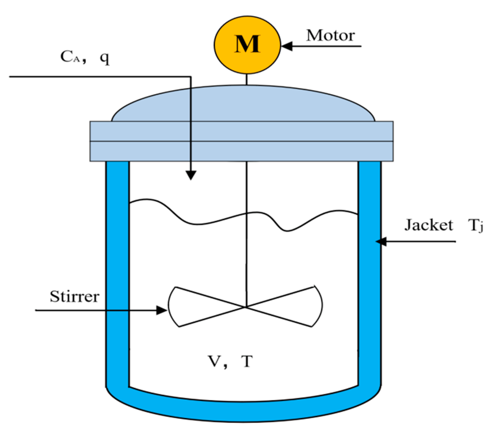
2. Reactor System Modeling
Reaction Tank Modeling
3. Control Strategy of Reaction Tank
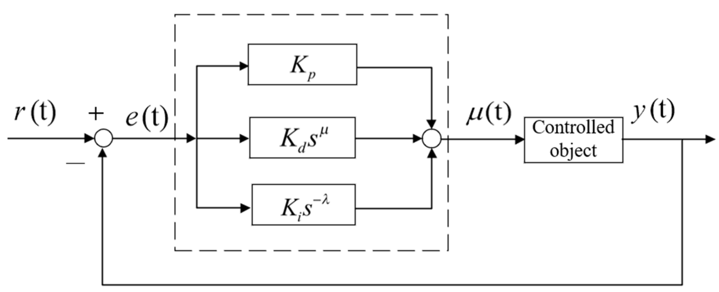
3.1. Fractional Order Controller
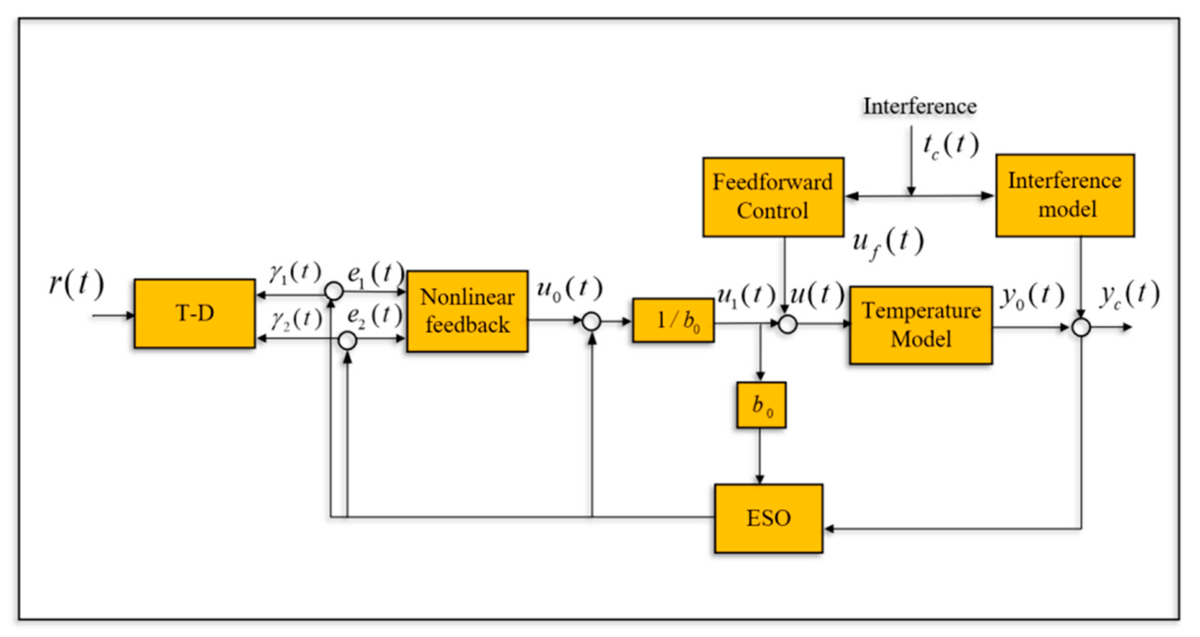
3.2. Feedforward Self-Anti-Disturbance Controller Design
3.3. Fractional Order Feedforward Self-Anti-Disturbance Controller Design
3.3.1. Improving Nonlinear Functions
3.3.2. FOTD
3.3.3. FOESO
3.3.4. FOPID
4. Simulation Experiments
5. Conclusions
Author Contributions
Funding
Informed Consent Statement
Data Availability Statement
Conflicts of Interest
References
- Vojtesek, J.; Dostal, P. Control of concentration inside CSTR using nonlinear adaptive controller. In Nostradamus 2014: Prediction, Modeling and Analysis of Complex Systems; Zelinka, I., Suganthan, P.N., Chen, G., Snasel, V., Abraham, A., Rössler, O., Eds.; Springer International Publishing: Berlin/Heidelberg, Germany, 2014; pp. 195–204. [Google Scholar]
- Zhu, B. Introduction to Active Disturbance Rejection Control; Beijing University of Aeronautics and Astronautics Press: Beijing, China, 2017. [Google Scholar]
- Guan, Z. Research on the Control Performance of Active Disturbance Rejection Controller for a Class of Thermal Objects. J. Therm. Energy Power Eng. 2011, 26, 495–496. [Google Scholar]
- Wu, Z.; He, T.; Li, D. Superheated steam temperature control based on modified active disturbance rejection control. Control. Eng. Pract. 2019, 83, 83–97. [Google Scholar] [CrossRef]
- Chen, Z.; Hao, Y.; Sun, L.; Su, Z. Phase compensation based active disturbance rejection control for high order superheated steam temperature system. Control. Eng. Pract. 2022, 126, 105200. [Google Scholar] [CrossRef]
- Jin, X.; Tong, B.; Ruan, X.; Wang, J. Process model and Active disturbance rejection temperature control of PTFE semi-batch polymerizatio. J. Cent. South Univ. 2020, 51, 1534–1541. [Google Scholar]
- Chen, Y.; Luo, Y.; Zheng, W.; Gao, Z.; Chen, Y. Fractional order active disturbance rejection control with the idea of cascaded fractional order integrator equivalence. ISA Trans. 2021, 114, 359–369. [Google Scholar] [CrossRef]
- Li, D.; Ding, P.; Gao, Z. Fractional active disturbance rejection control. ISA Trans. 2016, 61, 109–119. [Google Scholar] [CrossRef]
- Yi, H.; Wang, P.; Zhao, G. Fractional order active disturbance rejection control design for non-integer order plus time delay models. Trans. Inst. Meas. Control 2022, 01423312221140631. [Google Scholar] [CrossRef]
- Zhang, Z.; Cheng, J.; Guo, Y. PD-Based Optimal ADRC with Improved Linear Extended State Observer. Entropy 2021, 23, 888. [Google Scholar] [CrossRef]
- Wu, Z.; Li, D.; Chen, Y. Performance Analysis of Improved ADRCs for a Class of High-Order Processes With Verification on Main Steam Pressure Control. IEEE Trans. Ind. Electron. 2023, 70, 6180–6190. [Google Scholar] [CrossRef]
- Nosheen, T.; Ali, A.; Chaudhry, M.U.; Nazarenko, D.; Shaikh, I.u.H.; Bolshev, V.; Iqbal, M.M.; Khalid, S.; Panchenko, V. A Fractional Order Controller for Sensorless Speed Control of an Induction Motor. Energies 2023, 16, 1901. [Google Scholar] [CrossRef]
- Sun, S.; Hu, D.; Yu, Y.; Sun, J. Simulation and amplification design of flow heat transfer in reactor. Chem. Equip. Technol. 2018, 39, 20–23. [Google Scholar]
- Zhang, J. Research on Motion Control of Anchoring Robot Arm Based on WOA-FOPID Algorithm. Coal Sci. Technol. 2022, 50, 292–302. [Google Scholar]
- Yin, C.; Chen, Y.; Zhong, S. Fractional-order sliding modebased extremum seeking control of a class of nonlinear systems. Automatica 2014, 50, 3173–3181. [Google Scholar] [CrossRef]
- Al-Saggaf, U.M.; Mansouri, R.; Bettayeb, M.; Mehedi, I.M.; Munawar, K. Robustness Improvement of the Fractional order LADRC scheme for Integer High order system. IEEE Trans. Ind. Electron. 2021, 68, 8572–8581. [Google Scholar] [CrossRef]
- Sheng, Y.; Xie, Y.; Bai, W. Fractional-order sliding mode control for hypersonic vehicles with neural network disturbance compensator. Nonlinear Dyn. 2021, 103, 849–863. [Google Scholar] [CrossRef]
- Moltumyra, H.; Ragazzon, M.; Cravdahl, J. Fractional-orderco-ntrol;nyquist constrained optimization. IFAC PapersOnLine 2020, 53, 8605–8612. [Google Scholar] [CrossRef]
- Petero, J.; Shaikh, A.; Ibrahim, M.; Nisar, K.S.; Baleanu, D.; Khan, I.; Abioye, A.I. Analysis and dyna-mics of fractional order mathematical model of covid-19 in nigeria u-sing atangana-baleanu operator. Comput. Mater. Contin. 2021, 66, 1823–1848. [Google Scholar]
- Musarratm, N.; Fekih, A. A fractional order sliding mode cont-rol-based topology to improve the transient stability of wind energysystems. Int. J. Electr. Power Energy Syst. 2021, 133, 107306. [Google Scholar] [CrossRef]
- Podlubny, I. Fractional order systems and fractionalord controller. Math. Sci. Eng. 1999, 198, 243–260. [Google Scholar]
- Wu, X.; Liu, S.; Wang, Y. Stability analysis of Riemann-Liouvillefractional-order neural networks with reaction—Diffusion terms andmixed time—Varying delays. Neurocomputing 2021, 431, 169–178. [Google Scholar] [CrossRef]
- Labbadi, M.; Boukal, Y.; Cherkaoui, M. High order fractionalcontroller based on PID-SMC for the OUAV under uncertainties anddisturbance. In Advanced Robust Nonlinear Control Approaches for Ouadrotor Unmanned Aerial Vehicle; Springer: Cham, Switzerland, 2022. [Google Scholar]
- Da, W.; Ding, F.; Liu, N. Stabilization of uncertain fraction-al memristor chaotic time-delay system based on fractional order sliding mode control. J. Harbin Inst. Technol. 2020, 27, 78–87. [Google Scholar]
- Alhelou, M.; Gavrilov, A. Synthesis of active disturbance rejection control. Her. Bauman Mosc. State Tech. Univ. Ser. Instrum. Eng. 2020, 4, 22–41. [Google Scholar] [CrossRef]
- Jin, H.; Song, J.; Lan, W. On the characteristics of ADRC: A PID interpretation. Sci. China Inf. Sci. 2020, 63, 209201. [Google Scholar] [CrossRef]
- Zhong, S.; Huang, Y.; Guo, L. A parameter formula connecting PID and ADRC. Sci. China Inf. Sci. 2020, 63, 1–13. [Google Scholar] [CrossRef]
- Gao, Z. Exploration of active disturbance rejection control thought. Control. Theory Appl. 2013, 30, 1498–1510. [Google Scholar]


| Symbols | Description |
|---|---|
| K | Reaction rate constant |
| k0 | Reaction frequency factor |
| E | Activation energy |
| R | Molar gas constant |
| T | Degree kelvin |
| v | Reactant volume |
| p | Reactant density |
| cp | Specific heat of reactant concentration |
| CA | Average concentration of reactants |
| T | Kettle temperature |
| A | Jacket heat transfer area |
| U | Total heat transfer coefficient of jacket |
| TC | Jacket outlet temperature |
| ∆H | Molar heat of reaction |
| Tj | Jacket inlet temperature |
| Process Variables | Parametric Values |
|---|---|
| Flow rate (Q) | 100 m3/s |
| Volume () | 100 L |
| Jacket temperature () | 280 K |
| Molar heat of reaction (−∆H) | 50,000 J/mol |
| Overall heat transfer coefficien (UA) | 200,000 Wb/K |
| Frequency factor () | 7.2 × 10¹⁰ |
| Activation energy (E) | 9980 K |
| Mean concentration () | 0.08235 J/mol-K |
| Gas constant (R) | 8.3145 J/mol-K |
| Heat capacity () | 1 cal/gK |
| Value | Controller | Form |
|---|---|---|
| P | ||
| IOPI | ||
| FOPI | ||
| FO[PI] | ||
| IOPD | ||
| FOPD | ||
| FO[PD] | ||
| IOPID | ||
| FOPID |
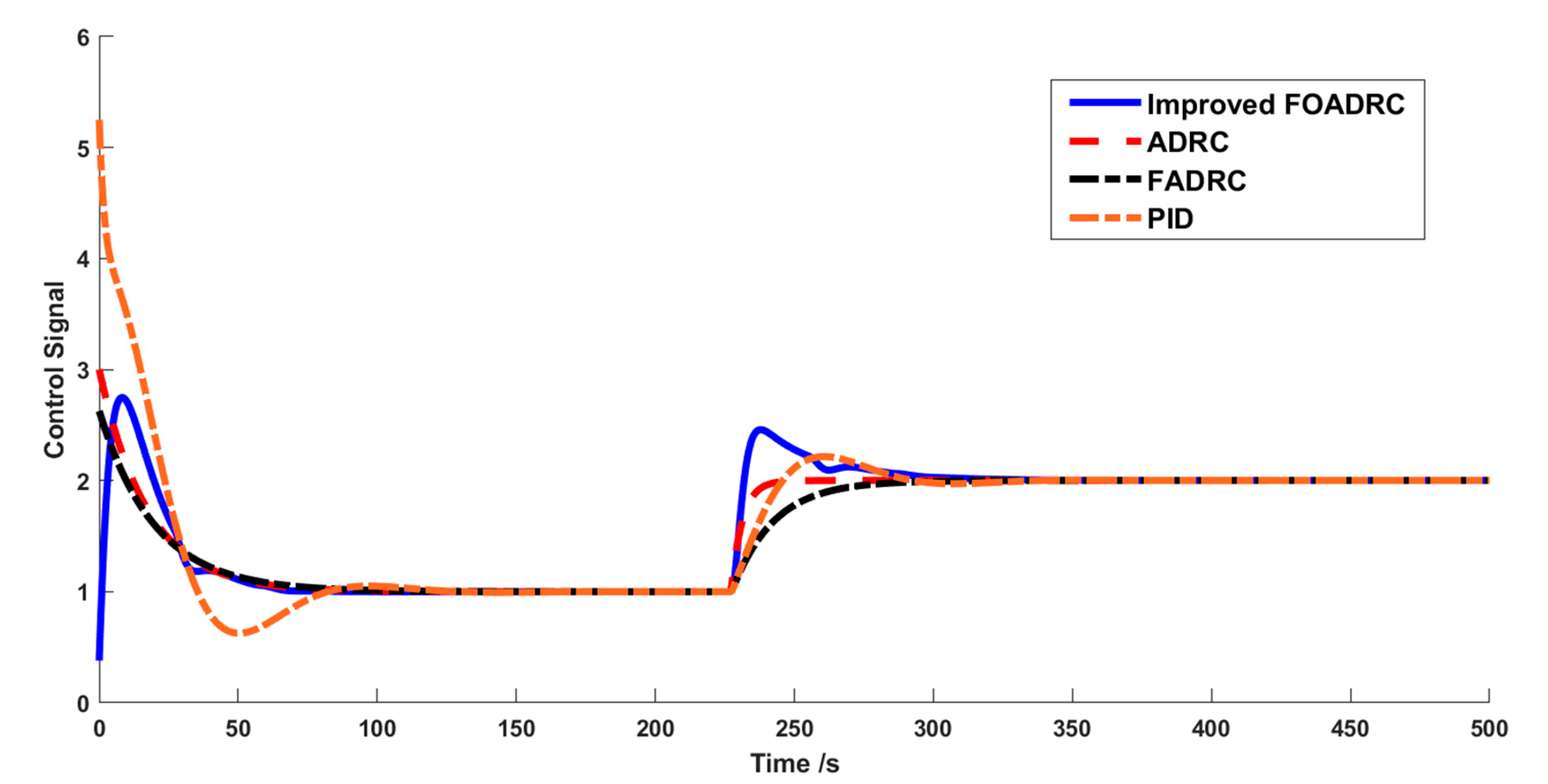
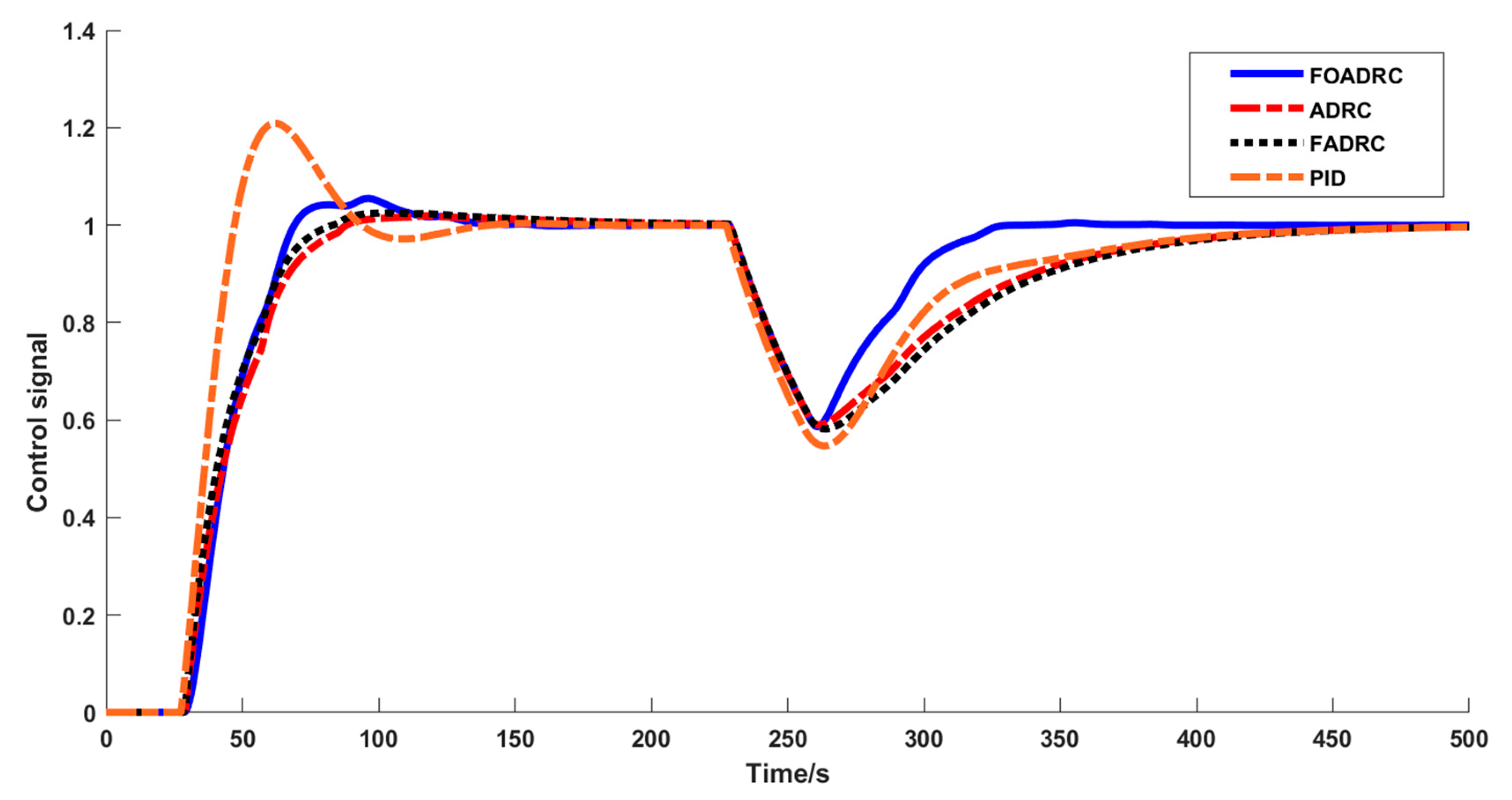
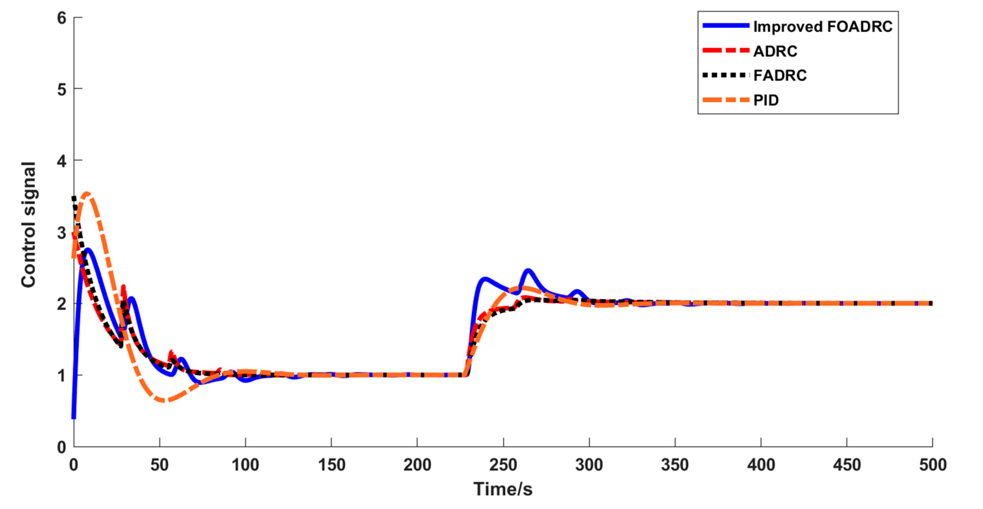
| Control Strategy | IAE | IAE1 | TV | TV1 | Rise Time (s) | Overshoot (%) |
|---|---|---|---|---|---|---|
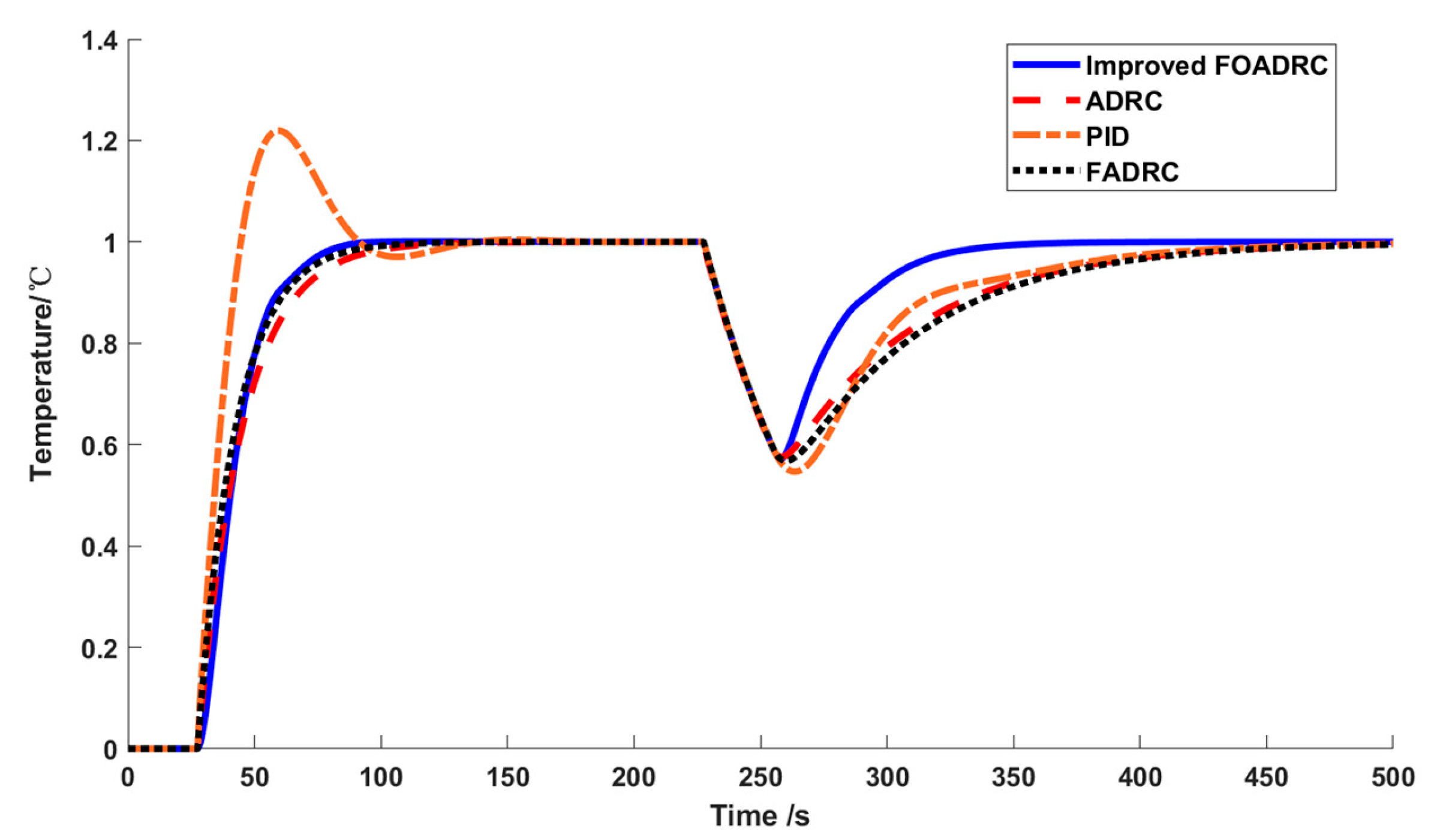
| Improved FOADRC | 42.75 | 43.74 | 1.00 | 1.12 | 35 | 2.2 |
| ADRC | 45.25 | 48.26 | 1.62 | 1.72 | 55 | 3.5 |
| FADRC | 43.75 | 46.56 | 1.12 | 1.30 | 52 | 5.2 |
| PID | 55.23 | 58.45 | 2.21 | 3.14 | 40 | 25 |
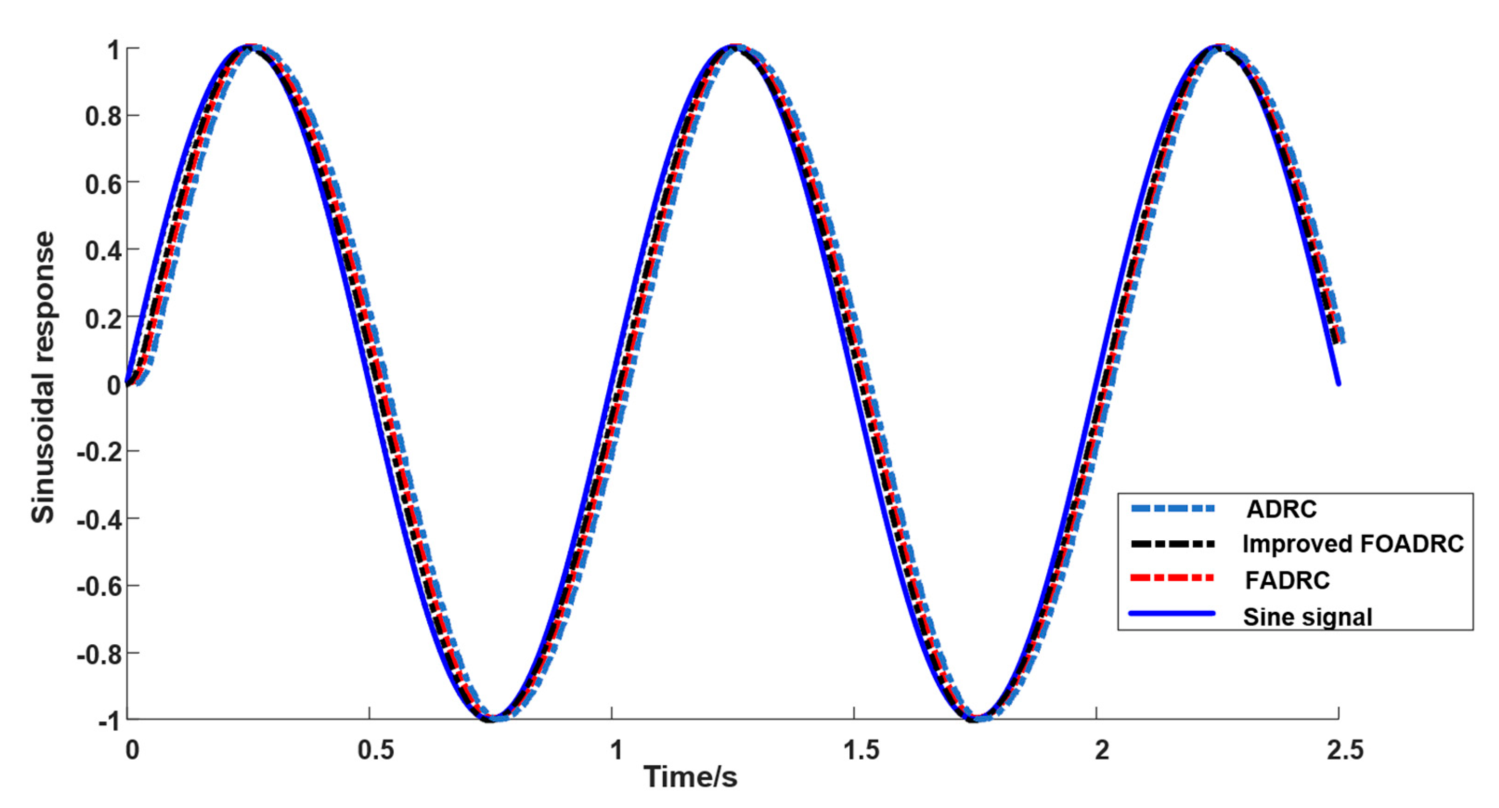
| Control Strategy | Rise Time (s) | Overshoot (%) | Peak Time (s) |
|---|---|---|---|
| Improved FOADRC | 0.18 | 0.2 | 0.24 |
| ADRC | 0.35 | 2.3 | 0.35 |
| FADRC | 0.20 | 1.1 | 0.32 |
Disclaimer/Publisher’s Note: The statements, opinions and data contained in all publications are solely those of the individual author(s) and contributor(s) and not of MDPI and/or the editor(s). MDPI and/or the editor(s) disclaim responsibility for any injury to people or property resulting from any ideas, methods, instructions or products referred to in the content. |
© 2023 by the authors. Licensee MDPI, Basel, Switzerland. This article is an open access article distributed under the terms and conditions of the Creative Commons Attribution (CC BY) license (https://creativecommons.org/licenses/by/4.0/).
Share and Cite
Tang, X.; Xu, B.; Xu, Z. Reactor Temperature Control Based on Improved Fractional Order Self-Anti-Disturbance. Processes 2023, 11, 1125. https://doi.org/10.3390/pr11041125
Tang X, Xu B, Xu Z. Reactor Temperature Control Based on Improved Fractional Order Self-Anti-Disturbance. Processes. 2023; 11(4):1125. https://doi.org/10.3390/pr11041125
Chicago/Turabian StyleTang, Xiaowei, Bing Xu, and Zichen Xu. 2023. "Reactor Temperature Control Based on Improved Fractional Order Self-Anti-Disturbance" Processes 11, no. 4: 1125. https://doi.org/10.3390/pr11041125