Transferring Bubble Breakage Models Tailored for Euler-Euler Approaches to Euler-Lagrange Simulations

Abstract

Most bubble breakage models have been developed for multiphase simulations using Euler-Euler (EE) approaches. Commonly, they are linked with population balance models (PBM) and are validated by making use of Reynolds-averaged Navier-Stokes (RANS) turbulence models. The latter, however, may be replaced by alternate approaches such as Large Eddy simulations (LES) that play a pivotal role in current developments based on lattice Boltzmann (LBM) technologies. Consequently, this study investigates the possibility of transferring promising bubble breakage models from the EE framework into Euler-Lagrange (EL) settings aiming to perform LES. Using our own model, it was possible to reproduce similar bubble size distributions (BSDs) for EL and EE simulations. Therefore, the critical Weber (We_crit) number served as a threshold value for the occurrence of bubble breakage events. We_crit depended on the bubble daughter size distribution (DSD) and a set minimum time between two consecutive bubble breakage events. The commercial frameworks Ansys Fluent and M-Star were applied for EE and EL simulations, respectively. The latter enabled the implementation of LES, i.e., the use of a turbulence model with non-time averaged entities. By properly choosing We_crit, it was possible to successfully transfer two commonly applied bubble breakage models from EE to EL. Based on the mechanism of bubble breakage, We_crit values of 7 and 11 were determined, respectively. Optimum We_crit were identified as fitting the shape of DSDs, as this turned out to be a key criterion for reaching optimum prediction quality. Optimum We_crit values hold true for commonly applied operational conditions in aerated bioreactors, considering water as the matrix.

1. Introduction

Multiphase reactors are intensively used in the chemical and biotech industries. In such (gas–liquid) flow systems, bubble size distribution (BSD) mirrors bubble breakage and coalescence effects. Bubble sizes directly influence hydrodynamic flow and determine the phase exchange area. Consequently, accurate prediction of bubble breakage not only provides a sound basis for precise and comprehensive CFD simulations but also for qualifying mass transfer capacities of a reactor setting. For the calculation of gas–liquid mass transfer between the phases, the Sauter diameter d₃₂ is of particular importance. To predict the dissolved gas concentration gradients within the reactor, the local d₃₂ should be determined as accurately as possible. Often, Euler-Euler approaches are applied considering both the gas and the aqueous phase as a continuum, thereby integrating bubble breakage in population balance models (PBMs). In this context, Reynolds-averaged Navier-Stokes (RANS) turbulence models are commonly applied to finite volume (FV) solvers. Many existing breakage models have been calibrated under these conditions [1,2,3].

Luo et al. [4] probably published the most applied breakage kernel in PBMs. Despite a multitude of alternate approaches, their model continues to be one of the most used frameworks [5,6,7]. In addition, the modified approach of Lehr et al. [1] also gained significance for calculating bubble size distributions [8,9,10]. Interestingly enough, both approaches require the same set of input parameters, namely fluid density, surface tension, turbulence dissipation rate and bubble diameter. As such, they are generally applicable.

Since increasing computational capacities allow the application of sophisticated numerical solvers, the lattice Boltzman (LBM) method has recently been applied to simulate industrial reactors [11,12,13,14]. The approach is well parallelizable, offering the use of modern graphic cards that accelerate computation and that enable treating bubbles as Lagrangian ‘particles’ in Euler-Lagrange (EL) and large eddy (LES) multiphase simulations. The modeling of bubbly flows with the EL framework has received increasing attention in recent years [15,16,17,18]. Typically, the fluid phase is treated as a continuum, while the gas phase consists of a number of tracers that interact with the fluid. Considering all relevant forces, particle movement is calculated by the so-called Verlet integration as described in [19,20] for Lagrangian particles. As LES and EL simulations are computationally demanding, EE comprising RANS turbulence models was the method of choice in the past. However, according to [21], LES simulations of gas–liquid bubble columns achieve better agreement with experimental data than RANS, which integrates the k-$\epsilon$ model. Consequently, our study ultimately aims to make use of its own bubble breakage model as the promising basis for performing LES simulations.

EL simulations of multiphase (bio-)reactors do not require the implementation of PBMs. Instead, breakage conditions are qualified individually for each bubble. Nevertheless, the successful application of the two breakage models of [4] and [1] asks for equal breakage predictions in EE and EL simulations. Considering the main input parameters, fluid density, surface tension, turbulence dissipation rate and bubble diameter, this requirement is hard to achieve, as local turbulence dissipation rates differ significantly in the LES and k-$\epsilon$ context. As a workaround, this study introduces the critical Weber number We_crit, i.e., a critical ratio of fluid inertia versus surface tension, as a pivotal threshold value for starting bubble breakage. This dimensional criterion for bubble breakup, as used in EL contexts, has been documented in several recent investigations [15,17,21,22,23].

We are local numbers that may be easily derived from fluid mechanics, which allows using the original breakage models instead of adapting them [15]. Although the approach may succeed in correctly predicting model breakage events, the forecasting of daughter size distributions (DSD) may still be demanding. In the EE framework, the solution of the integro-differential PBM ensures ‘pseudo’ steady-state bubble size distributions. In the EL framework, DSDs result from the individual analysis of each breakage event, which introduces a stochastic element. Therefore, this study also presents suitable DSD shapes together with their mathematical descriptions.

In essence, the two well-known bubble breakage models, [4] and [1], need to be transferred and validated regarding their application in EL, LES turbulence models and LBM simulations. The goal is to present a bubble breakage description that is applicable for a wide range of datasets and mechanistic bubble breakage effects thanks to the modular structure of critical We number and the consideration of individual DSDs.

2. Materials and Methods

All simulations were performed in a bubble column with a height of 1.3 m and a diameter of 0.2 m, resulting in a total volume of 40.84 L. The identical geometry and operating parameters were chosen for both simulations, EE and EL. The air volume flow rate was kept constant at 4 L min⁻¹ at the ring sparger. To provoke and enhance bubble breakage, the liquid was steadily injected at the center of the bottom and simultaneously removed from the top of the reactor, mimicking an external fluid loop. Both the inlet and outlet tube had a diameter of 24 mm. The volume flow rate varied to expose bubbles to different turbulence intensities. The bubble diameter at the inlet remained at 16 mm. Fluid viscosity, density and surface tension were assumed to be similar to the properties of water. According to [24], the specific energy dissipation rate ${\epsilon }_{pump}$ caused by the pump was calculated directly from the pump volume flow rate $\dot{v}$ in Equation (1):

$${\epsilon }_{pump}=\frac{\frac{1}{2}\dot{v}\rho w^2}{V_l}$$

(1)

In addition to the volume of the bubble column V_l and the liquid density $\rho$, the liquid velocity at the inlet w was considered. The latter was defined as the pump volume flow in relation to the inlet area A in Equation (2):

$$w=\frac{\dot{v}}{A}$$

(2)

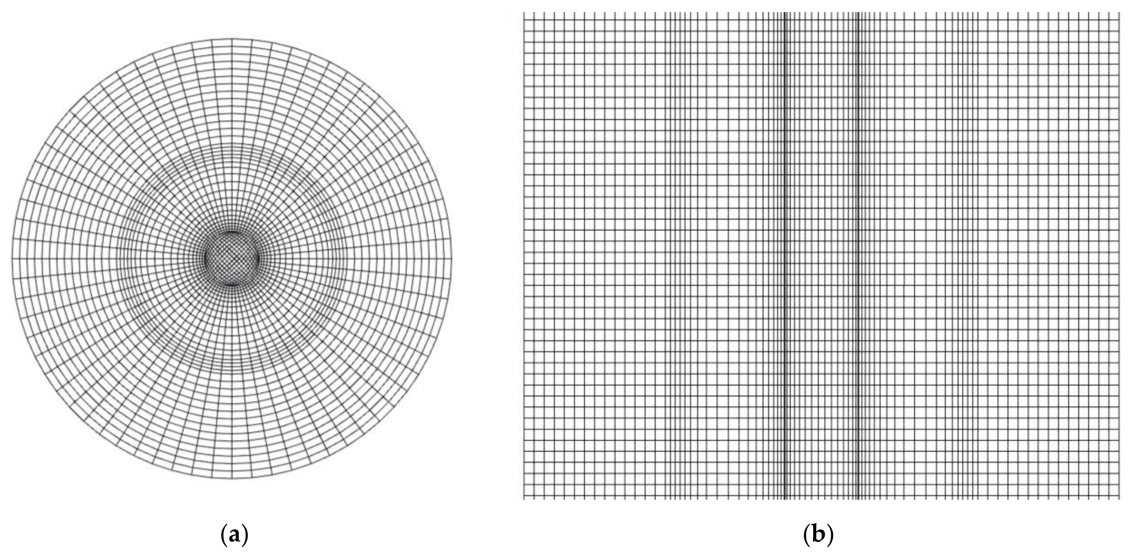
2.1. Bubble Column Simulation in the Euler-Euler Approach

The simulation in the FV approach was performed with Ansys Fluent 2021. The multiphase fluid was realized as EE using a mesh of hexahedrons to enable numerical stability (see Figure 1). Turbulence was modeled with the help of the renormalization group (RNG) k-$\epsilon$ model yielding time-averaged turbulent kinetic energy k and turbulent kinetic dissipation rate $\epsilon$. Notably, the identical turbulence model employed by Lehr et al. [1] was used in this study. After evaluating a mesh independence study with three different mesh densities, the total grid number was set to 862,750. The velocity magnitude was accurately predicted for all mesh densities. However, the peak turbulent dissipation rate was overestimated for the lowest mesh density at a height of 0.2 m, as depicted in Figure 2a. The middle mesh was considered to be sufficiently accurate, offering acceptable computation time. The correlations for the drag coefficient obtained from Tomiyama et al. [25] were embedded in the model. For stability reasons, no further bubble forces have been implemented, as it was assumed that the bubble velocity was dominated by the surrounding fluid movement. With a population balance model (PBM) consisting of 20 discrete size classes, the bubble size distribution (BSD) was sufficiently well resolved. The size classes were distributed applying a growth ratio exponent of 0.5 in the range between 1 and 16 mm. With a timestep of 0.01 s, it was possible to reach the threshold of at least 10⁻⁴ for all residuals. Once the threshold was achieved, steady-state conditions were assumed. The BSD was evaluated only in the upper third of the column, as it was assumed that the bubble breakage process was completed at this position. A summary of all settings is listed in

Table 1. Geometry, simulation set-up, boundary conditions and solver setting of bubble column simulation in Ansys Fluent.

Properties	Boundary Conditions	Units
Fluid inlet	Volume flow: 0.6, 0.9, 1.2, 1.5	L s−1
Air inlet	Volume flow: 4	L min−1
Outlet	Degassing
Wall	No-slip
Initial bubble size	16	mm
Column diameter	0.2	m
Column height	1.3	m
Multiphase	Euler-Euler
Ring sparger diameter	Ring diameter × tube diameter (8.8 × 0.9)	cm
Fluid inlet diameter	24	mm
Population balance model	Discrete with 20 bins in range [1–16 mm]
Breakage model	Luo et al. and Lehr et al.
Turbulence	RNG k-$\epsilon$ model
Phase interactions
	Drag	[25]
Solution methods
Pressure-velocity coupling	Phase coupled SIMPLE
Gradient	Least Squares Cell Based
Pressure	Body Force Weighted
Momentum	QUICK
Volume fraction	QUICK
Turbulent kinetic energy	Second Order Upwind
Turbulent dissipation rate	Second Order Upwind
Phase-2 Bin	Second Order Upwind
Transient Formulation	Bounded Second Order Implicit
Time step size	0.01	s
Total mesh size	862,750

.

2.2. Bubble Column Simulation in the Euler-Lagrange Approach

For the LES simulations using the lattice Boltzmann method, the commercial software M-Star CFD 3.2.6 (https://mstarcfd.com (accessed on 10 November 2022)) was applied. According to the D3Q19 velocity vector set, the 3D space is discretized into equally distributed grid points with predefined distance. Every grid point is surrounded by 19 direct neighbors, incorporated by the ith orientation of vector c_i. Each point is individually defined by the probability density function $f_i\left(x,t\right)$, representing fictitious parcels as a proxy for fluid movement. The LB algorithm consists of two steps: collision and streaming. During the streaming step, the parcels move with a constant velocity from node to node, each providing updating information after the respective time step Δt. The model presumes that the fluid relaxes locally to the equilibrium distribution function $f_i^{eq}\left(x,t\right)$ over a characteristic timescale $\tau$, which depends on the molecular viscosity of the fluid. In the standard LBM equation, the collision step is described on the right-hand side in Equation (3) [26,27].

$$\frac{f_i\left(x+c_i\Delta t,t+\Delta t\right)-f_i\left(x,t\right)}{\Delta t}=-\frac{1}{\tau }\left[f_i\left(x,t\right)-f_i^{eq}\left(x,t\right)\right]$$

(3)

whereas the microscopic scale is simplified, the macroscopic scale can be described with second-order accuracy. The operations of the right and left sides of Equation (3) may be easily parallelized, which allows computation on a graphic processor. All walls were considered as no-slip surfaces. To remove the bubbles, the fluid column was defined as a free surface boundary condition at the top. Analogous to the EE approach, the drag force was derived using the correlation of [25] to calculate the drag force coefficient. It was assumed that the effect of other forces on bubble motion was negligible. However, it was evident that lift force stabilizes the bubbles horizontally, so the implementation of the lift coefficient of [28] turned out to be beneficial. The LES model was used to take turbulence into account. Numerous studies have demonstrated the superior precision of LES simulations over RANS turbulence models [21,29,30,31]. The use of LES methods as the standard for LBM simulations is justified by the potential to apply greatly parallelized algorithms [12,13,18]. Eddies below the sub-grid scale were incorporated with the Smagorinsky model [32] by calculating the sub-grid eddy viscosity ${\nu }_t$ with Equation (4):

$${\nu }_t={\left(C_S{\Delta }_x\right)}^2\left|\overline{S}\right|$$

(4)

The Smagorinsky coefficient $C_s$ was kept to 0.1, which is the default value in M-Star. Additionally, ${\nu }_t$ depends on the grid size ${\Delta }_x$ and the filtered strain rate tensor $\overline{S}$. The accuracy and quality of a LES are strongly linked to the mesh density. With finer grid resolution, a broader spectrum of eddy sizes can be resolved. This effect can be seen in the mesh independence study shown in Figure 2b. When comparing three different mesh densities, the turbulence dissipation rate was overestimated between a column height of 0.01 and 0.2 m, with the lowest grid density of 17.8 M. At a grid density of 24.1 M, the changes of $\epsilon$ were minor compared to the highest resolution and therefore this mesh was chosen for all ongoing simulations. In order to accurately assess the impact of turbulence on bubble breakage, it is essential to ensure precise reproduction of $\epsilon$ for all reactor heights.

In the framework of the EL approach, it is recommended that bubble diameters be at least an order of magnitude smaller than the mesh spacing to ensure that the impulse between the bubble and the fluid is accurately transferred [33]. Interestingly, Sungkorn et al. [18] suggested that minimal numerical mesh sizes double the bubble diameter were sufficient. However, none of those criteria were applied in the present work, as bubbles are larger than the grid spacing for the sake of high fluid resolution. Accordingly, it was assumed that the bubble-induced fluid movement was underestimated with the current approach. In the current application, this bias was of minor importance since the flow field was dominated by the convective flow of the recirculation pump. Notably, this simulation setting was chosen as it was the pivotal interest of this study to investigate the interaction of $\epsilon$ with bubbles.

The BSD was evaluated at a column height between 0.95 and 1.15 m. At this height, no further bubble breakage occurred. After 10 s, a pseudo-equilibrium was established, so that the evaluation was carried out for an additional 10 s in each case. The state of each bubble was recorded every 0.01 s. A lattice time step size $\Delta t$ between 3 × 10⁻⁶ and 1.6 × 10⁻⁵ s kept lattice density deviation below 2% (usually significantly lower). A summary of all settings is listed in

Table 2. Geometry, simulation set-up, boundary conditions and solver setting of bubble column simulation in M-Star.

Properties	Boundary Conditions	Units
Fluid inlet	Volume flow: 0.6, 0.9, 1.2, 1.5	L s−1
Air inlet	Volume flow: 4	L min−1
Outlet	Free Surface
Wall	No-slip
Initial bubble size	16	mm
Column diameter	0.2	m
Column height	1.3	m
Ring sparger diameter	Ring diameter × tube diameter (8.8 × 0.9)	cm
Fluid inlet diameter	24	mm
Multiphase	Euler-Lagrange
Breakage model	Modified Weber number
Turbulence	LES
	Sub-grid model	[32]
	Smagorinsky coefficient	0.1
Phase interactions
	Drag	[25]
	Lift	[28]
Fluid-bubble coupling	Density
Velocity vector set	D3Q19
Time step size	Between 3 × 10−6 s and 1.6 × 10−5 s	s
Total mesh size	24.1 M

.

2.3. Bubble Breakage Models for the Euler-Euler Approach

The models of Luo et al. [4] and Lehr et al. [1] differ in the formulation of the force balance equation. Luo et al. assumed that the hitting eddy transfers more energy than needed to merge the cells, which would lead to an increased bubble surface. The criterion of Lehr et al. [1] compares interfacial forces with external stress by the eddies and considers breakup if the latter exceeds the interfacial stability. The breakup of a bubble is caused by the hydrodynamic conditions in the surrounding fluid and by individual bubble properties. A detailed review of bubble breakage models may be found in [34], indicating that turbulent fluctuations and bubble-to-eddy collisions are the dominating factors for breakage. As bubbles interact with turbulent eddies, they exchange energy and momentum with the fluid, resulting in interfacial instabilities. Once the stabilizing effects by inertia and surface tension are smaller, bubble breakage occurs. In EE applications, a breakup kernel function is usually defined as:

$${\mathsf{\Omega }}_B\left(V:V^{\prime }\right)={{\displaystyle \int }}_{{\lambda }_{\min }}^{{\lambda }_{\max }}{\omega }_B\left(V\right)P_B\left(V,V^{\prime }\right)d\lambda$$

(5)

Here, ${\omega }_B\left(V\right)$ is the frequency of eddies of length scale between $\lambda$ and $\lambda +d\lambda$ hitting the bubble, and $P_B\left(V,V^{\prime }\right)$ is the probability that said bubble breaks into two smaller parts, if sufficient turbulent energy is provided. The volumes of the parent and daughter bubbles are denoted by V and V’, respectively. The collision frequency ${\omega }_B\left(V\right)$ for the model Luo et al. [4] may be determined in analogy to kinetic gas theory and depends on the bubble diameter d and the number density of bubbles.

For the final description of ${\mathsf{\Omega }}_B\left(V:V^{\prime }\right)$ in Equation (6), the equations for ${\omega }_B\left(V\right)$ and $P_B\left(V,V^{\prime }\right)$ are inserted into (5):

$${\mathsf{\Omega }}_B\left(V:V^{\prime }\right)=0.9238{\epsilon }^{\frac{1}{3}}{d}^{-\frac{2}{3}}\alpha {{\displaystyle \int }}_{{\xi }_{min}}^1\frac{{\left(1+\xi \right)}^2}{{\xi }^{11/3}}{e}^{-12\left(f_V^{\frac{2}{3}}+{\left(1-f_V\right)}^{\frac{2}{3}}-1\right)\sigma \beta {\rho }^{-1}{\epsilon }^{-\frac{2}{3}}{d}^{\frac{5}{3}}{\xi }^{-\frac{11}{3}}}d\xi$$

(6)

The model, according to Lehr et al. [1], employs equivalent formulations for ${\omega }_B\left(V\right)$. However, the breakage probability is obtained from the balance between bubble surface tension and the interfacial force of the hitting eddy. The former explicitly refers to the surface tension of the smaller bubble. For this purpose, the velocity spectrum around the mean value is considered, which can be assumed to be normally distributed [35]:

The final breakage frequency ${\mathsf{\Omega }}_B\left(V:V^{\prime }\right)$ is formulated in Equation (7).

$${\mathsf{\Omega }}_B\left(V:V^{\prime }\right)=1.19{\epsilon }^{\frac{-2}{3}}{d}^{-\frac{2}{3}}\sigma {\rho }^{-1}{f}_V^{-\frac{1}{3}}{{\displaystyle \int }}_{{\xi }_{\min }}^1\frac{{\left(1+\xi \right)}^2}{{\xi }^{\frac{13}{3}}}\exp \left(-2\sigma {\rho }^{-1}{\epsilon }^{-\frac{2}{3}}{d}^{-\frac{5}{3}}{f}_V^{-\frac{1}{3}} {\xi }^{-\frac{2}{3}}\right)d\xi$$

(7)

Lehr et al. were able to provide an analytical solution without the integral in Equation (8), which was very helpful when considering Lagrangian particles.

$${\mathsf{\Omega }}_B\left(V:V^{\prime }\right)=0.5\frac{d_i^{\frac{5}{3}}{\epsilon }^{\frac{19}{15}}{\rho }^{\frac{7}{5}}}{{\sigma }^{\frac{7}{5}}}\exp \left(-\frac{\sqrt{2}{\sigma }^{\frac{9}{5}}}{d_i^3{\rho }^{\frac{9}{5}}{\epsilon }^{\frac{6}{5}}}\right)$$

(8)

The work of Luo et al. [4] and Lehr et al. [1] limited the integration on the turbulence wavenumber such that only eddies smaller or equal to the bubbles may cause their breakage. In both cases, only binary bubble breakage is considered.

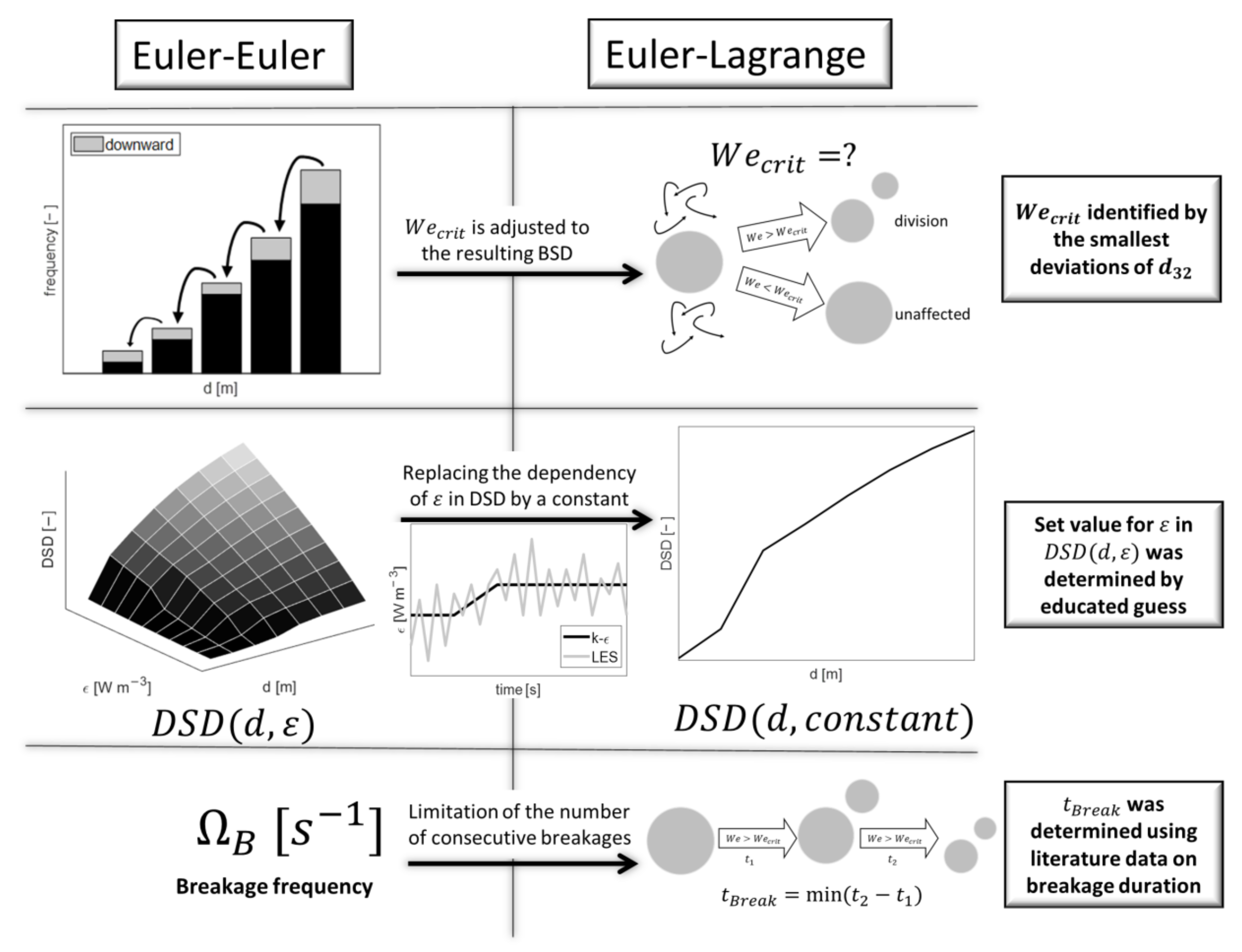
2.4. Bubble Breakage Model Description for the Euler-Lagrange Approach

A crucial limit for the occurrence of breakage in EL is formulated by comparing the disruptive and cohesive stress of the bubble, as it is done by the We number (Equation (9)), a dimensionless number describing fluid’s inertia compared to its surface tension $\sigma$.

$$We=\frac{\rho u^{2}d}{\sigma }$$

(9)

Under the action of viscous shear, a drop elongates into the shape of a prolate ellipsoid. If the exposed energy force exceeds a critical value, the bubble breaks.

$$We=\frac{\rho \delta u^2\left(d\right)d}{\sigma }$$

(10)

In turbulent flows, the deformation is induced by $\delta u^2\left(d\right)$ which is the mean square velocity difference over a distance equal to d. Kolmogorov [36] postulated that the criteria becomes independent of viscosity if the Reynold number is high enough. Assuming isotropic turbulence, $\delta u^2\left(d\right)$ can be replaced by the dominant hitting eddy influence in Equation (10).

$$We=\frac{\rho \beta {\left(\epsilon d\right)}^{\frac{2}{3}}d}{\sigma }=\frac{\rho \beta {\epsilon }^{\frac{2}{3}}{d}^{\frac{5}{3}}}{\sigma }$$

(11)

The model constant $\beta$ in Equation (11) varies throughout the literature and is measured with a value of 2 according to [37], which is offset against the critical Weber number We_crit. Since $\rho$ and $\sigma$ are assumed to be constant during the simulation, $\epsilon$ and d are the crucial parameters for breakage. These influencing variables are also decisive in the original models. A critical We number needs to be found in such a way that it is able to reproduce the bubble breakup rates of the considered models. For bubble breakage, the condition of Equation (12) applies:

$$W{e}_{crit}<We$$

(12)

The number of breakage events increases with increasing bubble diameter and turbulent dissipation rate. Notably, only these local parameters affect bubble breakage but not the experimental setting that is used for creating the breakage scenario. In our study, all simulations were performed for a water–air system. However, the presented kernels are functions of surface tension and fluid density. Therefore, they are transferable to liquids with changed physical properties.

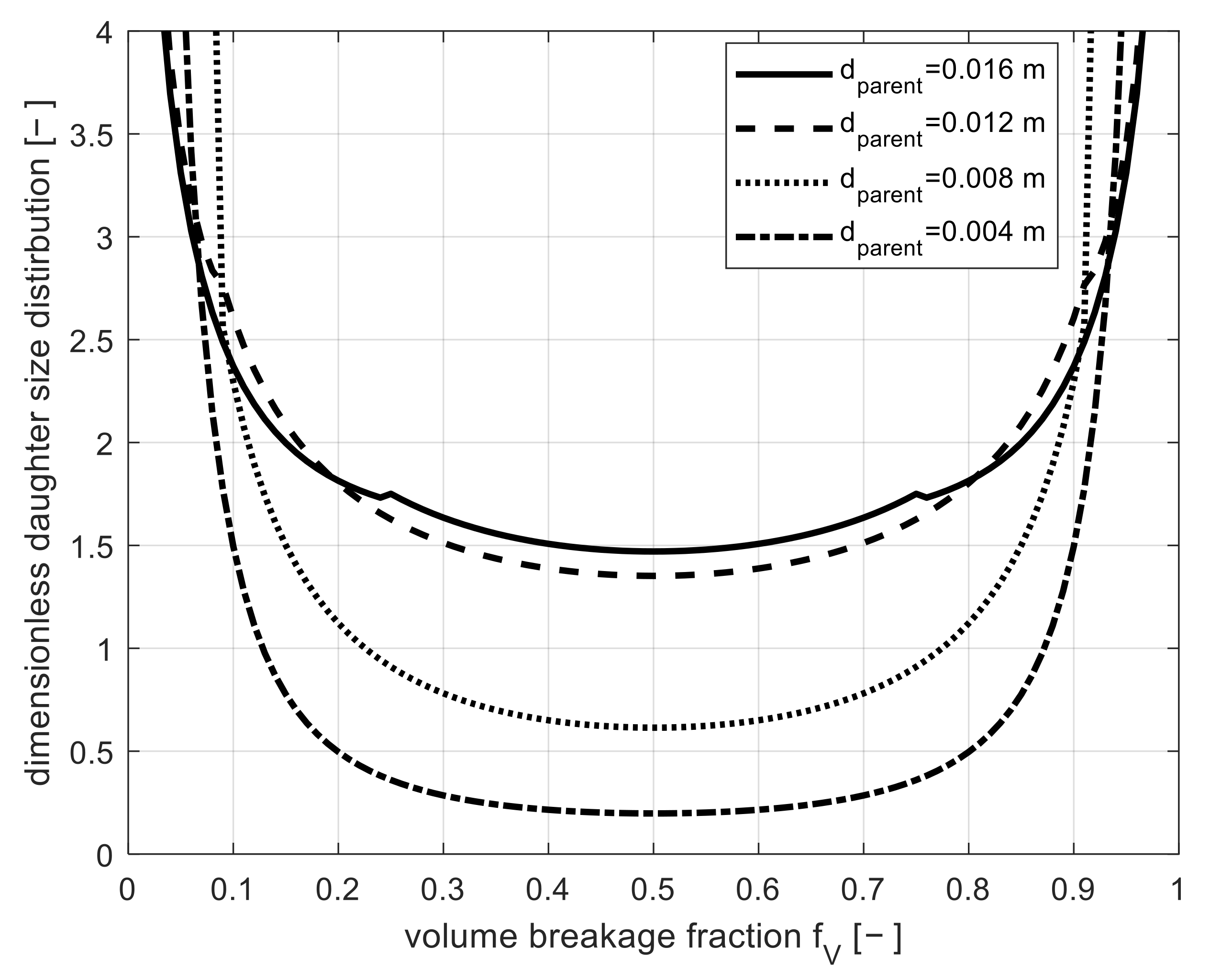
2.5. Daughter Size Distribution for Bubble Breakage Models

In addition to the breakup frequency, the size of the two generated daughter bubbles must be known. In [34], different types of DSD formulations are categorized. The distributions of [4] and [1] are formulated as algebraic expressions, finally creating either bell-, U- or M-shape daughter bubbles. Hesketh et al. [38] experimentally showed that equal breakup is unlikely because more energy is required to outplay the increased surface tension of equal bubbles compared to non-equal bubbles. Since only binary splitting is considered, the distribution has to be symmetric. This results in a U-shape of the distribution with a global minimum at $f_V$ = 0.5. The DSD used by [4] is created by normalizing the breakup frequency by the overall breakage frequency, as seen in Equation (13).

$$DSD\left(d_j,d_i\right)=\frac{{\mathsf{\Omega }}_B\left(V:V^{\prime }\right)}{{\mathsf{\Omega }}_B\left(V\right)}$$

(13)

This model causes a high probability of daughter bubbles close to zero and one. The DSD in the U-shape is formulated in its final form according to Luo et al. in Equation (14):

$$DSD\left(d_j,d_i\right)=\frac{2{{\displaystyle \int }}_{{\xi }_{min}}^1\frac{{\left(1+\xi \right)}^2}{{\xi }^{\frac{11}{3}}}{e}^{-12\left(f_V^{\frac{2}{3}}+{\left(1-f_V\right)}^{\frac{2}{3}}-1\right)\sigma \beta {\rho }^{-1}{\epsilon }^{-\frac{2}{3}}{d}^{\frac{5}{3}}{\xi }^{-\frac{11}{3}}}d\xi }{{{\displaystyle \int }}_0^1{{\displaystyle \int }}_{{\xi }_{min}}^1\frac{{\left(1+\xi \right)}^2}{{\xi }^{\frac{11}{3}}}{e}^{-12\left(f_V^{\frac{2}{3}}+{\left(1-f_V\right)}^{\frac{2}{3}}-1\right)\sigma \beta {\rho }^{-1}{\epsilon }^{-\frac{2}{3}}{d}^{\frac{5}{3}}{\xi }^{-\frac{11}{3}}}d\xi d{f}_V}$$

(14)

Lehr et al. [1] provided a separate function for $DSD\left(d_j,d_i\right)$ which is rooted on a lognormal distribution:

$$DSD\left(d_j,d_i\right)=\frac{1}{\sqrt{\pi }{f}_V}\frac{\exp \left(-\frac{9}{4}{\left(\ln \left(\frac{2^{\frac{2}{5}}{d}_j{\rho }^{\frac{3}{5}}{\epsilon }^{\frac{2}{5}}}{{\sigma }^{\frac{3}{5}}}\right)\right)}^2\right)}{1+\mathrm{e}rf\left(\frac{3}{2}\left(\ln \left(\frac{2^{\frac{1}{15}}{d}_i{\rho }^{\frac{3}{5}}{\epsilon }^{\frac{2}{5}}}{{\sigma }^{\frac{3}{5}}}\right)\right)\right)}$$

(15)

The DSD of [1] is basically characterized by an M-shape, with a local minimum at $f_V$ = 0.5, thereby preferring non-equally sized daughter bubbles. The conditions for M-shaped daughter size distribution are typically observed. However, deviations of the M-shape may occur in the following extreme scenarios: If parent bubbles are small and interfacial forces are high, a bell-shape occurs with a maximum at $f_V$ = 0.5. In contrast, if parent bubbles are large, unequal breakage is preferred and a U-shape is ultimately created.

For each bubble breaking event, an equally distributed random number between 0 and 0.5 is created. The random number is then distorted according to a given function. In [18] and [17], the U-shape of [4] is created by using a tanh or gamma function. These algebraic expressions lead to rigid functions without dependency on d. For this, Equations (14) and (15) were solved directly for each bubble breakage event. First, the integral of the Luo et al. DSD was solved. This was done with the help of an analytic solution based on the gamma function. The gamma function was approximated by the fitting parameters. For Lehr et al., the analytic solution was already available in Equation (15). With a step size of 0.01, a probability was determined for each $f_V$ from 0.01 to 0.99. The original equally distributed random number was then distorted accordingly. In comparison to RANS, $\epsilon$ was not time-averaged when calculated with the LES turbulence model. As can be seen in Figure 2, $\epsilon$ was therefore one order of magnitude larger. The influence of $\epsilon$ on the original DSD was smaller compared to d, as indicated by the exponents in (14) and (15). The effect of $\epsilon$ on DSD was therefore neglected entirely by replacing it with a constant. Details are given in Appendix B. The software code for implementation in M-Star can be found in Supplementary Materials.

2.6. Bubble Breakage Duration

In an EL framework, it must be ensured that a bubble can only break once within a time step to prevent a cascade of breakage events in high turbulence areas. The parameter $t_{Break}$ defines the minimum time between two consecutive bubble breakage events and thus limits the number of successive separations. A proxy for the time scale of this parameter is the duration of the breakage process of a single bubble. First, the bubbles undergo unstable oscillations before stable daughter bubbles are created after division. According to [39], the breakage time may be estimated by the motion of two fractions of fluid in a turbulent flow field and is therefore proportional to $\epsilon$. The bubble diameter is the characteristic length along the turbulent fluctuations. Therefore, it can be written:

$$t_{Break}=0.5{\epsilon }^{-\frac{1}{3}}{d}^{\frac{2}{3}}$$

(16)

Both deformation and breakage times of drops were measured with high-speed movie cameras in different experiments [38,40,41]. When transferring bubble breakage models from the EE to the EL approach, $t_{Break}$ is an important fitting parameter, as this factor must be found in such a way that the model is valid in a wide turbulence spectrum. With a large value for $t_{Break}$, over-proportional breaking can be prevented in highly turbulent regions.

2.7. Bubble Size Distribution Evaluation

In summary, the bubble breakage description for an EL approach consists of the optimized We_crit, the minimum time between two bubble breakages and a suitable DSD. The related parameters must be found individually for each scenario and are only valid for the given setting. In our study, the quality of the fitted solution was evaluated based on multiple criteria. The Sauter diameter d₃₂ weights the size classes and is influenced by the shape of the overall distribution, as shown in Equation (17).

$$d_{32}=\frac{{{\displaystyle \sum }}_{i=1}^{\infty }{d}_i^3}{{{\displaystyle \sum }}_{i=1}^{\infty }{d}_i^2}$$

(17)

3. Results and Discussion

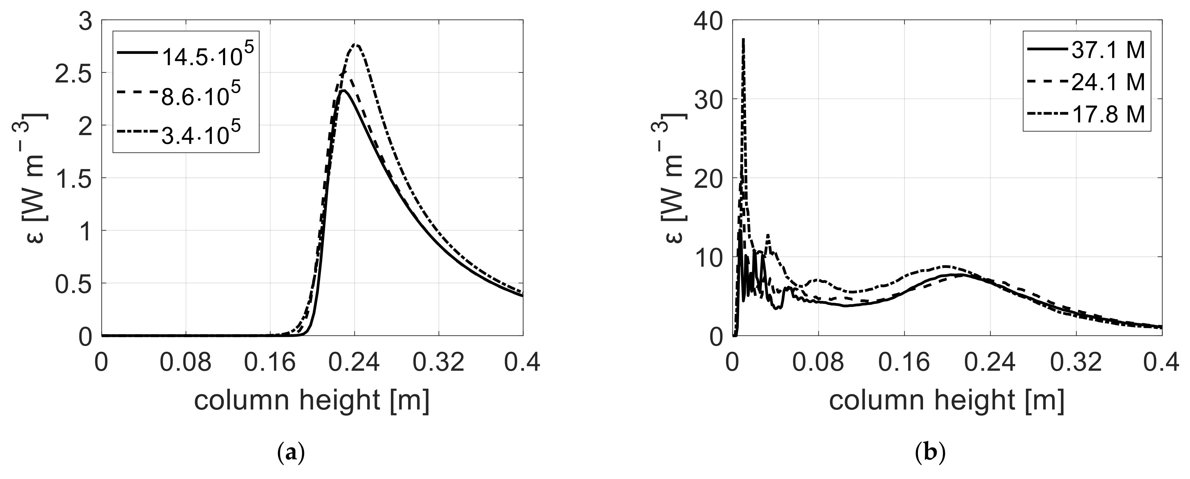
3.1. Influence of the Turbulence Model

Figure 3a,b depict contour plots of $\epsilon$ using FV and LBM, respectively. In both cases, the plane is placed in the center of the column and spans the height from the inlet to the outlet. As indicated, the fluid field is dominated by the convective flow at the inlet. Bubble breakage occurs only in the region of pump-induced turbulence. Since the added liquid is simultaneously removed at the top, the superposed flow directs upward unidirectional with the bubble movement. At the inlet, the fluid movement is concentrated in the column center and slightly disperses with rising column height, finally becoming entirely dispersed. There, upward motions transform into vortices and dissipate, creating small high-energy eddies. The air sparger is located a few centimeters above the pump inlet. Interestingly, bubbles rather escort the main flow field up to 30 cm, where they start experiencing velocity gradients and different intensities of $\epsilon$.

Characteristics of FV performance have been discussed intensively [29,30,31], outlining substantial deviations of said k-$\epsilon$ approach compared to LES in LBM simulations. Comparing Figure 3a,b, those differences become obvious. The key distinction is the time averaging of $\epsilon$ in the k-$\epsilon$ model which is not performed in LES. Such a ‘pseudo’ steady-state solution is shown in Figure 3a. As indicated, $\epsilon$ values that act on the bubbles depend on their position, i.e., those close to the center of the column tend to break more frequently, as local $\epsilon$ values are higher. In contrast, Figure 3b only provides a snapshot of the very dynamic fluid field that constrains bubble breakage to discrete events when bubbles are hit by strong eddies.

Figure 3a shows that there is almost no turbulence predicted by FV, whereas a different scenario is depicted in Figure 3b using LBM. Regarding FV, most bubble breakage occurs in the lower half of the column, whereas LBM identifies upward eddies that may also lead to bubble breakage in higher regions.

The large differences in the resulting contour plots demonstrate that successful transfer of bubble breakage models that are usually applied in EE applications is only possible based on solved fluid fields. Then, the impacts of local eddies on bubble sizes may be additionally considered.

3.2. Describing Daughter Size Distribution (DSD) for the Euler-Lagrange Approach

The current study aimed to find simulation settings that enable the use of the established models by Luo et al. [4] and Lehr et al. [1], not only for EE but also for EL simulations. Consequently, the shapes of DSDs should remain, but proper parameters for EL need to be identified. In the case of the Luo et al. model, this was achieved by a fit function (see Appendix B). Figure 4 and Figure 5 depict the DSD distributions obtained by Equations (14) and (15), respectively. As depicted, varying probabilities for the corresponding $f_V$ are observed. As seen in Figure 6, the DSD shape only changed depending on the parent bubble diameter. As local $\epsilon$values differ (see Figure 3a,b), a constant value for $\epsilon$ had to be found to represent the fluid field over a wide spectrum of turbulence to finally create similar DSD shapes. In the column section of the FV simulation for bubble breakage, the average $\epsilon$ ranges from 0.036 W m⁻³ to 0.446 W m⁻³, depending on the pump energy input. Therefore, constant $\epsilon$ values were set for Luo et al. as 0.08 W m⁻³ and for Lehr et al. as 0.1 W m⁻³. These $\epsilon$ settings enabled the creation of the characteristic distributions, as depicted in Figure 4 and Figure 5. Regarding the approach of [4], there is still a non-zero minimum at $f_V$= 0.5. Equal breakup, however, becomes more likely with rising d_parent. As expected, the distribution of Lehr et al. transforms from a bell, via M to U-shape, with increasing d_parent. For a d_parent of 4 mm or smaller, similar-sized daughter bubbles are most likely.

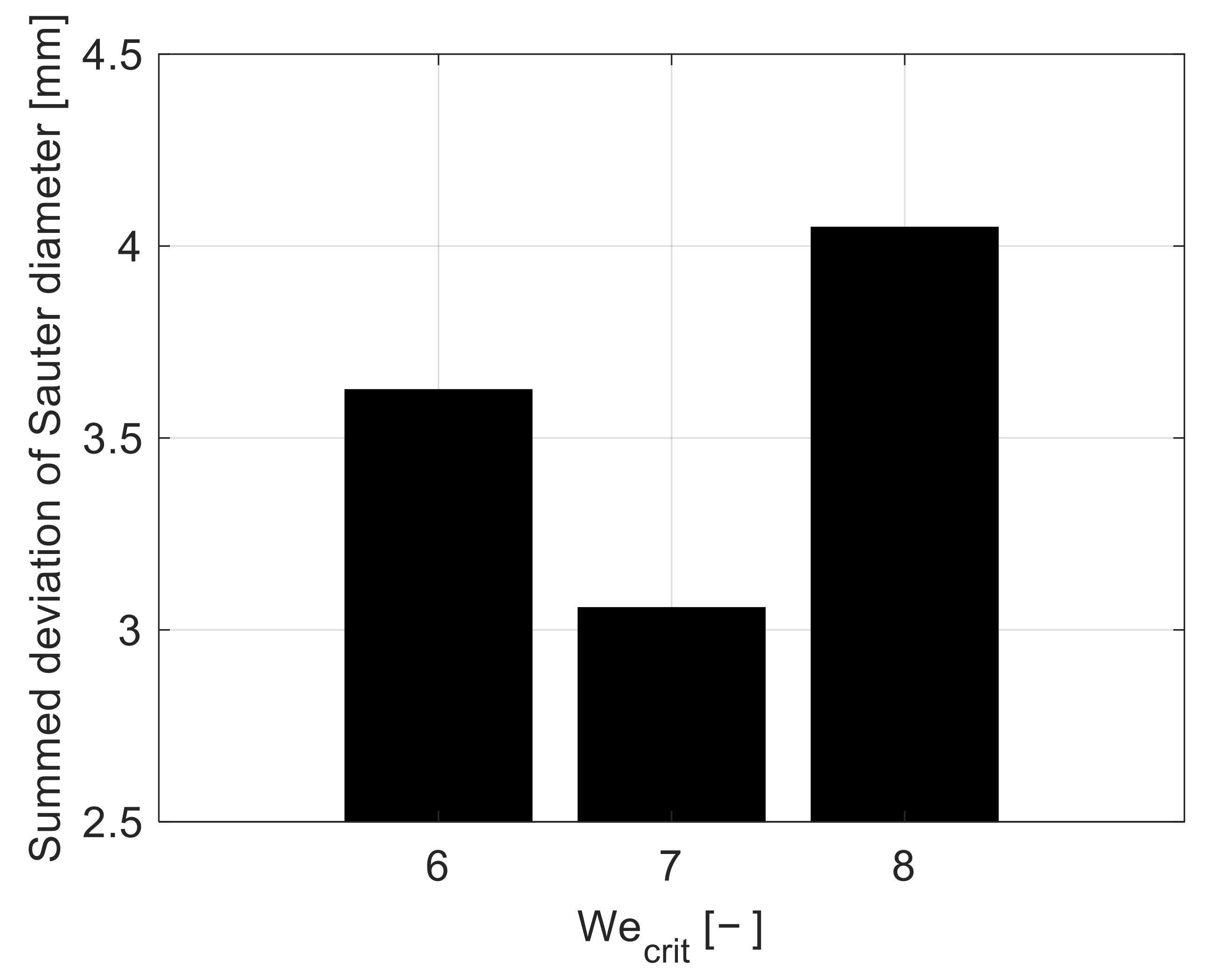
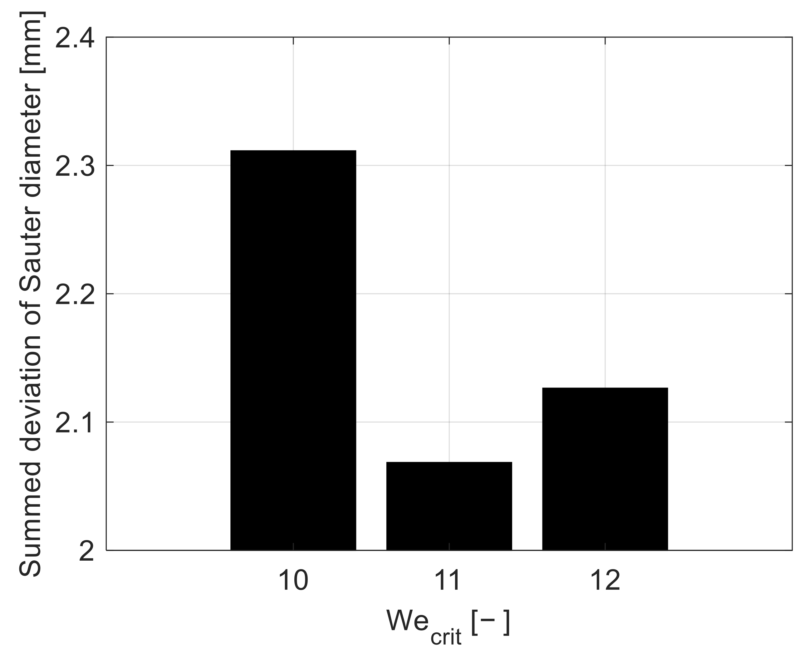
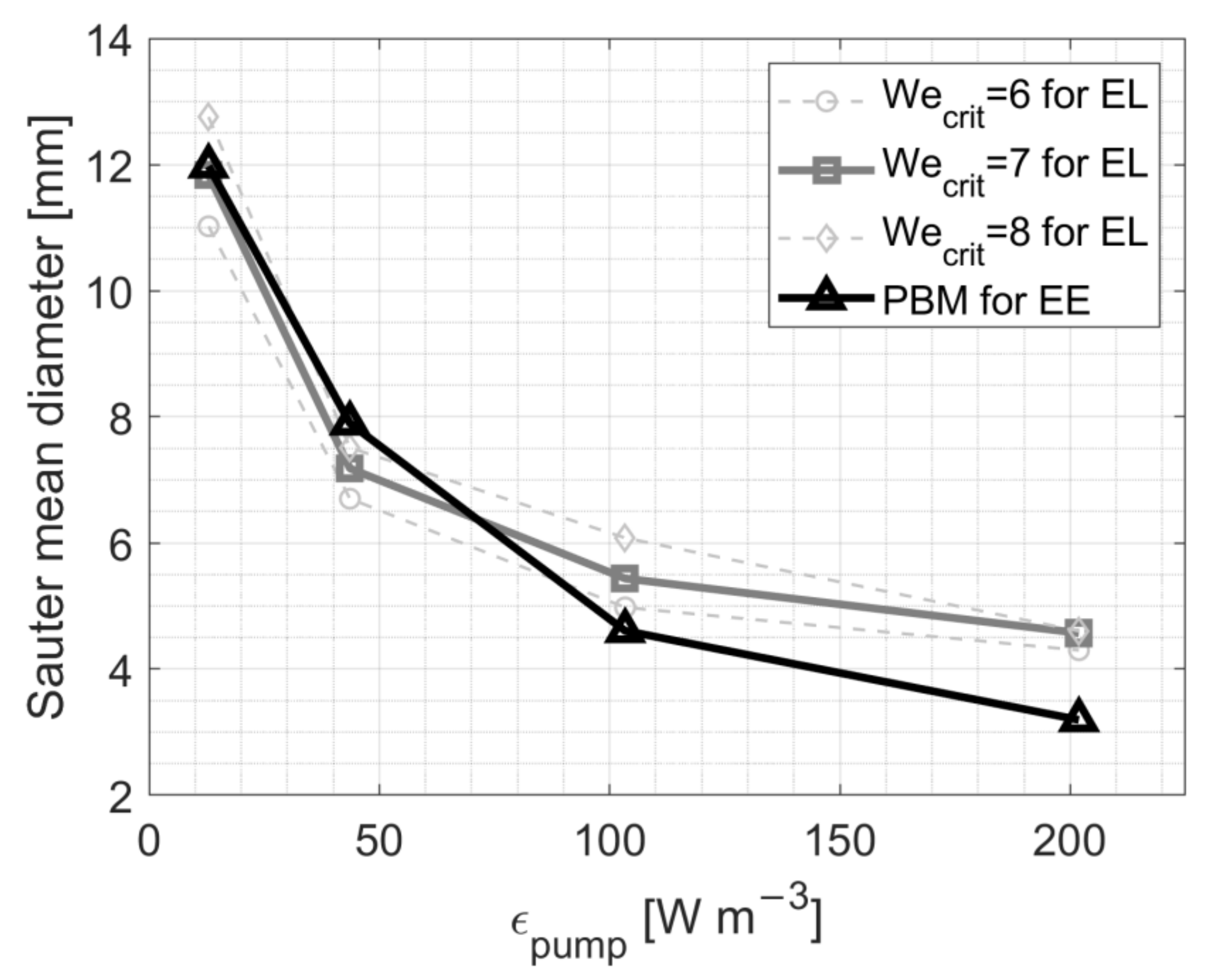
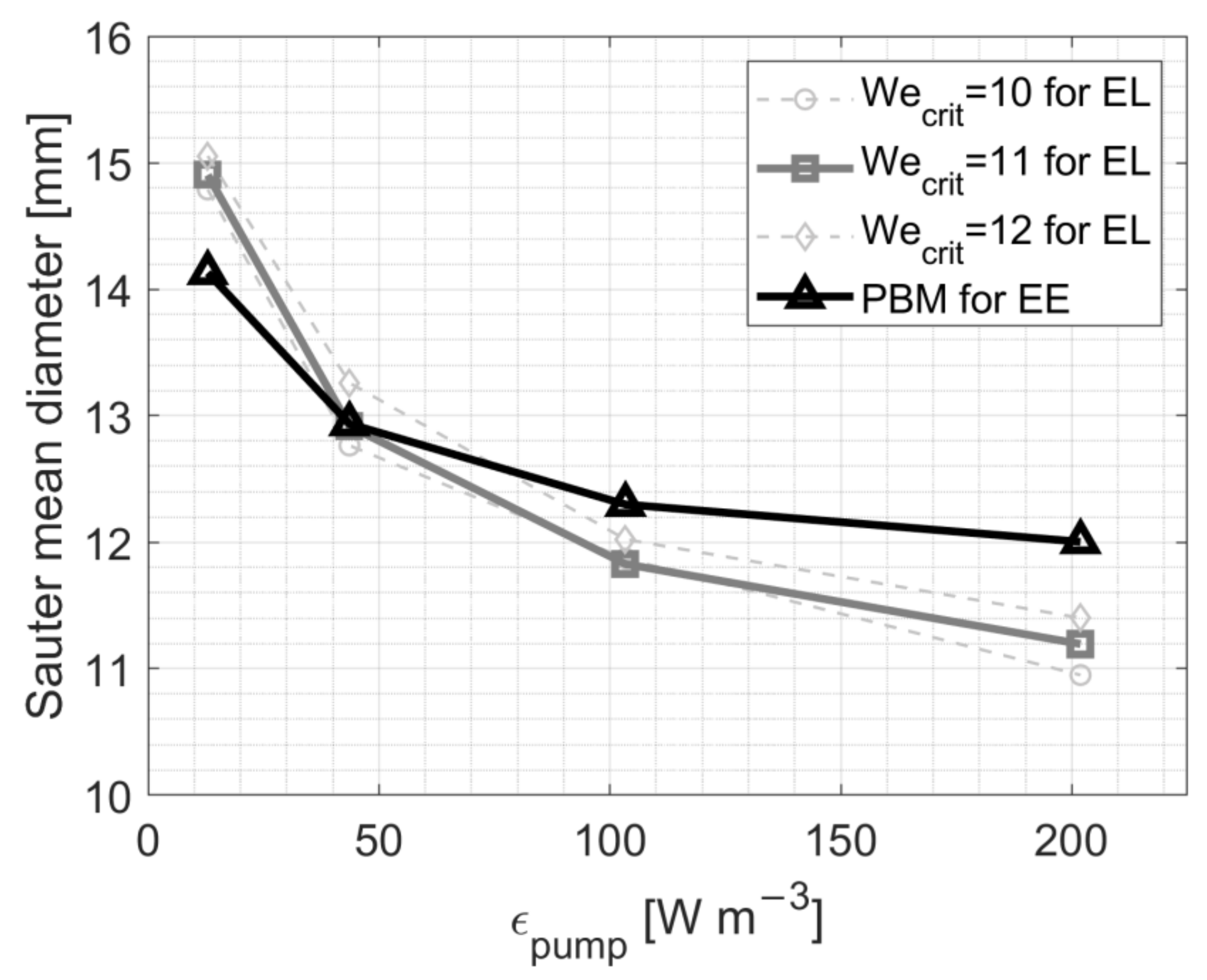
3.3. Optimal Critical We Number and Setting of $t_{Break}$

In addition to the DSD, the parameters $t_{Break}$ and $W{e}_{crit}$ had to be determined. The functionality of the parameters and the method of evaluation are shown in Figure 6. The values for $t_{Break}$ for Luo et al. and Lehr et al. were set to 10 and 250 ms, respectively. In previous studies, a timespan between 3 and 60 ms was experimentally identified for the duration of bubble breakage [40,41,42]. Hence, the duration of 10 ms for the approach of Luo et al. fits in this range. In contrast, the period of 250 ms set for the model of Lehr et al. model is relatively high, reflecting the timespan of breakage of a single bubble. Lehr et al. [1] validated their model based on the experimental findings of [43,44], in which they studied the breakup of air bubbles in a turbulent water jet. Bubbles were injected into the core of the jet, and the spatial evolution of the BSD was measured. Shuai et al. [40] described the effect that if the daughter bubble undergoes a transport process during breakup, the duration is significantly longer, leading to a timespan between 1000 and 2500 ms. Luo et al. [4] validated their model based on experiments of [38] in which no jet flow was involved and thus no transport process associated. It is therefore reasonable to identify a significantly longer $t_{Break}$ for Lehr et al. According to Equation (16), it can be deduced that the individual duration of bubble breakage depends on ε and d, similar to the We number. In contrast, the breakage times found here represent an average and constant value of the actual dynamic and local duration times.

Using the settings for DSDs and the $t_{Break}$ values, We_crit numbers for EL were identified as 7 and 11 for the Luo et al. [4] and the Lehr et al. [1] models, respectively. As indicated in Figure 7 and Figure 8, they represent minima for the best estimates of summed Sauter diameter deviations between the EE and EL approaches. Note that the sensitivity on the critical We number at the optimum is more pronounced for the Luo approach than for the Lehr model. In the investigated setup, the Sauter diameter of [4] is smaller than that of [1] for all BSDs, e.g., 3.8-fold smaller at the energy input of 202 W m⁻³. This finding is in accordance with the studies of [45,46].

Wang et al. [45] emphasized that Lehr et al. included capillary pressure as the dominant force, making bubble breakage increasingly unlikely at smaller diameters. This is true even if an incoming eddy has enough energy to overcome the energy demand to increase the surface tension of the daughters, as Luo et al. claimed. Thus, it explains the need for a critical We number, which is significantly larger for the Lehr et al. description in order to keep the bubble breakage rate moderate.

In summary, the implementation of individual We_crit numbers managed well to predict the original bubble distribution by the models of Luo et al. and Lehr et al. with the EL approach. Only small sums of Sauter diameter deviation of 3.06 and 2.07 mm were found, which is qualified as a fairly good estimate. Furthermore, previous studies identified critical We numbers of 6, 12 and 15 [16,47,48] for bubble breakage events, which underline the soundness of this study’s results. As We_crit values intrinsically depend on the settings for DSD, turbulence model, and $t_{Break}$, the observed well accordance with independent studies may be taken as an additional hint for qualifying the appropriateness of these settings. Often, the critical We number of [49] is cited with We_crit = 2.3. However, this value reflects breakage of a single bubble in water, which excludes the superimposing bubble-to-bubble effects that are created in the experimental set-up of this study mirroring real aeration conditions. An overview of all the fitted parameters is listed in

Table 3. Summary of all determined parameters to be able to implement the bubble breakage model of Luo et al. and Lehr et al. in LBM.

		Luo et al. [4]	Lehr et al. [1]
Critical Weber number	$W{e}_{crit}$	7	11
Min. Daughter Volume, Fraction and Increment	$f_{V,min}$; $\Delta f_V$	0.01	0.01
Min. Time Between to Breakages	$t_{break}$	10 ms	250 ms
Daughter Size Distribution	$DSD\left(d,\epsilon \right)\underset{\epsilon constant}{\Rightarrow }DSD\left(d\right)$	Original U-Shape	Original M-Shape
Constant $\epsilon$ in DSD		0.08 W m−3	0.1 W m−3

.

Figure 9 and Figure 10 depict the comparison of Sauter and arithmetic mean diameters of EE and EL simulations for the breakage models of Luo et al. and Lehr et al., respectively. In general, EE and EL calculations show the same courses, namely asymptotically falling bubble diameters with rising power inputs—which is reasonable.

Regarding Figure 9, the Sauter diameter is almost exactly identified if a power input of 13 W m⁻³ is installed. At 44 W m⁻³, it is underestimated by 0.91 mm. By trend, increasing energy inputs of 103 and 202 W m⁻³, lead to overestimated Sauter diameters with deviations of 0.83 and 1.38 mm. By analogy, Figure 10 depicts similar findings for the model of [1]. Again, only small deviations are observed, not indicating a clear trend. However, a vague hypothesis may be formulated: EE bubble simulations might be biased by the configuration of discrete bubble size classes. The latter might lead to classes of ‘lumped’ small bubbles that are less accurately describing real bubble distributions than the individual EL approaches.

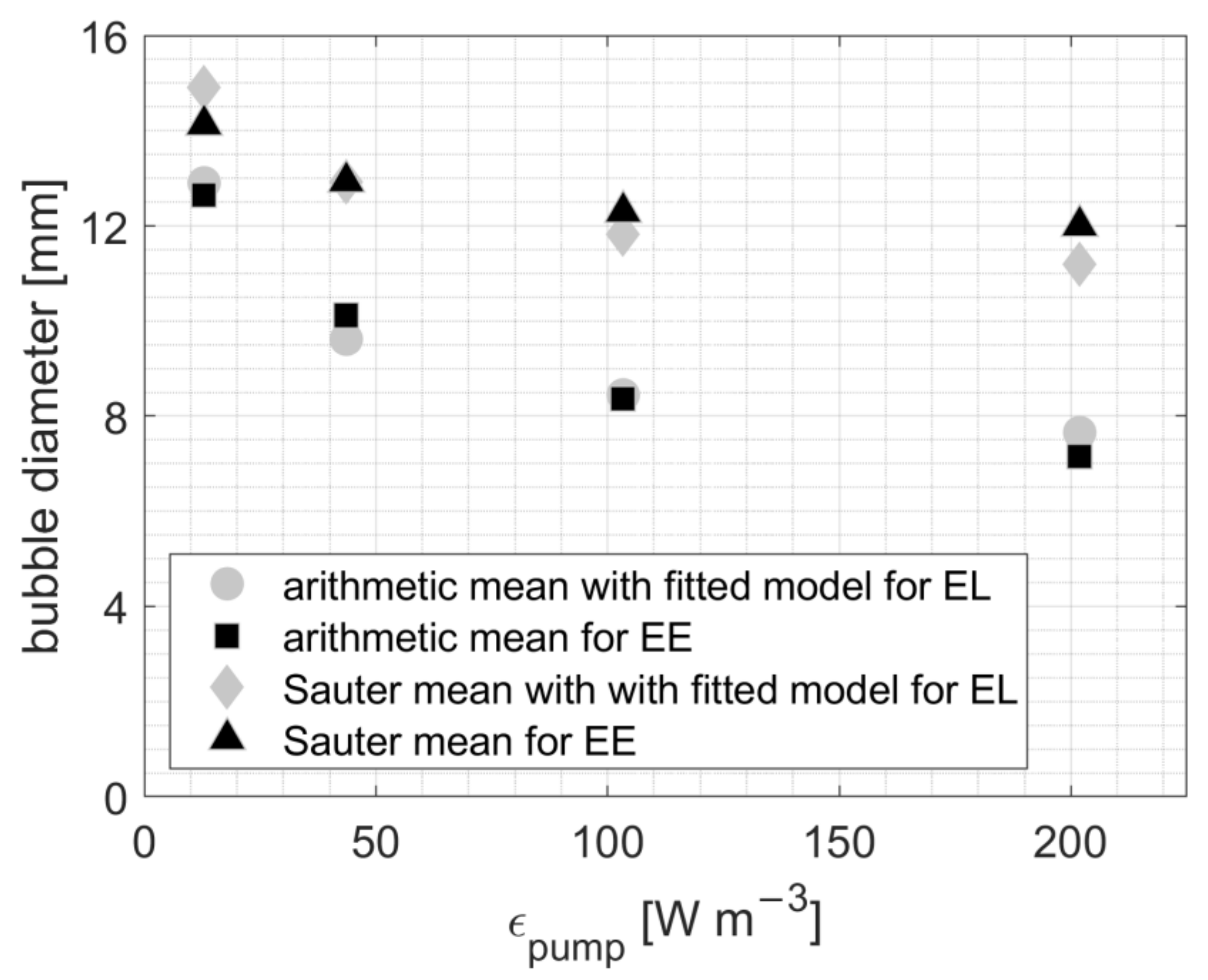
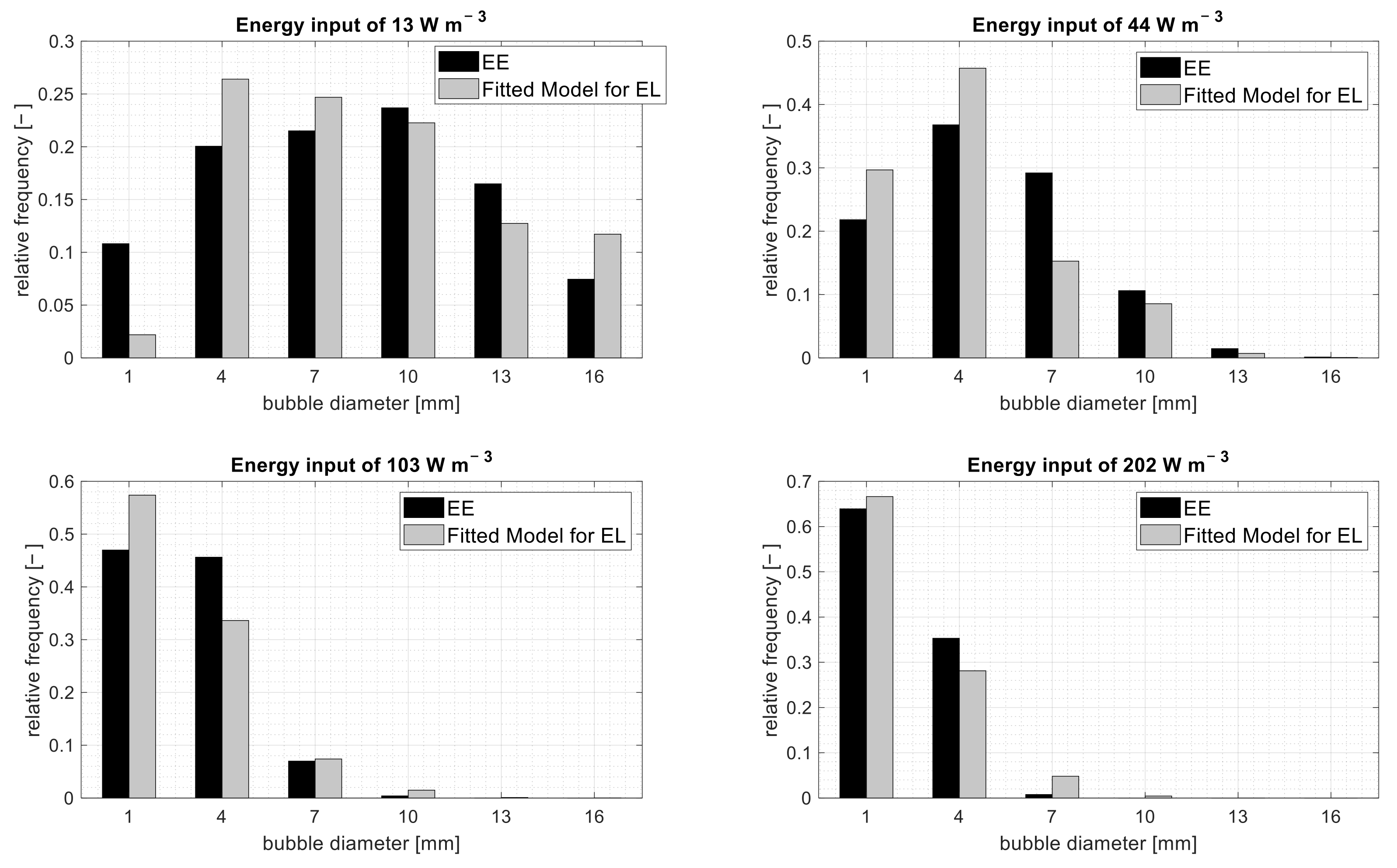
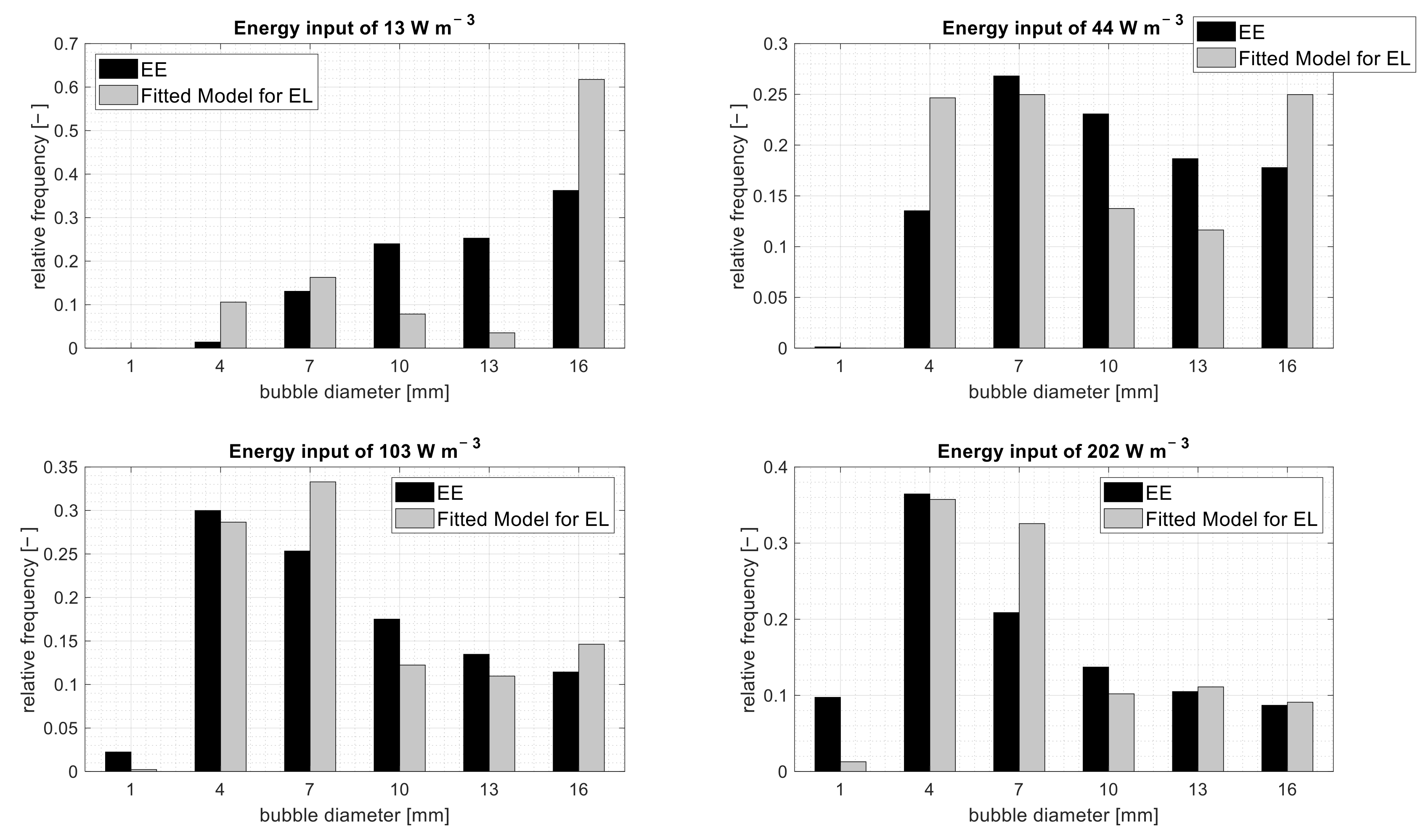
3.4. Comparison of Bubble Size Distribution between the Euler-Euler and Euler-Lagrange Approaches

The black bars in Figure 11 and Figure 12 show the resulting BSD for the Luo et al. [4] and Lehr et al. [1] models, respectively, simulated in the EE framework for different ε_pump values. The gray bars represent the results of the new model simulated in EL. The new models are able to accurately capture partial population breakage. In the case of the Lehr et al. [1] model, the portion of bubbles that undergo breakage is smaller compared to the Luo et al. model, as seen in Figure 11 and Figure 12. This effect could be maintained by using the individual levels of We_crit. The Luo et al. model predominantly generates bubbles around 1 mm in diameter due to the U-shaped DSD used, while the M-shaped DSD of the Lehr et al. model mainly produces bubbles of classes 4 and 7 mm. At ε_pump of 13 W m⁻³, a fraction of bubbles kept the initial diameter of 16 mm in the Luo et al. model, as seen in Figure 11. With an energy input of 44 W m⁻³, no bubbles are left, showing an initial diameter of 16 mm. In both simulations, bubbles with a dominant diameter of approximately 4 mm are predicted. After the energy input was increased from 103 to 202 W m⁻³, distributions changed only slightly. Increasingly, more energy is needed to cause further breakage events. Notably, the specification of discrete bins prevents the occurrence of bubbles smaller than 1 mm in the EE approach. Although this theoretical barrier does not exist for EL, bubble breakage also ends at 1 mm because the energy demand for further breakage becomes too large. In the case of the model of Lehr et al., the portion of bubbles that undergo a breakage is smaller compared to the model of Luo et al., as seen in Figure 11 and Figure 12. The fraction of bubbles that have not broken once is almost two times higher in the case of the EE approach. The DSD compensates for this effect by forming smaller bubbles, resulting in a similar Sauter diameter. The influence of the M-shape can be seen at ${\epsilon }_{pump}$ of 44 W m⁻³, since very small bubbles around the size of 1 mm are not formed at all. As the energy input increases to 103 and 202 W m⁻³, the increase in the bubble breakage rate is minor compared to ${\epsilon }_{pump}$ values of 13 and 44 W m⁻³.

It is highlighted that the complex implementation of the original DSDs in EL was the most crucial factor in reproducing EE framework results optimally in terms of bubble breakage.

4. Conclusions

A new bubble breakage description for an EL approach was formulated, consisting of a critical We_crit number, a DSD and the minimum time between two consecutive bubble breakages. Two of the most widely used bubble breakage models have been successfully adapted to the new model description using EE solutions in Ansys Fluent as a template. The presented BSD was consistent with respect to both the Sauter diameter and arithmetic diameter. Furthermore, it reproduced the distribution shape of the bubbles well. The models were validated for a wide range of bubble diameters and a broad turbulence spectrum as encountered in high-volume multiphase reactors. The breakage models have no unknown parameters since all constants were determined in the original version. As such, they are applicable to both EL simulation and the higher sophisticated LES turbulence model. Given the rising importance of LES simulation, the framework of this study may enable the proper consideration of bubble breakage events in LES, which is a prerequisite for multiphase simulations in bioreactors. We_crit represents an additional degree of freedom that acts as a fitting parameter and is adjustable to a wide range of datasets. Therefore, experimental datasets may well serve as input for realistic bubble breakage predictions in the LES context.

References

1. Lehr, F.; Mewes, D.; Millies, M. Bubble size distributions and flow fields in bubble columns. AIChE J. 2002, 42, 1225–1233. [Google Scholar] [CrossRef]
2. Laakkonen, M.; Moilanen, P.; Alopaeus, V.; Aittamaa, J. Modelling local bubble size distributions in agitated vessels. Chem. Eng. Sci. 2007, 62, 721–740. [Google Scholar] [CrossRef]
3. Zhang, H.; Yang, G.; Sayyar, A.; Wang, T. An improved bubble breakup model in turbulent flow. Chem. Eng. J. 2020, 386, 121484. [Google Scholar] [CrossRef]
4. Luo, H.; Svendsen, H.F. Theoretical model for drop and bubble breakup in turbulent dispersions. AIChE J. 1996, 42, 1225–1233. [Google Scholar] [CrossRef]
5. Siebler, F.; Lapin, A.; Hermann, M.; Takors, R. The impact of CO gradients on C. ljungdahlii in a 125 m3 bubble column: Mass transfer, circulation time and lifeline analysis. Chem. Eng. Sci. 2019, 207, 410–423. [Google Scholar] [CrossRef]
6. Huang, Z.; McClure, D.D.; Barton, G.W.; Fletcher, D.F.; Kavanagh, J.M. Assessment of the impact of bubble size modelling in CFD simulations of alternative bubble column configurations operating in the heterogeneous regime. Chem. Eng. Sci. 2018, 186, 88–101. [Google Scholar] [CrossRef]
7. Guan, X.; Xu, Q.; Yang, N.; Nigam, K.D. Hydrodynamics in bubble columns with helically-finned tube Internals: Experiments and CFD-PBM simulation. Chem. Eng. Sci. 2021, 240, 116674. [Google Scholar] [CrossRef]
8. Yan, P.; Jin, H.; Gao, X.; He, G.; Guo, X.; Ma, L.; Yang, S.; Zhang, R. Numerical analysis of bubble characteristics in a pressurized bubble column using CFD coupled with a population balance model. Chem. Eng. Sci. 2021, 234, 116427. [Google Scholar] [CrossRef]
9. Shao, P.; Liu, S.; Miao, X. CFD-PBM simulation of bubble coalescence and breakup in top blown-rotary agitated reactor. J. Iron Steel Res. Int. 2022, 29, 223–236. [Google Scholar] [CrossRef]
10. Zhou, X.; Ma, Y.; Liu, M.; Zhang, Y. CFD-PBM simulations on hydrodynamics and gas-liquid mass transfer in a gas-liquid-solid circulating fluidized bed. Powder Technol. 2020, 362, 57–74. [Google Scholar] [CrossRef]
11. Shu, S.; Zhang, J.; Yang, N. GPU-accelerated transient lattice Boltzmann simulation of bubble column reactors. Chem. Eng. Sci. 2020, 214, 115436. [Google Scholar] [CrossRef]
12. Farsani, H.Y.; Wutz, J.; DeVincentis, B.; Thomas, J.A.; Motevalian, S.P. Modeling mass transfer in stirred microbioreactors. Chem. Eng. Sci. 2022, 248, 117146. [Google Scholar] [CrossRef]
13. Kuschel, M.; Fitschen, J.; Hoffmann, M.; von Kameke, A.; Schlüter, M.; Wucherpfennig, T. Validation of Novel Lattice Boltzmann Large Eddy Simulations (LB LES) for Equipment Characterization in Biopharma. Processes 2021, 9, 950. [Google Scholar] [CrossRef]
14. Gaugler, L.; Mast, Y.; Fitschen, J.; Hofmann, S.; Schlüter, M.; Takors, R. Scaling-down biopharmaceutical production processes via a single multi-compartment bioreactor (SMCB). Eng. Life Sci. 2023, 23, e2100161. [Google Scholar] [CrossRef] [PubMed]
15. Hoppe, F.; Breuer, M. A deterministic breakup model for Euler-Lagrange simulations of turbulent microbubble-laden flows. Int. J. Multiph. Flow 2020, 123, 103119. [Google Scholar] [CrossRef]
16. Jain, D.; Kuipers, J.; Deen, N.G. Numerical study of coalescence and breakup in a bubble column using a hybrid volume of fluid and discrete bubble model approach. Chem. Eng. Sci. 2014, 119, 134–146. [Google Scholar] [CrossRef]
17. Lau, Y.M.; Bai, W.; Deen, N.G.; Kuipers, J. Numerical study of bubble break-up in bubbly flows using a deterministic Euler-Lagrange framework. Chem. Eng. Sci. 2014, 108, 9–22. [Google Scholar] [CrossRef]
18. Sungkorn, R.; Derksen, J.J.; Khinast, J.G. Euler-Lagrange modeling of a gas-liquid stirred reactor with consideration of bubble breakage and coalescence. AIChE J. 2012, 58, 1356–1370. [Google Scholar] [CrossRef]
19. Afra, B.; Karimnejad, S.; Amiri Delouei, A.; Tarokh, A. Flow control of two tandem cylinders by a highly flexible filament: Lattice spring IB-LBM. Ocean Eng. 2022, 250, 111025. [Google Scholar] [CrossRef]
20. Afra, B.; Amiri Delouei, A.; Mostafavi, M.; Tarokh, A. Fluid-structure interaction for the flexible filament’s propulsion hanging in the free stream. J. Mol. Liq. 2021, 323, 114941. [Google Scholar] [CrossRef]
21. Deen, N.G.; Solberg, T.; Hjertager, B.H. Large eddy simulation of the Gas–Liquid flow in a square cross-sectioned bubble column. Chem. Eng. Sci. 2001, 56, 6341–6349. [Google Scholar] [CrossRef]
22. Thomas, J.A.; Liu, X.; DeVincentis, B.; Hua, H.; Yao, G.; Borys, M.C.; Aron, K.; Pendse, G. A mechanistic approach for predicting mass transfer in bioreactors. Chem. Eng. Sci. 2021, 237, 116538. [Google Scholar] [CrossRef]
23. Hanspal, N.; DeVincentis, B.; Thomas, J.A. Modeling multiphase fluid flow, mass transfer, and chemical reactions in bioreactors using large-eddy simulation. Eng. Life Sci. 2023, 23, e2200020. [Google Scholar] [CrossRef] [PubMed]
24. Maly, M.; Schaper, S.; Kuwertz, R.; Hoffmann, M.; Heck, J.; Schlüter, M. Scale-Up Strategies of Jet Loop Reactors for the Intensification of Mass Transfer Limited Reactions. Processes 2022, 10, 1531. [Google Scholar] [CrossRef]
25. Tomiyama, A.; Kataoka, I.; Zun, I.; Sakaguchi, T. Drag Coefficients of Single Bubbles under Normal and Micro Gravity Conditions. JSME Int. J. Ser. B 1998, 41, 472–479. [Google Scholar] [CrossRef] [Green Version]
26. Krüger, T.; Kusumaatmaja, H.; Kuzmin, A.; Shardt, O.; Silva, G.; Viggen, E.M. The Lattice Boltzmann Method: Principles and Practice; Springer International Publishing: Cham, Switzerland, 2017; ISBN 3319446479. [Google Scholar]
27. Bhatnagar, P.L.; Gross, E.P.; Krook, M. A Model for Collision Processes in Gases. I. Small Amplitude Processes in Charged and Neutral One-Component Systems. Phys. Rev. 1954, 94, 511–525. [Google Scholar] [CrossRef]
28. Saffman, P.G. The lift on a small sphere in a slow shear flow. J. Fluid Mech. 1965, 22, 385–400. [Google Scholar] [CrossRef] [Green Version]
29. Khan, Z.; Bhusare, V.H.; Joshi, J.B. Comparison of turbulence models for bubble column reactors. Chem. Eng. Sci. 2017, 164, 34–52. [Google Scholar] [CrossRef]
30. Khan, Z.; Joshi, J.B. Comparison of k–ε, RSM and LES models for the prediction of flow pattern in jet loop reactor. Chem. Eng. Sci. 2015, 127, 323–333. [Google Scholar] [CrossRef]
31. Joshi, J.B.; Nere, N.K.; Rane, C.V.; Murthy, B.N.; Mathpati, C.S.; Patwardhan, A.W.; Ranade, V.V. CFD simulation of stirred tanks: Comparison of turbulence models. Part I: Radial flow impellers. Can. J. Chem. Eng. 2011, 89, 23–82. [Google Scholar] [CrossRef]
32. Smagorinsky, J. General Circulation Experiments With The Primitive Equations: I. The Basic Experiment. Mon. Weather Rev. 1963, 91, 99–164. [Google Scholar] [CrossRef]
33. Evrard, F.; Denner, F.; van Wachem, B. Quantifying the errors of the particle-source-in-cell Euler-Lagrange method. Int. J. Multiph. Flow 2021, 135, 103535. [Google Scholar] [CrossRef]
34. Liao, Y.; Lucas, D. A literature review of theoretical models for drop and bubble breakup in turbulent dispersions. Chem. Eng. Sci. 2009, 64, 3389–3406. [Google Scholar] [CrossRef]
35. Hinze, J.O. Turbulence, 2nd ed.; reissued; McGraw-Hill: New York, NY, USA, 1975; ISBN 0070290377. [Google Scholar]
36. Kolmogorov, A.N. On the breakage of drops in a turbulent flow. Dokl. Akad. Navk. SSSR 1949, 66, 825–828. [Google Scholar]
37. Kuboi, R.; Komasawa, I.; Otake, T. Behavior Of Dispersed Particles In Turbulent Liquid Flow. J. Chem. Eng. Jpn./JCEJ 1972, 5, 349–355. [Google Scholar] [CrossRef] [Green Version]
38. Hesketh, R.P.; Etchells, A.W.; Russell, T.W.F. Experimental observations of bubble breakage in turbulent flow. Ind. Eng. Chem. Res. 1991, 30, 835–841. [Google Scholar] [CrossRef]
39. Coulaloglou, C.A.; Tavlarides, L.L. Description of interaction processes in agitated liquid-liquid dispersions. Chem. Eng. Sci. 1977, 32, 1289–1297. [Google Scholar] [CrossRef]
40. Shuai, Y.; Wang, X.; Huang, Z.; Sun, J.; Yang, Y.; Liao, Z.; Wang, J.; Yang, Y. Experimental measurement of bubble breakup in a jet bubbling reactor. AIChE J. 2021, 67, e17062. [Google Scholar] [CrossRef]
41. Solsvik, J.; Jakobsen, H.A. Single Air Bubble Breakup Experiments in Stirred Water Tank. Int. J. Chem. React. Eng. 2015, 13, 477–491. [Google Scholar] [CrossRef]
42. Andersson, R.; Andersson, B. On the breakup of fluid particles in turbulent flows. AIChE J. 2006, 52, 2020–2030. [Google Scholar] [CrossRef]
43. Martinez-Bazan, C.; Montañés, J.L.; Lasheras, J.C. On the breakup of an air bubble injected into a fully developed turbulent flow. Part 1. Breakup frequency. J. Fluid Mech. 1999, 401, 157–182. [Google Scholar] [CrossRef] [Green Version]
44. Wilkinson, P.M. Physical Aspects and Scale-Up of High Pressure Bubble Columns. Ph.D. Thesis, Rijksuniversiteit Groningen, Groningen, The Netherlands, 1991. [Google Scholar]
45. Wang, T.; Wang, J.; Jin, Y. Population Balance Model for Gas−Liquid Flows: Influence of Bubble Coalescence and Breakup Models. Ind. Eng. Chem. Res. 2005, 44, 7540–7549. [Google Scholar] [CrossRef]
46. Guo, K.; Wang, T.; Liu, Y.; Wang, J. CFD-PBM simulations of a bubble column with different liquid properties. Chem. Eng. J. 2017, 329, 116–127. [Google Scholar] [CrossRef]
47. Battistella, A.; Aelen, S.; Roghair, I.; van Sint Annaland, M. Euler-Lagrange Modeling of Bubbles Formation in Supersaturated Water. ChemEngineering 2018, 2, 39. [Google Scholar] [CrossRef] [Green Version]
48. Galinat, S.; Risso, F.; Masbernat, O.; Guiraud, P. Dynamics of drop breakup in inhomogeneous turbulence at various volume fractions. J. Fluid Mech. 2007, 578, 85–94. [Google Scholar] [CrossRef]
49. Prince, M.J.; Blanch, H.W. Bubble coalescence and break-up in air-sparged bubble columns. AIChE J. 1990, 36, 1485–1499. [Google Scholar] [CrossRef]
Figure 1. Mesh for bubble column simulation in Ansys Fluent. (a): View from the top (b): Section view from the side.
Processes 11 01018 g001
Figure 2. Mesh independence study with 3 different mesh densities. The turbulent dissipation rate on a vertical line in the center of the column is compared. (a): Ansys Fluent simulation (b): M-Star simulation.
Processes 11 01018 g002
Figure 3. Flow field as contour plot shown as a section plane, where turbulent dissipation rate is depicted. Simulation of bubble column in Ansys Fluent. (a): Ansys Fluent simulation (b): M-Star simulation.
Processes 11 01018 g003
Figure 4. Prediction of daughter size distributions using the approach of Luo et al. for different parent bubble sizes with the set value ε = 0.08 W m−3.
Processes 11 01018 g004
Figure 5. Prediction of daughter size distributions using the approach of Lehr et al. for different parent bubble sizes with the set value ε = 0.1 W m−3.
Processes 11 01018 g005
Figure 6. Overview of fitting parameters for the EL breakage model. The function, as well as the method for the determination of the parameters, is illustrated. The left column depicts the bubble breakage implementation in EE and the right column shows how the implementation is transferred into an EL implementation. (Top left): Different bubble sizes exist in a PBM solely as distribution quantities that shift into smaller classes in case of a breakage. (Top right): A breakage of an individual bubble is executed only if the breakage criterion in the form of W e c r i t is exceeded. (Center left): The shape of the DSD changes three-dimensionally with varying bubble diameters and turbulent dissipation energy. (Center right): The shape of the DSD changes solely with varying bubble diameter and the influence of the turbulent dissipation energy is replaced by a constant. (Bottom left): The integro-differential equation of the PBM calculates bubble breakage events per unit of time. (Bottom right): After an executed bubble breakage, a subsequent division can take place at the earliest after the time t b r e a k .
Processes 11 01018 g006
Figure 7. The summed deviation of the Sauter mean bubble diameter for different critical We numbers of the fitted model for Luo et al. recreation.
Processes 11 01018 g007
Figure 8. The summed deviation of the Sauter mean bubble diameter for different critical We numbers of the fitted model for Lehr et al. recreation.
Processes 11 01018 g008
Figure 9. Arithmetic diameter and Sauter diameter of the bubble breakage model given by Luo et al. The solution is compared with the EE approach and the fitted model in EL. Shown for pump volume flow 13, 44, 103 and 202 W m−3.
Processes 11 01018 g009
Figure 10. Arithmetic diameter and Sauter diameter of the bubble breakage model given by Lehr et al. The solution is compared with the EE approach and the fitted model in EL. Shown for pump volume flow 13, 44, 103 and 202 W m−3.
Processes 11 01018 g010
Figure 11. Comparison of the resulting bubble size distribution created with the Luo et al. [4] model in the EE approach (black) and the fitted model for EL (gray). Shown for energy input of 13, 44, 103 and 202 W m−3.
Processes 11 01018 g011
Figure 12. Comparison of the resulting bubble size distribution created with the Lehr et al. [1] model in the EE approach (black) and the fitted model for EL (gray). Shown for energy input of 13, 44, 103 and 202 W m−3.
Processes 11 01018 g012