Optimal Control of Hybrid Photovoltaic/Thermal Water System in Solar Panels Using the Linear Parameter Varying Approach

Abstract

During photovoltaic (PV) conversion in solar panels, a part of the solar radiation is not converted to electricity by the cells, producing heat that could increase their temperature. This increase in temperature deteriorates the performance of the PV panel. In this paper, a hybrid PV/thermal (PV/T) water system is proposed to mitigate this problem. This system combines a PV panel and a thermal collector. In this paper, we focused on the modeling and control of this hybrid system in the linear parameter varying (LPV) framework. An optimal linear quadratic regulator (LQR) is proposed to control the PV cell temperature around an optimal value that maximises electricity generation. Since the system model is nonlinear, an optimal LQR gain-scheduling state-feedback control approach based on an LPV representation of the nonlinear model is designed using the Linear Matrix Inequality (LMI) method. The goal is to obtain the maximum electrical power for each solar panel. Since a reduced number of sensors is available, an LPV Kalman filter is also proposed to estimate the system states required by the state-feedback controller. The obtained results in a laboratory setup in simulation are used to assess the proposed approach, showing promise in terms of control performance of the PV/T system.

1. Introduction

Presently, electrical energy is necessary for almost all human activities around the world. Due to large population growth, the demand for electricity has increased tremendously in recent decades. In many countries, electricity generation still depends mainly on fossil fuel technology that requires huge financial resources in addition to contributing to climate change. With the aim of reducing the use of fossil fuel technology and avoiding environmental damage [1,2,3], the world is moving towards the production of electricity by using renewable energies because of their advantages, such as pollution and greenhouse gas emissions reduction and their wide availability around the world [4,5]. For this reason, renewable energies are increasingly attracting the interest of many energy utilities. This is the reason why renewable energies are becoming crucial and will play an important role in the economic development of all countries in the near future [6,7,8].

In order to limit global warming and reduce environmental contamination, several countries agreed to limit emissions according to the Paris convention signed at a conference on climate change held in the United States in 2015 [9,10]. Moreover, many countries are moving towards increasing the consumption of renewable energy as a solution to reduce CO${}_2$ emissions and the production costs of using expensive fossil fuels.

Researchers and country leaders are currently focusing on harnessing green energies such as wind energy, ocean energy and solar energy [11].

Solar energy is one of the most developed clean and renewable energies today; its advantages are pollution reduction and protection of the environment. The use of this type of energy is also less costly compared to other types of energy.

Like other types of energy generation technologies, photovoltaic (PV) solar energy also has some disadvantages because solar systems are generally installed outside and will be directly exposed to climatic factors such as high temperature, wind and shading. All these factors cause a decrease in their efficiency. For this reason, several works are dedicated to studying and developing PV technology to obtain better performance. After several tests on PV systems, researchers and photovoltaic industries found that an increase in temperature could lead to a performance reduction in PV cells [12]. To mitigate this problem, many efforts have been made in order to increase their efficiency and subsequently reduce the cost of their maintenance.

Given the importance of this energy generation technology and its simplicity of use, many researchers in the PV domain are interested in improving the performance of solar panels in order to extract the maximum electrical power, e.g., by modifying the structure and design of solar panels [13]. The application of feedback control as suggested in [14] allows the design of a controller based on the prediction of DC voltage that allows the three-phase inverter to follow the maximum power despite the disturbances of climatic conditions and the variable loads. There are also other works aiming at regulating the PV cells’ temperature in order to improve the performance of the panels, such as, e.g., [15], where the researchers use a phase change material for cooling the PV panels under Malaysian weather conditions. The result shows that the surface temperature of the module is reduced by 10 ${}^{°}$C, which remains constant for a period of 4 to 6 h. In [16], two different methods were used to regulate the PV cell temperature without the interference of any other external mechanism. The first one is based on using argon gas within the concentrator element, and the second one is based on the incorporation of polymer-dispersed liquid crystal films (PDLC) on top of the module. In both cases, the power was improved by 37 mW–47 mW while temperature was reduced by 10 ${}^{°}$C and 4 ${}^{°}$C for the argon gas-filled module and PDLC integrated module, respectively. In [17], the cooling system uses a simple pipe which is placed on the PV module as a spiral heat exchanger in order to provide active cooling without any controller. The results show a slight decrease in the temperature of the PV module. Also, in [18], the authors of experimental and theoretical studies on the cooling of photovoltaic panels propose a solution based on the principle of evaporative cooling. The results show that the temperature of the photovoltaic panel can be reduced by 10∘ C and that the improvement in power obtained is 5%. A PID controller allows the adjustment of a cooling mechanism such as a fan or heat sink to regulate the temperature of the solar panel. There are other works dedicated to the development of solar cell technologies and the mounting structures of PV modules, such as, e.g., [19,20,21,22], aiming at extracting more energy.

Due to their importance and advantages, hybrid PV/T systems have gained great attention from manufacturers in recent years. A PV/T system can produce two types of energy, electrical energy (electrical power $P_e$) and thermal energy (thermal power $Q_t$). Given the reality of global warming, it is likely that cooling and heating needs in buildings will increase. In this regard, the use of a hybrid PV/T system appears to be a very suitable solution as these systems can supply both heating and cooling depending on the specific needs of the user [22,23,24,25]. While this type of hybrid system has advantages, they can also have disadvantages related to the production and installation costs of PV-T collectors, which are still high. Moreover, certain technological improvements are necessary, including research and development of new materials, system stability improvements and the design of a supporting energy storage system [26]. There are two types of PV/T hybrid systems. The first one is a hybrid PV/T air system which is able to produce electricity and heat, where the cooling technique of the PV module is made by the circulation of air in the collector. The second one is a hybrid PV/T water system able to produce electricity and hot water, which is the subject of this paper. These systems can be covered or uncovered using different types of PV cells (e.g., monocrystalline silicon cells, polycrystalline silicon cells, amorphous silicon cells or thin-film cells, among others).

Usually, a classic PV model absorbs between 80 and 90% of solar radiation but only 10 to 20% has been converted into electricity and the rest is transformed into heat which can be a damaging factor for PV cells [27]. The PV/T system can remedy this problem and improve the efficiency of the PV cell by producing at the same time heat or hot water for users [28].

In recent years, several researchers have been interested in the control of PV/T hybrid water systems in order to improve performance [29,30,31]. A model predictive control is used to optimally control the operation of an HVAC system based on a hybrid PV/T system [32]. A controller based on an Artificial Neural Network (ANN) is proposed to improve performance and track optimum electrical and thermal power in [33], and in [34], where a PV/T ANN-based control algorithm was applied to detect the optimum electrical and thermal power operating point (OPOP). OPOP makes it possible to find the optimal water flow rate of a PV/T system for a given ambient temperature and solar irradiation, facilitating the extraction of maximum energy. The results showed that the application of an ANN, with one hidden layer for the thermal and electrical modeling of the PVT collector, makes it possible to improve performance using training data obtained from real experiments.

This paper investigates how to increase the performance of a hybrid PV/T water system by controlling the temperature of PV cells. The research work presented has a twofold objective: on the one hand, to implement and design an optimal LQR controller to decrease the PV cell temperature caused by the increase in ambient temperature and irradiation around an optimal value equal to 25 ${}^{°}$C in order to extract the maximum energy, and on the other hand, to prove the effectiveness of this controller against external disturbances. Since the system model is nonlinear, an optimal LQR gain-scheduling state-feedback control approach based on an LPV representation of the nonlinear model is designed using the Linear Matrix Inequality (LMI) method. The goal is to obtain the maximum electrical power for each solar panel. Since a reduced number of temperature sensors are available, an LPV Kalman filter is also proposed to estimate the system states required for the state-feedback controller. The obtained results in simulation using a pilot-prototype installation have allowed the assessment of the proposed control method showing an improvement in electricity generation. Furthermore, the proposed approach allows us to obtain an optimal performance compared to other types of control presented in the literature [35,36,37].

The structure of the remainder of the paper is as follows: Section 2 describes the PV/T hybrid system used as case study. Section 3 deals with the modeling of a PV/T hybrid system using physical principles. Section 4 develops a control-oriented model in the LPV framework using the nonlinear embedding approach. Section 5 presents an optimal LQR gain-scheduling state-feedback control approach based on an polytopic representation of the LPV model. In Section 6, a state estimator based on an LPV Kalman filter is designed to estimate all the unknown system states. Finally, the main conclusions and remarks are drawn in Section 7.

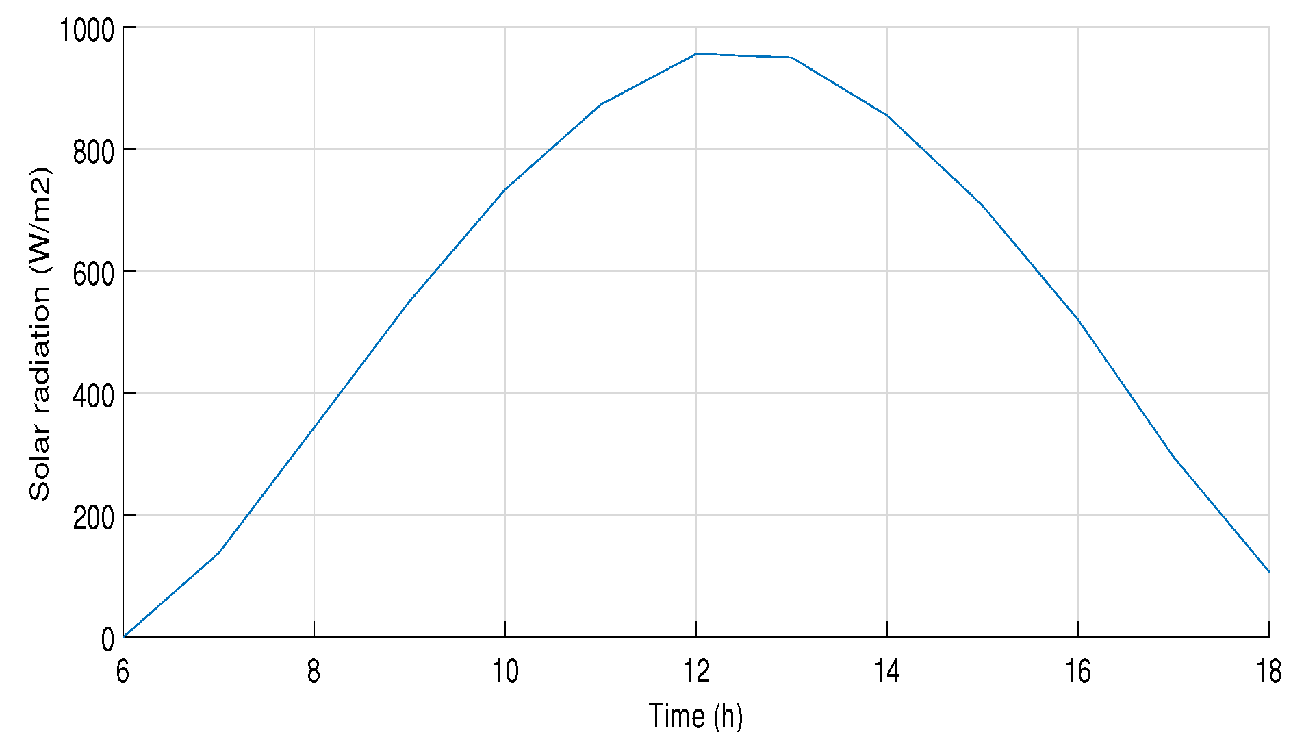
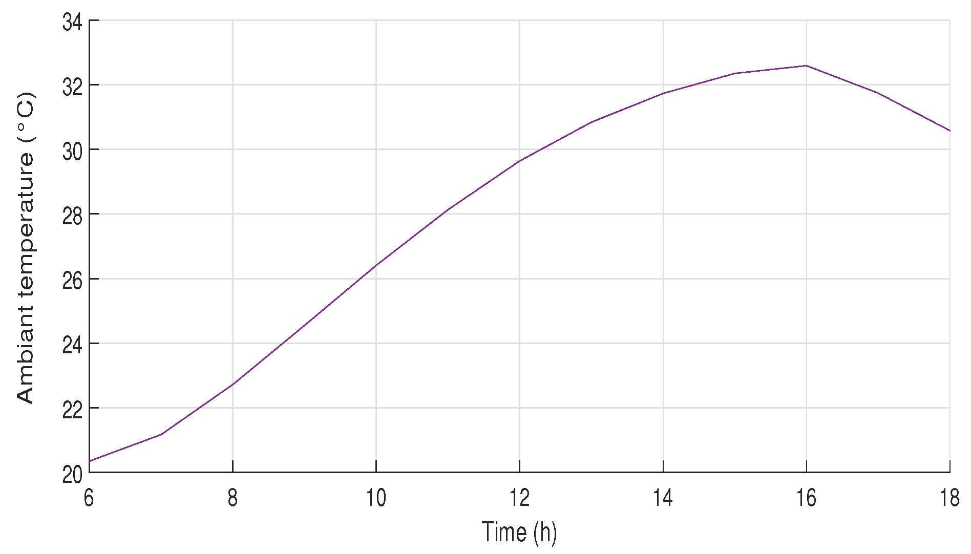
2. Case Study Description

Figure 1a,b show the hybrid PV/T water system (VOLTHER PowerTherm) and its schematic diagram installed at the Research and Technology Center of Energy (CRTEn) located in the northern part of Tunisia, which was used in this paper as a case study. The considered PV/T hybrid system refrigerated with water combines two different subsystems: a photovoltaic panel (PV) and a thermal collector (T) to form the PV/T system. This system can be installed in a photovoltaic field connected to the utility grid via a smart power inverter without any effect on its operation [38]. As discussed in the introduction, the purpose of this hybrid system is to reduce the PV cell temperature ($T_c$) and subsequently increase the produced electrical power.

The configuration of the system is composed of a hybrid PV/T system, a water tank, a pump that allows the circulation and variation of the water flow rate in the absorber installed under the PV cells and an I-V 400W device to measure the current, the temperature and the evolution of the electrical and thermal power in real conditions of solar radiation and ambient temperature [39].

During the operation of this system, when the ambient temperature and the solar radiation increases, the temperature of the PV cell ($T_c$) gradually increases and directly affects the PV performance. To solve this problem, the PV cell temperature must be decreased. As discussed in the introduction, results presented in the literature have shown that water cooling, although it could be expensive, is the most effective cooling technique. The circulation of water in the absorber is carried out by the circulation pump which allows reduction of the temperature of the PV cell. The cooling method for PV cells through the circulation of water in the absorber has limitations, as it only marginally reduces the temperature of the PV cell. This was substantiated through an experimental test conducted on the actual prototype located in the CRTEn laboratory mentioned in [40]. Despite employing water as a cooling fluid, the temperature of the PV cells persistently remains elevated. Consequently, the implementation of an optimal controller emerges as a suitable solution.

At the output of the absorber, water is recovered at a high temperature and the power delivered by the PV panel will be stored in the batteries if this system is installed in isolated sites, or injected directly into the utility grid [41]. In order to increase electricity production, PV cell temperature must be controlled, taking into account the increase or decrease in the ambient temperature.

The evolution of the solar radiation G and the ambient temperature $T_a$ during a day in the CRTEn laboratory, where the system is installed, is presented in Figure 2 and Figure 3, corresponding to data collected in a real scenario.

The radiation G and the ambient temperature $T_a$ are considered disturbances. These disturbances will directly affect the performance of the photovoltaic cells, i.e., the extracted electrical power.

Figure 4 presents a conceptual representation of the hybrid PV/T water system. The considered hybrid PV/T water system (type VOLTHER PowerTherm) consists of 72 monocrystalline cells that are covered by a glass layer. Each cell is composed of three layers: a PV cell, an absorber layer in which the coolant circulates (in this paper, cold water) and a Tedlar layer for protection against humidity.

3. PV/T Water System Control-Oriented Model

As we mentioned above, the case study system is composed of two different main systems: a covered electrical system including the photovoltaic (PV) panel and a thermal system including the thermal collector (T). Following [34], the control-oriented mathematical modeling will be described in the following.

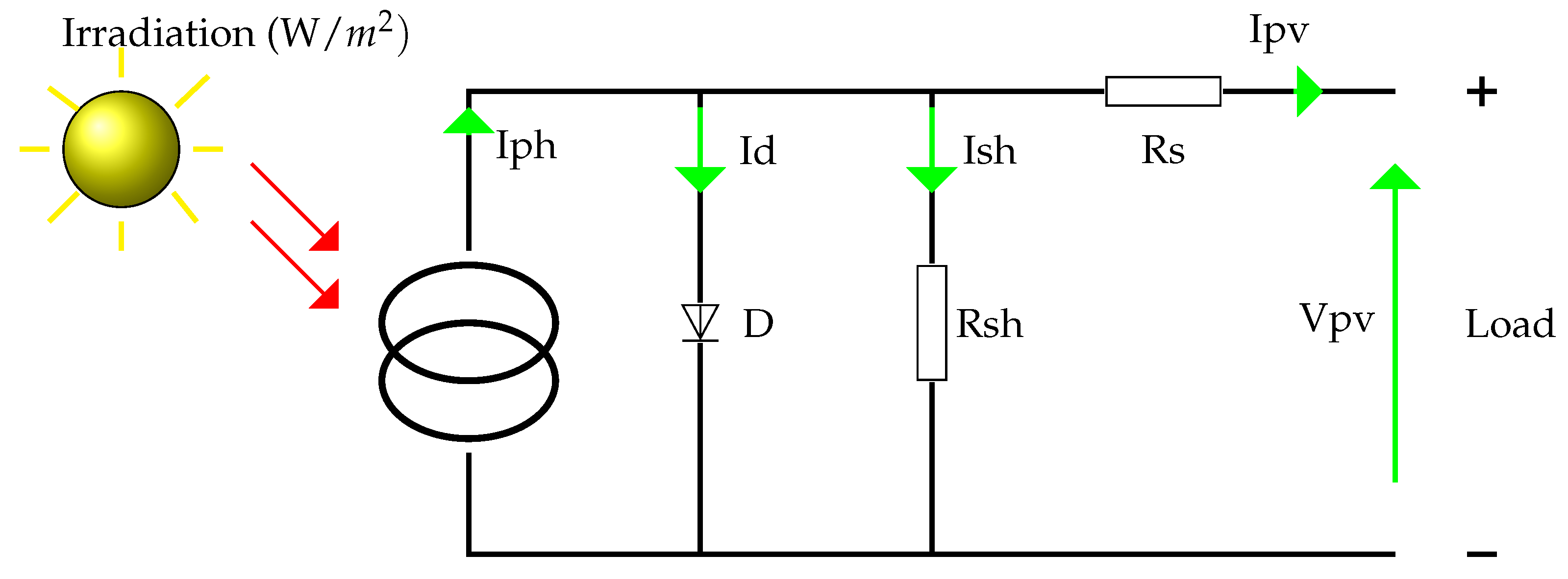
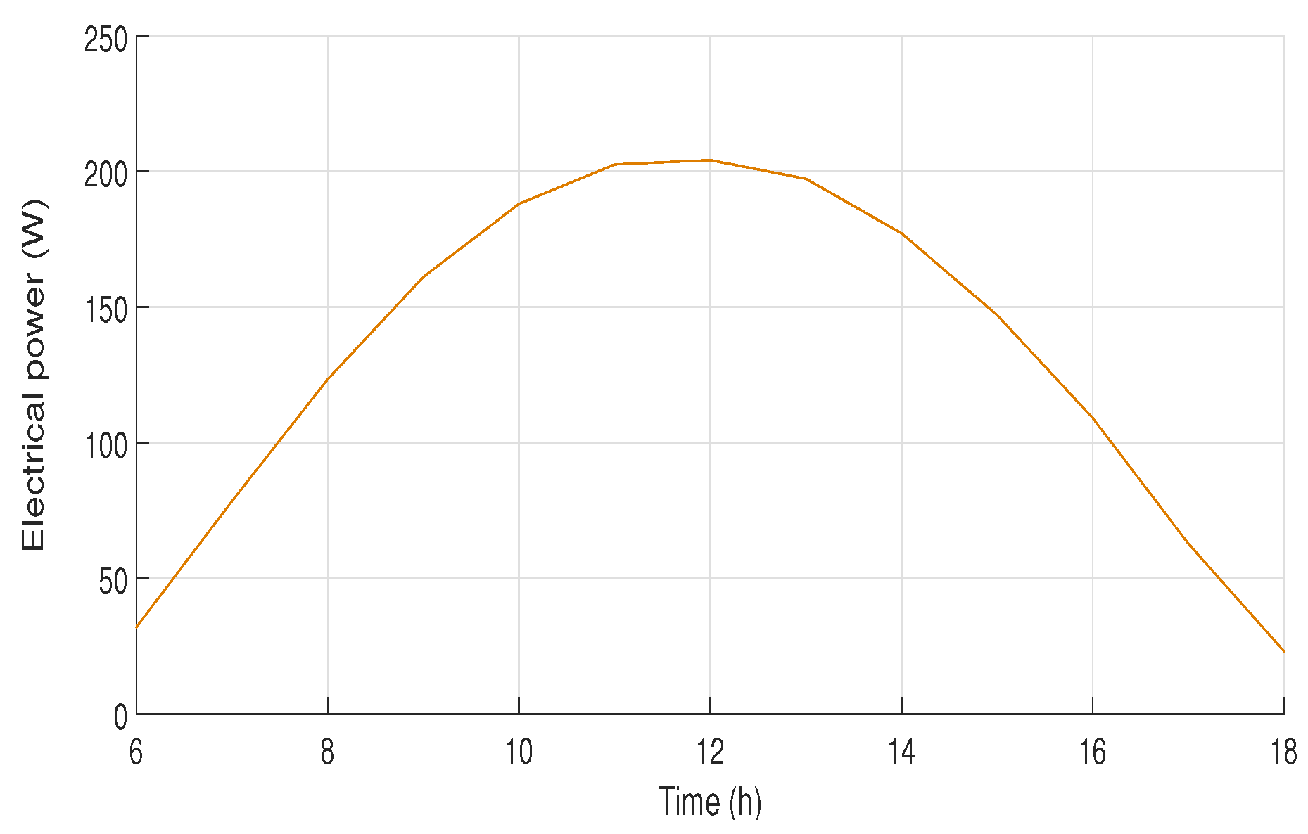
3.1. Electrical System Modeling

Figure 5 shows the model of the monocrystalline PV cell.

By exposing the PV panels to the solar radiation, the PV cell will generate electrical power that is stored in a battery or injected directly into the electrical grid.

The PV cell output current $I_{pv}$ is given by

$$I_{pv}=I_{ph}-I_d-I_{sh}$$

(1)

where $I_d$ is the current in the diode

$$\begin{array}{c}\hfill I_d=I_{rs}{e}^{q(\frac{V_{pv}+R_s{I}_{pv}}{akT{N}_s})}-1\end{array}$$

(2)

and the current $I_{sh}$ is given by

$$\begin{array}{c}\hfill I_{sh}=\frac{q(V_{pv}+R_s{I}_{pv})}{R_{sh}{R}_s}\end{array}$$

(3)

In the previous equations, $I_{pv}$, $I_{ph}$ and $I_{rs}$ are, respectively, the load current, the photoelectric current and the saturation current of the diode. $V_{pv}$ is the load voltage. $N_s$ and $N_p$ are the number of cells in series and in parallel, respectively. $R_s$, $R_{sh}$ are the series and shunt resistance, respectively. k is the Boltzmann constant equal to 1.38 $\times {10}^{-23}$ J/${}^{°}$K, q is the electron charge equal to 1.6 $·{10}^{-19}{}^{°}$C and a is the ideality factor of the diode. $I_{ph}$ is the photoelectric current given by

$$\begin{array}{c}\hfill I_{ph}=\frac{I_{ph}}{e^{q(\frac{V_{oc}}{akT{N}_s})}-1}\end{array}$$

(4)

The electrical power $P_{pv}$ of a PV cell is given by

$$\begin{array}{c}\hfill P_{pv}=V_{pv}{I}_{pv}\end{array}$$

(5)

where $V_{pv}$ represents the PV voltage.

The electrical efficiency ${\eta }_{elec}$ of the PV cell is

$$\begin{array}{c}\hfill {\eta }_{elec}=\frac{P_{pv}}{S_{pv}G}\end{array}$$

(6)

where $P_{pv}$ is total electrical power, G is the solar radiation (w/m${}^2$) and $S_{pv}$ is the PV model surface (m${}^2$).

This electrical efficiency can also be assessed as follows [42,43]

$$\begin{array}{c}\hfill {\eta }_{elec}={\eta }_{T_{ref}}[1-\beta (T_{pv}-T_{ref})]\end{array}$$

(7)

where $\beta$ is the temperature coefficient of the PV module, defined by the designer and equal to ⋍ 0.0045 ${}^{°}$K${}^{-1}$, $T_{ref}$ is the reference temperature equal to 25 ${}^{°}$C and ${\eta }_{T_{ref}}$ is the efficiency at the reference temperature.

3.2. Thermal System Modeling

The thermal modeling of the studied PV/T system is essentially based on the principle of energy conversion [13]. In order to determine the evolution of temperatures and thermal performance of each layer, the principle of energy conversion is established as

$$\begin{array}{c}\hfill M_i{C}_i\frac{d{T}_i\left(t\right)}{dt}=\sum Q_i^e\left(t\right)-\sum Q_i^s\left(t\right)\end{array}$$

(8)

where $M_i$ is the component mass, $C_i$ is the specific heat capacity of the component, $T_i$ is the component temperature, and $\sum Q_i^e$ and $\sum Q_i^s$ are, respectively, the sum of the energies received/lost by i-th layer through the heat exchanges due to conduction, convection and radiation.

The thermal modeling of the real PV/T hybrid case study system presented in Figure 4 allows us to determine the energy balance of each layer (glass cover, PV cell, absorber and fluid circulation). The mathematical model describing the evolution of the temperature of each layer in function of the water flow ($\dot{m}$), the solar radiation (G) and the ambient temperature ($T_a$) is the following [34]

• Glass layer temperature ($T_v$):

  $$\begin{array}{c}\hfill \begin{array}{c}\hfill C_v{M}_v\frac{d{T}_v\left(t\right)}{dt}={\alpha }_{v}G\left(t\right)A_v+A_v(h_{win}+h_{rva})(T_a\left(t\right)-T_v\left(t\right))+\\ \hfill A_v{h}_{rcv}(T_c\left(t\right)-T_v\left(t\right))+A_v{h}_{cv}(T_c\left(t\right)-T_v\left(t\right))\end{array}\end{array}$$

  (9)
• Cell layer temperature ($T_c$):

  $$\begin{array}{c}\hfill \begin{array}{c}\hfill C_c{M}_c\frac{d{T}_c\left(t\right)}{dt}=\left({\alpha }_{c}G{A}_c{\tau }_v(1-{\nu }_r)\right)-A_v{h}_{rcv}(T_v\left(t\right)-T_c\left(t\right))-\\ \hfill A_v{h}_{cv}(T_c\left(t\right)-T_v\left(t\right))-A_c{h}_{cp}(T_c\left(t\right)-T_p\left(t\right))\end{array}\end{array}$$

  (10)
• Absorber layer temperature ($T_p$):

  $$\begin{array}{c}\hfill \begin{array}{c}\hfill C_p{M}_p\frac{d{T}_p\left(t\right)}{dt}=(A_c{h}_{cp}(T_c\left(t\right)-T_p\left(t\right))-A_c{h}_{pa}(T_p\left(t\right)-T_a\left(t\right))-\\ \hfill A_f{h}_{fa}(T_f\left(t\right)-T_a\left(t\right))-\dot{m}{C}_f\Delta T_f\left(t\right)\end{array}\end{array}$$

  (11)
• Fluid layer temperature ($T_f$):

  $$\begin{array}{c}\hfill \begin{array}{c}\hfill C_f{M}_f\frac{d{T}_f\left(t\right)}{dt}=A_f{h}_{pf}(T_p\left(t\right)-T_f\left(t\right))\end{array}\end{array}$$

  (12)

In the previous equations, there are several heat transfer coefficients defined as follows:

-

$h_{rcv}$ is the radiation heat transfer coefficient between the glass cover and the absorber

$$h_{rcv}=\frac{\sigma (T_v^2+T_a^2)(T_v+T_a)}{(\frac{1}{{ϵ}_v}+\frac{1}{{ϵ}_c})-1}$$

(13)

-

$h_{cv}$ is the convective heat transfer coefficient between the glass cover and the PV cell

$$h_{cv}={[\frac{{\delta }_v}{k_v}+\frac{{\delta }_c}{k_c}]}^{-1}$$

(14)

-

$h_{win}$ is the convective heat transfer coefficient according to [44,45]:

$$h_{win}=2.8+3w_s$$

(15)

-

$h_{rva}$ is the radiation heat transfer coefficient between the glass cover and the environment

$$h_{rva}={ϵ}_v\sigma (T_v^2+T_a^2)(T_v+T_a)$$

(16)

The real parameters used in the simulation of the considered hybrid PV/T water system (type VOLTHER PowerTherm) available in the CRTEn laboratory are listed in

Table 1. Real parameters of PV/T system (VOLTHER PowerTherm).

Parameters	Value
Glass cover layer
Area of Glass ($A_v$)	1.64 m${}^2$
Mass of Glass ($m_v$)	7.2 kg
Specific heat capacity ($c_v$)	790 J/kg/K
Emissivity (${ϵ}_v$)	0.88
Transmissivity (${\tau }_v$)	0.95
Thickness (${\delta }_v$)	0.004 m
Absorber layer
Area of Absorber ($A_p$)	2 m${}^2$
Mass of Absorber ($m_p$)	9.03 kg
Specific heat capacity ($c_p$)	900 J/kg/K
PV cell layer
Area of PV module ($A_c$)	0.87 m${}^2$
Mass of PV module ($m_c$)	5.4 kg
Specific heat capacity ($c_c$)	860 J/kg/K
Emissivity (${ϵ}_c$)	0.93
Thickness (${\delta }_c$)	0.0003 m
Water layer
Area of fluid channel ($A_f$)	0.165 m${}^2$
Specific heat capacity ($c_f$)	4180 J/kg/K
$h_{pf}$	100
$h_{cp}$	5.7
$h_{fa}$	300

.

The previous thermal mathematical model of the system can be represented in nonlinear state-space form as follows:

$$\begin{array}{c}\dot{x}\left(t\right)=f(x\left(t\right),u\left(t\right),d\left(t\right))\hfill \\ y\left(t\right)=h\left(x\right(t),u(t\left)\right)\hfill \end{array}$$

(17)

where x = [$T_v,T_c,T_p,T_f$]${}^{⊺}$ is the state vector that represents, respectively, the temperature of each layer, u = $\dot{m}$ is the control input that corresponds to the water flow rate, d = [$G,T_a$]${}^{⊺}$ is the disturbance vector that contains the solar radiation (G) and the ambient temperature ($T_a$), and y = [$P_e,Q_t$]${}^{⊺}$ is the output vector that contains the measurements provided by the available sensors that provide the electrical power ($P_e$) and the thermal power ($Q_t$). f and g are vectorial functions that are obtained from the physical model.

4. LPV Modeling of the PV/T System

4.1. LPV Model

The thermal model (17) is nonlinear. Using the LPV approach, the nonlinearities are embedded in some varying parameters ${\theta }_{ij}$ in the function of the temperatures of each layer. The LPV model is obtained using the nonlinear embedding method proposed in [46] leading to a linear time-varying system, whose state-space representation depends on some varying parameters $\theta$

$$\begin{array}{c}\dot{x}\left(t\right)=A\left(\theta \right)x\left(t\right)+Bu\left(t\right)+B_{d}d\left(t\right)\hfill \\ y\left(t\right)=Cx\left(t\right)\hfill \end{array}$$

(18)

where the state vector $x\in {\mathbb{R}}^{n_x}$, control input $u\in {\mathbb{R}}^{n_u}$, output vector $y\in {\mathbb{R}}^{n_y}$ and disturbance vector $d\in {\mathbb{R}}^{n_d}$ are defined in the same manner as in the nonlinear model (17). $A\in {\mathbb{R}}^{n_x\times n_x}$, $B\in {\mathbb{R}}^{n_x\times n_u}$, $B_d\in {\mathbb{R}}^{n_x\times n_d}$ and $C\in {\mathbb{R}}^{n_y\times n_x}$ are the system matrices. Note that $A\left(\theta \right)$ is a matrix that contains some varying parameters ${\theta }_{ij}$ that depend on the state vector x (temperatures of the layers) and embed all the nonlinearities of the nonlinear model (17). In particular, the obtained state matrix $A\left(\theta \right)$ contains four varying parameters ${\theta }_{ij}$

$$\begin{array}{c}\hfill A\left(\theta \right)=\left[\begin{array}{cccc}{\theta }_{11}& {\theta }_{12}& a_{13}& a_{14}\\ {\theta }_{21}& {\theta }_{22}& a_{23}& a_{24}\\ a_{31}& a_{32}& a_{33}& a_{34}\\ a_{41}& a_{42}& a_{43}& a_{44}\end{array}\right]\end{array}$$

(19)

with the following expressions

$$\begin{array}{c}\hfill {\theta }_{11}=\frac{-A_v(h_{win}+h_{rva}+h_{rcv}+h_{cv})}{\left(c_v{m}_v\right)}\end{array}$$

(20)

$$\begin{array}{c}\hfill {\theta }_{12}=\frac{A_v(h_{rcv}+h_{cv})}{\left(c_v{m}_v\right)}\end{array}$$

(21)

$$\begin{array}{c}\hfill {\theta }_{21}=\frac{-A_v(h_{rcv}+h_{cv})}{\left(c_c{m}_c\right)}\end{array}$$

(22)

$$\begin{array}{c}\hfill {\theta }_{22}=\frac{-A_c{h}_{cp}-A_v{h}_{cv}+A_v{h}_{rcv}}{\left(c_c{m}_c\right)}\end{array}$$

(23)

The rest of the parameters $a_{ij}$ are constant.

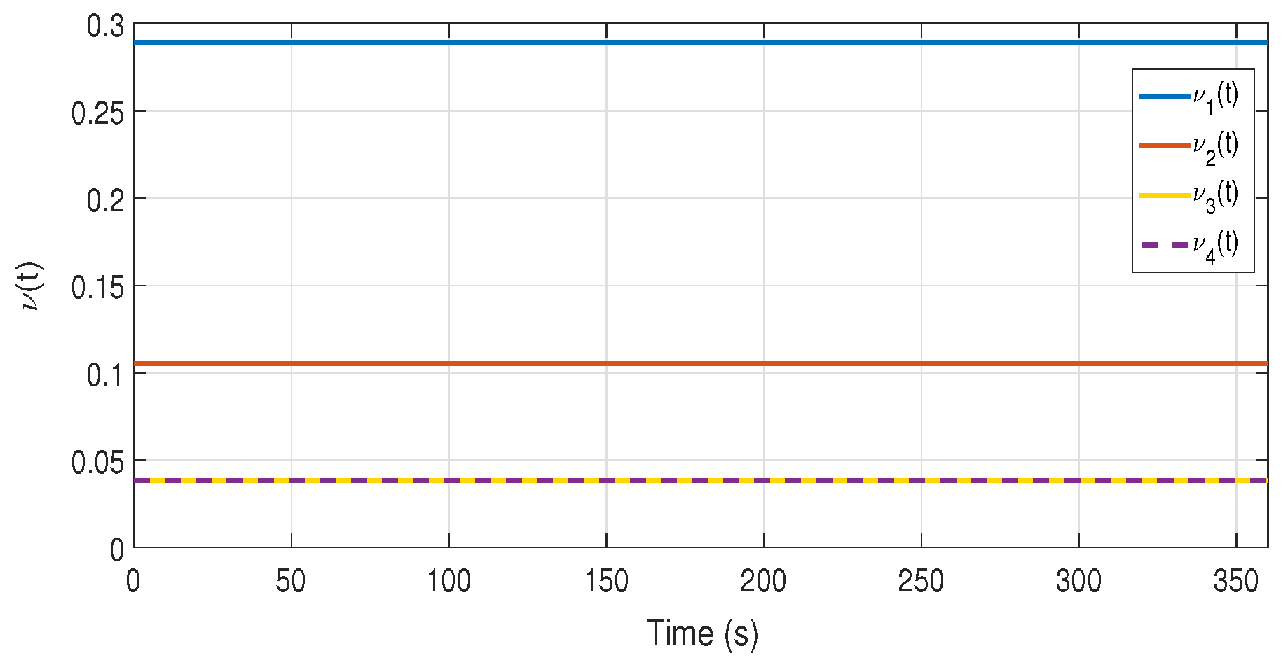
4.2. Polytopic LPV Model

To design the optimal LQR gain-scheduling controller and associated state estimator, we will transform the LPV model above in a polytopic representation using the bounding box approach [47]. Analysing the expressions of the varying parameters (20)–(23), they depend on the glass cover temperature $T_v$ and the ambient temperature $T_a$ according to (13) and (16). Using the minimum and maximum values of these two temperatures in the considered operating range, we can derive the vertex matrices $A_i$ of the polytopic representation of the matrix $A\left(\theta \right)$

$$\begin{array}{c}\hfill \begin{array}{c}\hfill \dot{x}\left(t\right)=\sum _{i=0}^N{\nu }_i\left(\theta \right)(A_{i}x\left(t\right)+B_{i}u\left(t\right))\end{array}\end{array}$$

(24)

with ${\sum }_{i=0}^N{\nu }_i\left(\theta \right)$ = 1, and 0 ≤${\nu }_i\left(\theta \right)$≤ 1, for $i=1,\cdots ,N$ with $N=2^{n_{\theta }}$ being $n_{\theta }$ the number of varying parameters.

As we have four varying parameters ${\theta }_{ij}$, we will have $N=16$ different matrices considering all the possible minimum/maximum values.

$$A_1=\left[\begin{array}{cccc}\underline{{\theta }_{11}}& \underline{{\theta }_{12}}& a_{13}& a_{14}\\ \underline{{\theta }_{21}}& \underline{{\theta }_{22}}& a_{23}& a_{24}\\ a_{31}& a_{32}& a_{33}& a_{34}\\ a_{41}& a_{42}& a_{43}& a_{44}\end{array}\right],\cdots ,A_{16}=\left[\begin{array}{cccc}\overline{{\theta }_{11}}& \overline{{\theta }_{12}}& a_{13}& a_{14}\\ \overline{{\theta }_{21}}& \overline{{\theta }_{22}}& a_{23}& a_{24}\\ a_{31}& a_{32}& a_{33}& a_{34}\\ a_{41}& a_{42}& a_{43}& a_{44}\end{array}\right]$$

To find the interpolation function ${\nu }_i\left(\theta \right)$ in the polytopic representation (24), we will derive the expression of the interpolation function of each varying parameter ${\theta }_{ij}$ such that these two conditions are satisfied

$$\begin{array}{c}\hfill {\theta }_{ij}={\mu }_{ij}^{min}\left({\theta }_{ij}\right){\underline{\theta }}_{ij}+{\mu }_{ij}^{max}\left({\theta }_{ij}\right){\overline{\theta }}_{ij}\end{array}$$

(25)

$$\begin{array}{c}\hfill {\mu }_{ij}^{min}\left({\theta }_{ij}\right)+{\mu }_{ij}^{max}\left({\theta }_{ij}\right)=1\end{array}$$

(26)

From these two conditions, it follows that

$$\begin{array}{c}\hfill {\mu }_{ij}^{min}\left({\theta }_{ij}\right)=\frac{{\overline{\theta }}_{ij}-{\theta }_{ij}}{\overline{{\theta }_{ij}}-{\underline{\theta }}_{ij}}\end{array}$$

(27)

$$\begin{array}{c}\hfill {\mu }_{ij}^{max}\left({\theta }_{ij}\right)=1-{\mu }_{ij}^{min}\left({\theta }_{ij}\right)=\frac{{\theta }_{ij}-{\underline{\theta }}_{ij}}{{\overline{\theta }}_{ij}-{\underline{\theta }}_{ij}}\end{array}$$

(28)

Finally, the expressions of the interpolation functions ${\nu }_i\left(\theta \right)$ in the polytopic representation (24) are as follows:

$$\begin{array}{c}{v}_1\left(\theta \right)={\mu }_{11}^{min}\left({\theta }_{11}\right){\mu }_{12}^{min}\left({\theta }_{12}\right){\mu }_{21}^{min}\left({\theta }_{21}\right){\mu }_{22}^{min}\left({\theta }_{22}\right)\hfill \\ \cdots \hfill \\ v_{16}\left(\theta \right)={\mu }_{11}^{max}\left({\theta }_{11}\right){\mu }_{12}^{max}\left({\theta }_{12}\right){\mu }_{21}^{max}\left({\theta }_{21}\right){\mu }_{22}^{max}\left({\theta }_{22}\right)\hfill \end{array}$$

Figure 6, Figure 7, Figure 8 and Figure 9 present the evolution of the values of the interpolation functions ${\nu }_i\left(\theta \right)$ in the polytopic representation (24) around a particular operating point.

5. Control Design of the PV/T System

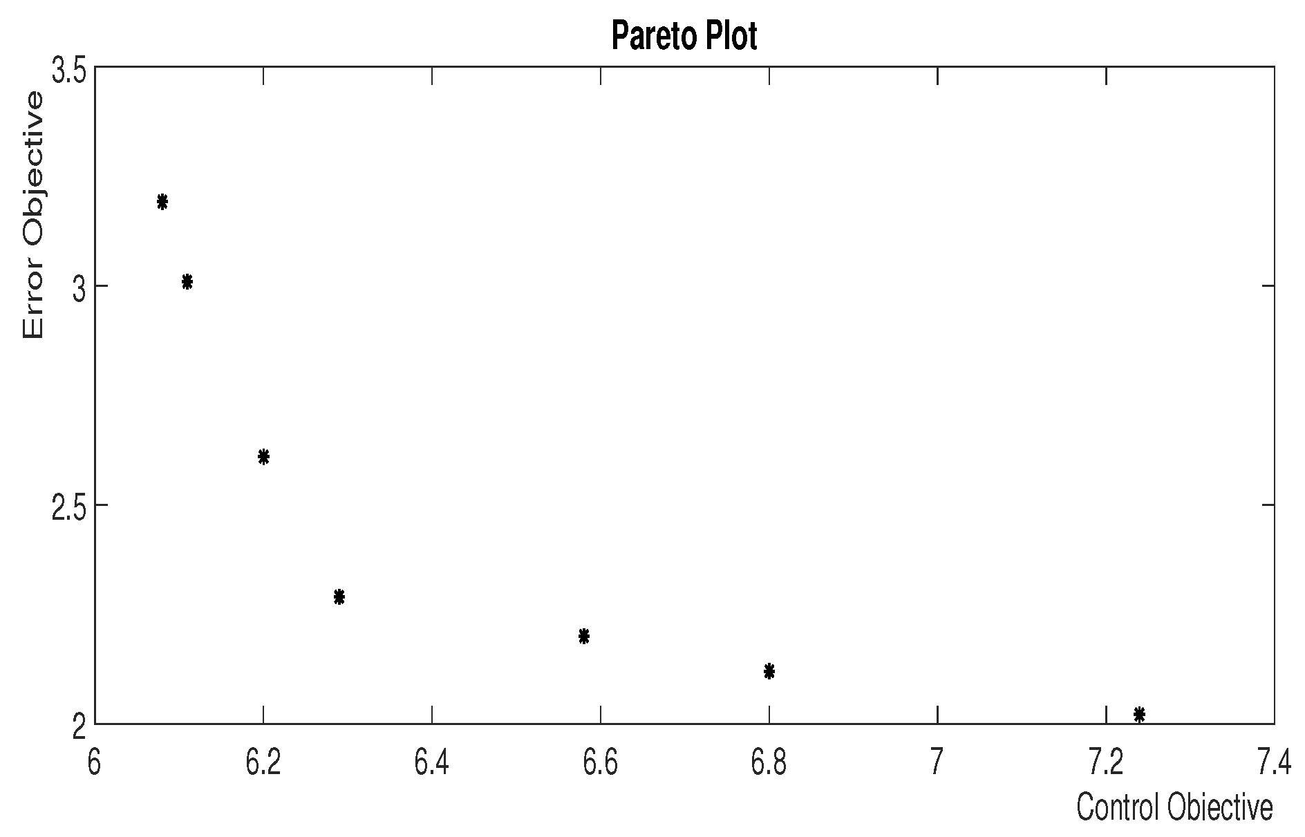
5.1. Problem Statement

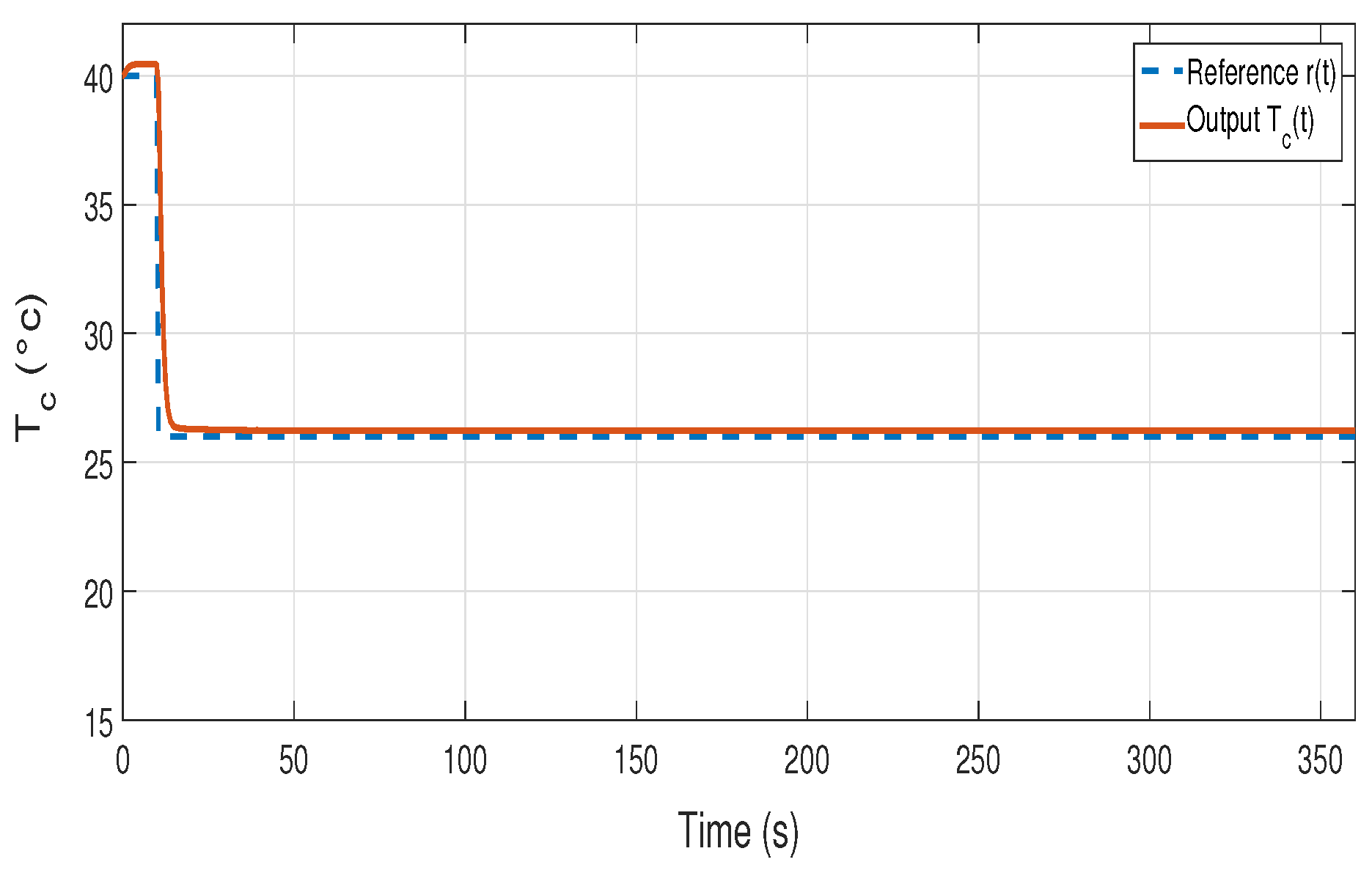
Figure 10 shows a real evolution of cell temperature in the real setup at the CRTEn laboratory (Tunisia). This figure shows how the cell temperature varies with the hour of the day in the function of ambient temperature ($T_a$) and solar radiation (G) presented in Figure 2 and Figure 3. This behaviour has also been reproduced with the thermal model (17) using the same data for $T_a$ and G.

On the other hand, Figure 11 shows the variation of the electric power during the day based on the real values of the solar radiation (see Figure 2). This variation depends also on the cell temperature. When this temperature increases, the electric power will decrease. Therefore, the control of this temperature to its optimal value is a key issue in order to extract the maximum electric power $P_e$ and to guarantee the optimal operation of PV cells. The cell temperature can be reduced by manipulating the water flow rate $\dot{m}$ that circulates in the absorber as can be observed in Figure 6.

In this section, we will propose a solution to the problem related to decreasing PV cell efficiency because of increasing cell temperature. As already discussed, as solar radiance and ambient temperature increase, the temperature of PV cells gradually increases, decreasing the efficiency of the PV cell and consequently decreasing the electrical power $P_e$.

The proposed solution is based on designing an optimal LQR LPV state feedback controller that maintains the cells’ temperature $T_c$ around 25 ${}^{°}$C by manipulating the flow rate of water $\dot{m}$ that circulates in the absorber. This temperature allows the establishment of the standard operating conditions suggested by the manufacturer to obtain the optimal efficiency of the PV cell.

The proposed LPV controller strategy is developed using the polytopic LPV thermal model (24) which takes into account the parameter variation (20)–(23) in the function of the ambient temperature $T_a$ and the glass cover temperature $T_v$.

This controller is similar to a standard state feedback controller but the feedback gain $K\left(\theta \right)$ varies with the varying parameters (20)–(23) in order to guarantee maximum electrical power P for each solar radiation G and ambient temperature $T_a$. The LPV state feedback controller provides the following control action which corresponds to the manipulated water flow rate $\dot{m}$ in the absorber

$$u\left(t\right)=-K\left(\theta \right)x\left(t\right)$$

(29)

where

$$K\left(\theta \right)=\sum _{i=1}^N{\nu }_i\left(\theta \right)K_i$$

(30)

such that the closed-loop system is given by

$$\dot{x}\left(t\right)=\sum _{i=1}^N{\nu }_i\left(\theta \right)(A_i-B{K}_i)x\left(t\right)$$

(31)

The design of the controller gains $K_i$ associated with the vertices of the polytopic model (24) is based on formulating the LQR optimal control problem in LMI form as presented in the next section.

5.2. LMI Method

The optimal $K_i$ will be obtained by rewriting the Ricatti equation associated with the LQR problem

$${(A_i-B{K}_i)}^{T}P+P(A_i-B{K}_i)+Q+K_i^{T}R{K}_i<0$$

(32)

in LMI form.

To do so, we will right multiply (32) by $Y=P^{-1}$ and introduce the following change of variables:

$$\begin{array}{cc}\hfill W_i& =K_{i}Y\hfill \end{array}$$

(33)

$$\begin{array}{cc}\hfill Q& =H^{T}H\hfill \end{array}$$

(34)

Then, we will apply the Schur lemma and will find the following LMI for the Ricatti Equation (32).

$$\left[\begin{array}{ccc}Y{A}_i^T+AY-B{W}_i-{W_i}^T{B}^T& Y{H}^T& {W_i}^T\\ HY& -I_n& 0\\ W_i& 0& -R^{-1}\end{array}\right]<0$$

(35)

To obtain the optimal $K_i$, we will need to solve the following optimization problem

$$\begin{array}{c}\underset{\gamma ,W_i,Y\ge 0}{min}\hfill \\ \mathrm{subject}\mathrm{to}:\hfill \\ \left[\begin{array}{ccc}Y{A}_i^T+AY-B{W}_i-{W_i}^T{B}^T& Y{H}^T& {W_i}^T\\ HY& -I_n& 0\\ W_i& 0& -R^{-1}\end{array}\right]<0i=1,\cdots ,N\hfill \\ \left[\begin{array}{cc}\gamma I_n& I_n\\ I_n& Y\end{array}\right]>0\hfill \end{array}$$

(36)

Then, after the solution of this problem, the optimal $K_i$ will be obtained as follows:

$$K_i=W_i{Y}^{-1}$$

(37)

The tuning of the LPV LQR controller parameters Q and R is obtained by varying their values and determining the Pareto plot presented in Figure 12 which allows us to determine the parameters that provide the best trade-off between error minimisation (performance) and control effort (energy consumption). The best value for the parameters is achieved in the corner point of the plot presented in Figure 12.

Figure 13 shows the closed-loop response of the PV cell temperature using the designed LPV LQR optimal controller (29). The PV/T system is simulated using the nonlinear model presented in Section 3. In this figure, we can observe that after the application of this controller, the PV cell temperature reaches the optimal value (25 ${}^{°}$C) in a short time. This shows the effectiveness of this controller in terms of regulating the temperature of PV cells around the optimal value.

To show the benefits of using the LPV LQR controller proposed in this paper, it is compared with the results obtained using a classical linear-time invariant (LTI) LQR optimal controller designed with the model linearised around the optimal operating point. This controller has a single controller gain matrix K that will be applied in the whole operating range, different from the LPV LQR controller that uses a set of controllers which are scheduled with the operating point according to (29).

The simulation results obtained with the LTI LQR controller are presented in Figure 14. It can be observed that the LQR controller is not able to exactly reach the steady state value because of the variation of the system matrix A with the operating point (19). This fact motivates the use of the proposed LPV approach.

Figure 15 shows the evolution of the control action u that represents the mass flow rate of water injected by the pump from the water tank to the absorber.

The trade-off between speed of the time-response and energy consumption in the water pump can be established with the LQR weights Q and R, respectively.

Further, a disturbance was added to the PV/T system. Figure 16 shows the evolution of the PV cell temperature proving that the controller is able to adjust the PV cell temperature to the optimum value despite the disturbance.

Finally, from Equations (6) and (7), the electrical power $P_e$ (that corresponds with $P_{pv}$) generated by the PV/T system is equal to

$$\begin{array}{c}\hfill P_e={\eta }_{elec}{S}_{pv}G\end{array}$$

(38)

The evolution of this electrical power after the application of the control to adjust the PV cell temperature to its optimal value is represented in Figure 17.

Figure 17 shows the generation of electrical power when the temperature of the PV cell has been adjusted to an optimal value. According to (7), the PV cell produces the maximum electrical power in this case.

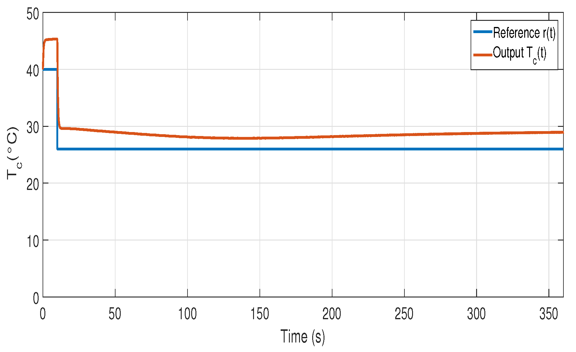
6. State Estimator Design of the PV/T System

To implement the previous controller, we need to have access to all the temperatures of the thermal model (17). However, as discussed in Section 2, the measurements provided by the available sensors only provide the electrical power ($P_e$) and the thermal power ($Q_t$). So, we will need a state estimator that, using the available sensors and the thermal model, will be able to state the temperatures (states) of the PV/T system.

In this section, we will design an optimal state estimator based on an LPV Kalman filter with the LMI method. The considered LPV state estimator has the following structure

$$\begin{array}{cc}\hfill \dot{\widehat{x}}\left(t\right)& =A(\theta \widehat{x}\left(t\right)+Bu\left(t\right)+L\left(\theta \right)(y\left(t\right)-\widehat{y}\left(t\right))\hfill \end{array}$$

(39)

$$\begin{array}{cc}\hfill \widehat{y}\left(t\right)& =C\widehat{x}\left(t\right)\hfill \end{array}$$

(40)

where the gain-scheduled estimator gain $L\left(\theta \right)$ is defined as

$$L\left(\theta \right)=\sum _{i=1}^N{\nu }_i\left(\theta \right)L_i$$

(41)

Obtaining the estimator gains $L_i$ associated to the vertices of the polytopic model (24) is based on formulating the Kalman filter problem in LMI form as presented in the following, considering that the state observer equations can be rewritten as follows:

$$\dot{\widehat{x}}\left(t\right)=(A\left(\theta \right)-L\left(\theta \right)C)\widehat{x}\left(t\right)+Bu\left(t\right)+L\left(\theta \right)y\left(t\right)$$

(42)

Applying the duality principle between control and estimation to the LQR Ricatti Equation (32) ($A_i\to A^T$,$B\to C^T$,$K_i\to L_i^T$), we arrive at

$$\begin{array}{c}\hfill {(A_i^T-C^T{L}_i^T)}^{T}P+P(A_i^T-C^T{L}_i^T)+Q+L_{i}R{L}_i^T<0\end{array}$$

(43)

To express this equation in LMI form, we proceed similarly to the LQR case; we will right multiply (32) by $Y=P^{-1}$ and introduce the following change of variables:

$$\begin{array}{cc}\hfill W_i& =L_i^{T}Y\hfill \end{array}$$

(44)

$$\begin{array}{cc}\hfill Q& =H^{T}H\hfill \end{array}$$

(45)

Then, we will apply the Schur lemma and find the following LMI representation for (43)

$$\left[\begin{array}{ccc}Y{A}_i+A_i^{T}Y-C^T{W}_i-{W_i}^{T}C& Y{H}^T& {W_i}^T\\ HY& -I_n& 0\\ W_i& 0& -R^{-1}\end{array}\right]<0$$

(46)

Finally, to obtain the optimal $L_i$ we will need to solve the following optimization problem

$$\begin{array}{c}\underset{\gamma ,W_i,Y\ge 0}{min}\hfill \\ \mathrm{subject}\mathrm{to}:\hfill \\ \left[\begin{array}{ccc}Y{A}_i+A_i^{T}Y-C^T{W}_i-{W_i}^{T}C& Y{H}^T& {W_i}^T\\ HY& -I_n& 0\\ W_i& 0& -R^{-1}\end{array}\right]<0i=1,\cdots ,N\hfill \\ \left[\begin{array}{cc}\gamma I_n& I_n\\ I_n& Y\end{array}\right]>0\hfill \end{array}$$

(47)

Then, after the solution of this problem, the optimal $L_i$ will be obtained as follows:

$$L_i=Y^{-1}{W}_i$$

(48)

Figure 18 shows the response of the closed-loop system when the LPV Kalman-based state observer, designed using the previous procedure, is used to estimate the states. Comparing this response with the one presented in Figure 12, we can see that it is identical to the one obtained using the LPV state feedback controller considering all states measured. This validates the merit of the proposed state estimation scheme.

7. Conclusions

In this work, the modeling and control of a hybrid PV/T water system in the linear parameter varying (LPV) framework has been proposed. First, the physical model of this PV/T hybrid system was presented. Then, a control-oriented model was derived by transforming the physical nonlinear model into an LPV representation. Using this representation in polytopic form, an optimal LQR LPV state feedback controller was designed using the LMI method. The obtained controller was implemented and tested in simulation, taking into account the disturbance presented by the solar radiation and the ambient temperature during the day. The main goal of this controller is to regulate the PV cell temperature to an optimal value in order to guarantee the extraction of the maximum electrical power. Additionally, a state estimator scheme based on an LPV Kalman filter is proposed to estimate the temperatures of the different layers from the available sensors. The obtained results prove that the optimal LQR LPV state feedback controller not only successfully avoids the problem of temperature increase in PV cells, allowing the PV/T system to extract the maximum electrical energy, but also offers better performance and improvement in higher energy production despite external disturbances. As part of future work, the proposed approach will be tested in the real setup available in the CRTEn laboratory.

References

1. Geller, H.; Schaeffer, R.; Szklo, A.; Tolmasquim, M. Policies for advancing energy efficiency and renewable energy use in Brazil. Energy Policy 2004, 32, 1437–1450. [Google Scholar] [CrossRef]
2. Carrasco, J.M.; Franquelo, L.G.; Bialasiewicz, J.T.; Galván, E.; PortilloGuisado, R.C.; Prats, M.M.; León, J.I.; Moreno-Alfonso, N. Power-electronic systems for the grid integration of renewable energy sources: A survey. IEEE Trans. Ind. Electron. 2006, 53, 1002–1016. [Google Scholar] [CrossRef]
3. Hammons, T.J. Integrating renewable energy sources into European grids. Int. J. Electr. Power Energy Syst. 2008, 30, 462–475. [Google Scholar] [CrossRef]
4. Nie, S.; Huang, C.Z.; Huang, G.; Li, Y.; Chen, J.; Fan, Y.; Cheng, G. Planning renewable energy in electric power system for sustainable development under uncertainty–A case study of Beijing. Appl. Energy 2016, 162, 772–786. [Google Scholar] [CrossRef]
5. Parida, B.; Iniyan, S.; Goic, R. A review of solar photovoltaic technologies. Renew. Sustain. Energy Rev. 2011, 15, 1625–1636. [Google Scholar] [CrossRef]
6. Shadmand, M.B.; Balog, R.S.; Abu-Rub, H. Model predictive control of PV sources in a smart DC distribution system: Maximum power point tracking and droop control. IEEE Trans. Energy Convers. 2014, 29, 913–921. [Google Scholar] [CrossRef]
7. Zhang, P.; Wang, Y.; Xiao, W.; Li, W. Reliability evaluation of grid-connected photovoltaic power systems. IEEE Trans. Sustain. Energy 2012, 3, 379–389. [Google Scholar] [CrossRef]
8. Denis, G.S.; Parker, P. Community energy planning in Canada: The role of renewable energy. Renew. Sustain. Energy Rev. 2009, 13, 2088–2095. [Google Scholar] [CrossRef]
9. Micheli, S. Policy strategy cooperation in the 2030 climate and energy policy framework. Atl. Econ. J. 2020, 48, 265–267. [Google Scholar] [CrossRef]
10. Dimitrov, R.S. The Paris agreement on climate change: Behind closed doors. Glob. Environ. Politics 2016, 16, 1–11. [Google Scholar] [CrossRef]
11. Magagna, D.; Uihlein, A. Ocean energy development in Europe: Current status and future perspectives. Int. J. Mar. Energy 2015, 11, 84–104. [Google Scholar] [CrossRef]
12. Tripanagnostopoulos, Y.; Nousia, T.; Souliotis, M.; Yianoulis, P. Hybrid photovoltaic/thermal solar systems. Sol. Energy 2002, 72, 217–234. [Google Scholar] [CrossRef]
13. Slimani, M.E.A.; Amirat, M.; Bahria, S.; Kurucz, I.; Sellami, R. Study and modeling of energy performance of a hybrid photovoltaic/thermal solar collector: Configuration suitable for an indirect solar dryer. Energy Convers. Manag. 2016, 125, 209–221. [Google Scholar] [CrossRef]
14. Jendoubi, A.; Tlili, F.; Bacha, F. Sliding mode control for a grid connected PV-system using interpolation polynomial MPPT approach. Math. Comput. Simul. 2020, 167, 202–218. [Google Scholar] [CrossRef]
15. Mahamudul, H.; Rahman, M.M.; Metselaar, H.; Mekhilef, S.; Shezan, S.; Sohel, R.; Abu Karim, S.B.; Badiuzaman, W.N.I. Temperature regulation of photovoltaic module using phase change material: A numerical analysis and experimental investigation. Int. J. Photoenergy 2016, 2016, 5917028. [Google Scholar] [CrossRef]
16. Khalid, M.; Shanks, K.; Ghosh, A.; Tahir, A.; Sundaram, S.; Mallick, T.K. Temperature regulation of concentrating photovoltaic window using argon gas and polymer dispersed liquid crystal films. Renew. Energy 2021, 164, 96–108. [Google Scholar] [CrossRef]
17. Ceylan, I.; Gürel, A.E.; Demircan, H.; Aksu, B. Cooling of a photovoltaic module with temperature controlled solar collector. Energy Build. 2014, 72, 96–101. [Google Scholar] [CrossRef]
18. Haidar, Z.A.; Orfi, J.; Kaneesamkandi, Z. Photovoltaic panels temperature regulation using evaporative cooling principle: Detailed theoretical and real operating conditions experimental approaches. Energies 2020, 14, 145. [Google Scholar] [CrossRef]
19. Pang, W.; Cui, Y.; Zhang, Q.; Yu, H.; Zhang, X.; Zhang, Y.; Yan, H. Comparative investigation of performances for HIT-PV and PVT systems. Sol. Energy 2019, 179, 37–47. [Google Scholar] [CrossRef]
20. Taguchi, M.; Yano, A.; Tohoda, S.; Matsuyama, K.; Nakamura, Y.; Nishiwaki, T.; Fujita, K.; Maruyama, E. 24.7% record efficiency HIT solar cell on thin silicon wafer. IEEE J. Photovoltaics 2013, 4, 96–99. [Google Scholar] [CrossRef]
21. Garg, H.; Adhikari, R.S. Conventional hybrid photovoltaic/thermal (PV/T) air heating collectors: Steady-state simulation. Renew. Energy 1997, 11, 363–385. [Google Scholar] [CrossRef]
22. Herrando, M.; Ramos, A. Photovoltaic-Thermal (PV-T) Systems for Combined Cooling, Heating and Power in Buildings: A Review. Energies 2022, 15, 3021. [Google Scholar] [CrossRef]
23. Omer, K.A.; Zala, A.M. Experimental investigation of PV/thermal collector with theoretical analysis. Renew. Energy Focus 2018, 27, 67–77. [Google Scholar] [CrossRef]
24. Fiorentini, M.; Cooper, P.; Ma, Z.; Robinson, D.A. Hybrid model predictive control of a residential HVAC system with PVT energy generation and PCM thermal storage. Energy Procedia 2015, 83, 21–30. [Google Scholar] [CrossRef]
25. Fudholi, A.; Razali, N.F.M.; Ridwan, A.; Yendra, R.; Hartono, H.; Desvina, A.P.; Majahar, M.K.B.; Sopian, K. Overview of photovoltaic thermal (PVT) water collector. Int. J. Power Electron. Drive Syst. 2018, 9, 1891. [Google Scholar] [CrossRef]
26. Jia, Y.; Alva, G.; Fang, G. Development and applications of photovoltaic–thermal systems: A review. Renew. Sustain. Energy Rev. 2019, 102, 249–265. [Google Scholar] [CrossRef]
27. Haurant, P.; Ménézo, C.; Gaillard, L.; Dupeyrat, P. Modélisation numérique d’un système hybride photovoltaïque/thermique intégré à un chauffe-eau solaire. In Proceedings of the 3ième Colloque International Francophone d’Energétique et Mécanique Les énergies renouvelables et la mécanique appliquée à l’industrie, Mororni, Comores, 1 January 2014; p. ART–4. [Google Scholar]
28. Welch, R.L.; Venayagamoorthy, G.K. Energy dispatch fuzzy controller for a grid-independent photovoltaic system. Energy Convers. Manag. 2010, 51, 928–937. [Google Scholar] [CrossRef]
29. Slotine, J.J.E. Sliding controller design for non-linear systems. Int. J. Control 1984, 40, 421–434. [Google Scholar] [CrossRef]
30. Kalla, U.K.; Singh, B.; Murthy, S.S.; Jain, C.; Kant, K. Adaptive sliding mode control of standalone single-phase microgrid using hydro, wind, and solar PV array-based generation. IEEE Trans. Smart Grid 2017, 9, 6806–6814. [Google Scholar] [CrossRef]
31. Sira-Ramirez, H. On the dynamical sliding mode control of nonlinear systems. Int. J. Control 1993, 57, 1039–1061. [Google Scholar] [CrossRef]
32. Singh, S.; Agarwal, S.; Tiwari, G.; Chauhan, D. Application of genetic algorithm with multi-objective function to improve the efficiency of glazed photovoltaic thermal system for New Delhi (India) climatic condition. Sol. Energy 2015, 117, 153–166. [Google Scholar] [CrossRef]
33. Ravaee, H.; Farahat, S.; Sarhaddi, F. Artificial neural network based model of photovoltaic thermal (pv/t) collector. J. Math. Comput. Sci. 2012, 4, 411–417. [Google Scholar] [CrossRef]
34. Ammar, M.B.; Chaabene, M.; Chtourou, Z. Artificial neural network based control for PV/T panel to track optimum thermal and electrical power. Energy Convers. Manag. 2013, 65, 372–380. [Google Scholar] [CrossRef]
35. M’zoughi, F.; Garrido, A.J.; Garrido, I.; Bouallègue, S.; Ayadi, M. Sliding mode rotational speed control of an oscillating water column-based wave generation power plants. In Proceedings of the 2018 International Symposium on Power Electronics, Electrical Drives, Automation and Motion (SPEEDAM), Amalfi, Italy, 20–22 June 2018; IEEE: Hoboken, NJ, USA, 2018; pp. 1263–1270. [Google Scholar]
36. Singh, S.; Agrawal, S.; Tiwari, A.; Al-Helal, I.; Avasthi, D. Modeling and parameter optimization of hybrid single channel photovoltaic thermal module using genetic algorithms. Sol. Energy 2015, 113, 78–87. [Google Scholar] [CrossRef]
37. Jarimi, H.; Bakar, M.N.A.; Othman, M.; Din, M.H. Bi-fluid photovoltaic/thermal (PV/T) solar collector: Experimental validation of a 2-D theoretical model. Renew. Energy 2016, 85, 1052–1067. [Google Scholar] [CrossRef]
38. Naderi, E.; Asrari, A. Experimental validation of grid-tied and standalone inverters on a lab-scale wind-PV microgrid. In Proceedings of the 2021 IEEE International Power and Renewable Energy Conference (IPRECON), Kollam, India, 24–26 September 2021; IEEE: Hoboken, NJ, USA, 2021; pp. 1–6. [Google Scholar]
39. JAMAAOUI, F.; AYADI, M.; Vicenç, P. Comparative study between Experimental and Simulation results of a PV/T water panel. In Proceedings of the 2020 11th International Renewable Energy Congress (IREC), Hammamet, Tunisia, 29–31 October 2020; IEEE: Hoboken, NJ, USA, 2020; pp. 1–5. [Google Scholar]
40. Jamaaoui, F.; Ayadi, M.; Puig, V. Influence of a water flow variation on the efficiency of a hybrid PV/T water panel. In Proceedings of the 2020 7th International Conference on Control, Decision and Information Technologies (CoDIT), Prague, Czech Republic, 29 June–2 July 2020; IEEE: Hoboken, NJ, USA, 2020; Volume 1, pp. 277–281. [Google Scholar]
41. Yin, H.; Yang, D.; Kelly, G.; Garant, J. Design and performance of a novel building integrated PV/thermal system for energy efficiency of buildings. Sol. Energy 2013, 87, 184–195. [Google Scholar] [CrossRef]
42. Nasir, F.H.; Husaini, Y. MATLAB simulation of photovoltaic and photovoltaic/thermal systems performance. In Proceedings of the IOP Conference Series: Materials Science and Engineering; IOP Publishing: Bristol, UK, 2018; Volume 341, p. 012019. [Google Scholar]
43. Solanki, S.; Dubey, S.; Tiwari, A. Indoor simulation and testing of photovoltaic thermal (PV/T) air collectors. Appl. Energy 2009, 86, 2421–2428. [Google Scholar] [CrossRef]
44. Rejeb, O.; Dhaou, H.; Jemni, A. A numerical investigation of a photovoltaic thermal (PV/T) collector. Renew. Energy 2015, 77, 43–50. [Google Scholar] [CrossRef]
45. Sarhaddi, F.; Farahat, S.; Ajam, H.; Behzadmehr, A.; Adeli, M.M. An improved thermal and electrical model for a solar photovoltaic thermal (PV/T) air collector. Appl. Energy 2010, 87, 2328–2339. [Google Scholar] [CrossRef]
46. Kwiatkowski, A.; Boll, M.T.; Werner, H. Automated generation and assessment of affine LPV models. In Proceedings of the 45th IEEE Conference on Decision and Control, San Diego, CA, USA, 13–15 December 2006; IEEE: Hoboken, NJ, USA, 2006; pp. 6690–6695. [Google Scholar]
47. Apkarian, P.; Gahinet, P.; Becker, G. Self-scheduled H control of linear parameter-varying systems: A design example. Automatica 1995, 31, 1251–1261. [Google Scholar] [CrossRef]
Figure 1. (a) Hybrid PV/T system type VOLTHER PowerTherm in the CRTEn laboratory. (b) Hybrid PV/T system schematic diagram.
Processes 11 03426 g001
Figure 2. Real solar radiation data in CRTEn laboratory.
Processes 11 03426 g002
Figure 3. Real ambient temperature data in CRTEn laboratory.
Processes 11 03426 g003
Figure 4. Conceptual representation of the covered hybrid PV/T water system.
Processes 11 03426 g004
Figure 5. Electrical model of a PV cell.
Processes 11 03426 g005
Figure 6. Interpolation functions ν 1 , ν 2 , ν 3 , ν 4 of the polytopic LPV model.
Processes 11 03426 g006
Figure 7. Interpolation functions ν 5 , ν 6 , ν 7 , ν 8 of the polytopic LPV model.
Processes 11 03426 g007
Figure 8. Interpolation functions ν 9 , ν 10 , ν 11 , ν 12 of the polytopic LPV model.
Processes 11 03426 g008
Figure 9. Interpolation functions ν 13 , ν 14 , ν 15 , ν 16 of of the polytopic LPV model.
Processes 11 03426 g009
Figure 10. Real variation of cell temperature by varying time and water flow rate.
Processes 11 03426 g010
Figure 11. Variation of the electrical power.
Processes 11 03426 g011
Figure 12. Tuning control parameters using the Pareto plot.
Processes 11 03426 g012
Figure 13. PV cell temperature ( T c ) applying the LQR LPV controller (without disturbance).
Processes 11 03426 g013
Figure 14. Evolution of the PV cell temperature ( T c ) with LQR controller.
Processes 11 03426 g014
Figure 15. Control action u ( t ) .
Processes 11 03426 g015
Figure 16. PV cell temperature ( T c ) applying the LQR LPV controller (with disturbance).
Processes 11 03426 g016
Figure 17. Electrical power obtained using the proposed LPV LQR controller.
Processes 11 03426 g017
Figure 18. PV cell temperature T c of polytopic LPV system with observer.
Processes 11 03426 g018