Article

Reduced-Order Modeling and Control of Heat-Integrated Air Separation Column Based on Nonlinear Wave Theory

College of Control Science and Engineering, China University of Petroleum (East China), Qingdao 266580, China
*
Author to whom correspondence should be addressed.
Processes 2023, 11(10), 2918; https://doi.org/10.3390/pr11102918
Submission received: 7 September 2023 / Revised: 28 September 2023 / Accepted: 3 October 2023 / Published: 5 October 2023
(This article belongs to the Special Issue Green Separation and Purification Processes)

Abstract

:
The process of low-temperature air separation consumes a significant amount of energy. Internal heat-integrated distillation technology has considerable energy-saving potential. Therefore, the combination of low-temperature air separation and heat-integrated distillation technology has led to the development of a heat-integrated air separation column (HIASC). Due to the heat integration and the inherent complexity of air separation, the modeling and control of this process poses significant challenges. This paper first introduces the nonlinear wave theory into the HIASC, derives the expression for the velocity of the concentration distribution curve movement and the curve describing function, and then establishes a nonlinear wave model. Compared to the traditional mechanical models, this approach greatly reduces the number of differential equations and variables while ensuring an accurate description of the system characteristics. Subsequently, based on the wave model, a model predictive control scheme is designed for the HIASC. This scheme is compared with two conventional control schemes: PID and a general model control. The simulation results demonstrate that MPC outperforms the other control schemes from the response curves and performance metrics.

1. Introduction

Air separation is the process of separating the main components of air based on the differences in their physical properties. The oxygen, nitrogen, chlorine, and other gases produced by air separation equipment have wide applications in the national economy [1,2,3,4]. The cryogenic air separation is a primary approach for obtaining high-purity gases like nitrogen, oxygen, and argon. The raw material for cryogenic air separation units is atmospheric air, and their primary energy consumption comes from electricity, accounting for over 70% of the production cost [4,5,6,7]. Particularly, as environmental concerns intensify, the demand for energy efficiency and emission reduction is increasing [8,9]. Therefore, reducing energy consumption in air separation units has become especially crucial.
The primary working principle of cryogenic air separation technology involves compressing and liquefying air, removing impurities, and cooling it. The desired products are obtained through a specialized distillation column, known as the air separation column, by utilizing the different boiling points of various components. This air separation process is essentially a specific form of cryogenic distillation. In the cryogenic air separation process, the distillation column serves as a crucial mass transfer unit operation and represents the primary energy-consuming unit. Most of the energy in the air separation process is utilized for the distillation and separation processes, with only a small portion used to produce specific gas products. Therefore, researching energy-saving solutions for this distillation process holds significant economic and societal importance [10].
Among numerous distillation energy-saving technologies, heat-integrated distillation technology has garnered extensive attention due to its significant potential for energy savings [11,12,13,14]. In heat-integrated distillation technology, the rectifying section and the stripping section are two separate columns, referred to as the rectifying column and the stripping tower, respectively [15,16,17,18,19]. These columns are connected by a compressor and a throttle valve to regulate the pressure between them. Heat exchangers are placed between the rectifying and stripping columns to achieve thermal coupling. This arrangement significantly enhances energy utilization, leading to energy savings of over 30% compared to the conventional distillation processes. The energy-saving effect of internal heat integration in the distillation process is pronounced, and since air separation is a specific form of cryogenic distillation, introducing heat integration technology into the air separation process holds vital significance. Additionally, traditional cryogenic distillation in air separation involves a high-pressure tower and a low-pressure tower, with existing single-plate coupling between the bottoms of the high-pressure column and the tops of the low-pressure column. Therefore, the practical applicability of heat integration technology in air separation is further evident [20,21,22]. Currently, some scholars have made progress in the design and optimization of HIASCs [23,24,25,26]. However, due to the unique thermal coupling structure, challenges arise in the dynamic modeling, control scheme design, and other aspects [27,28].
The dynamic modeling and corresponding control scheme design are crucial and challenging aspects of the distillation and air separation processes. The complexity increases when dealing with systems that incorporate the unique structure of internal heat coupling and the demand for high-purity and ultra-high-purity products. In recent years, wave theory has played a significant role in nonlinear dynamic modeling and control scheme design for separation processes, capturing the attention of scholars [29,30]. In the concept of wave theory for separation processes, certain physical quantities, such as the concentration and temperature distributions of the components, exhibit a constant waveform that propagates towards new steady-state positions during the dynamic separation processes. This phenomenon serves as a tool to explain and describe the nonlinear and dynamic characteristics of complex separation processes simply and accurately. For distillation and air separation processes, researchers like Luyben [31,32,33] and Hwang [34,35,36,37,38] have conducted extensive studies that demonstrated how different steady states of a distillation column can be described using different constant waveform positions. When the setpoint of the distillation column changes or external disturbances disrupt the system’s steady state, the constant waveform will propagate and move within the column until the distillation column reaches a new steady state. The waveform propagation within the column offers a fresh perspective on the nonlinear dynamic process of distillation columns, opening up new possibilities for establishing nonlinear dynamic models for distillation and air separation processes. Moreover, several control scheme performances have been enhanced to some extent based on the wave model. Some researchers have explored the integration of control schemes and wave theory, achieving certain levels of success in this endeavor [39,40,41].
However, when it comes to the HIASC, the complexity of the thermal coupling structure combined with the non-ideal nature of multicomponent air mixtures results in even more unique dynamic characteristics. Strong nonlinearities and other complex features make capturing the dynamic behavior even more challenging. Moreover, applying wave theory to the context of HIASCs requires a re-derivation of the relevant wave equations. There are relatively few reports regarding MPCs for a HIASC based on the wave model. We analyze the main reason for this is that, since many parameters need real-time estimation through live data, the wave model, although more accurate, exhibits a relatively unstable error direction. This can lead to control instability in error-compensating control schemes like MPCs. Furthermore, compared to other control schemes, MPCs exhibit less reliance on the model structure and is more suitable for solving constrained control problems.
A re-modeling study of the HIASC is conducted based on the wave theory in this work. This involves discarding the assumptions of constant molar flow and waveform velocity typically used in traditional distillation process models. This approach aims to align the model more accurately with the characteristics of the heat-coupled air separation process. Simultaneously, by leveraging the constructed wave model, a nonlinear model predictive control scheme is proposed. This scheme is compared with traditional control approaches like PID and general model control. The simulation results indicate that the proposed control scheme outperforms the other two approaches in terms of the control performance.

2. Wave Modeling of the HIASC

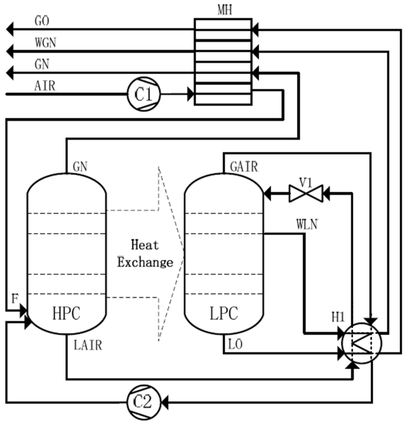
2.1. The Mechanism Model of the HIASC

The HIASC structure used in this study is illustrated in Figure 1. The feed compressed air (AIR) and the gas products generated from the air separation undergo heat exchange in the main heat exchanger (MH), allowing the feed stream to be pre-cooled. The compressed and cooled stream F is introduced as the feed at the bottom of the high-pressure column. Oxygen-rich liquid air (LAIR) flows through the heat exchanger (H1) and enters the top of the low-pressure column through a throttle valve (V1), providing a downward liquid phase flow. Oxygen-rich vapor air (GAIR) at the top of the low-pressure column follows the opposite path, flowing into the high-pressure column and providing an upward gas phase flow. A low-purity liquid nitrogen product (WLN) side stream is withdrawn near the argon-rich stage. A compressor (C2) and throttle valve (V1) are installed between the high-pressure and low-pressure columns, allowing the rectifying and stripping sections to operate at different pressures. The rectifying section operates at a higher pressure and temperature, allowing the LAIR stream from the high-pressure column to flow into the low-pressure column and the GAIR stream from the low-pressure column to flow into the high-pressure column. Internal heat coupling is achieved through the full coupling between the high-pressure and low-pressure columns. A certain amount of heat is transferred from each tray of the high-pressure column to the low-pressure tower, providing a downward liquid phase flow for the high-pressure column and an upward gas phase flow for the low-pressure column. This fully heat-coupled structure closely approximates the ideal heat-integrated distillation column configuration with reduced loads on the condenser and reboiler. As a consequence, the fully heat-coupled design offers superior energy efficiency. Specific operating conditions are provided in Table 1. The flow rate represents the flow rate of the feed. The feed stage is the location at which the feed is introduced. The stage number denotes the total number of trays in the column. The side stream stage refers to the location at which the side stream is extracted. Nitrogen and oxygen product purity represent the nitrogen and oxygen concentrations at the column’s two ends under initial steady-state conditions.
According to the principles of material conservation and energy conservation:
d M j x i , j d t = L j 1 x i , j 1 + V j + 1 y i , j + 1 + F j   z i , j ( L j + S L j ) x i , j ( V j + S V j ) y i , j ;
d M j H j L d t = L j 1 H j 1 L + V j + 1 H j + 1 V + F j H j F ( L j + S L j ) H j L ( V j + S V j ) H j V + Q j  
where the subscript “i” represents the component index, with “i = 1” denoting nitrogen, “i = 2” denoting argon, and “i = 3” marking oxygen. The subscript “j” indicates the stage number, where “j = 1” corresponds to the column top and “j = n” corresponds to the column bottom. The subscript “V” represents the gas phase, “L” denotes the liquid phase, and “F” represents the feed. The variables “M” represent the holdup of liquid on a tray, “L” and “V” represent the molar flow rates of gas and liquid phases, respectively, “SL” and “SV” represent the molar flow rates of liquid and gas phases for the side stream, respectively. The variable “F” stands for the feed flow rate, “H” represents the enthalpy value, “x” is the liquid phase component concentration, “y” is the gas phase component concentration, “z” is the molar fraction of the feed component, and “Q” represents the coupling heat between the rectification and stripping sections. The material conservation and energy conservation equations, combined with the gas–liquid equilibrium equation, concentration summation equation, heat coupling equation, and gas–liquid flow rate equation, constitute the mechanism model of HIASC. The mechanism model employs modeling methods from the literature [23] as a foundation for subsequent derivation of the wave model.

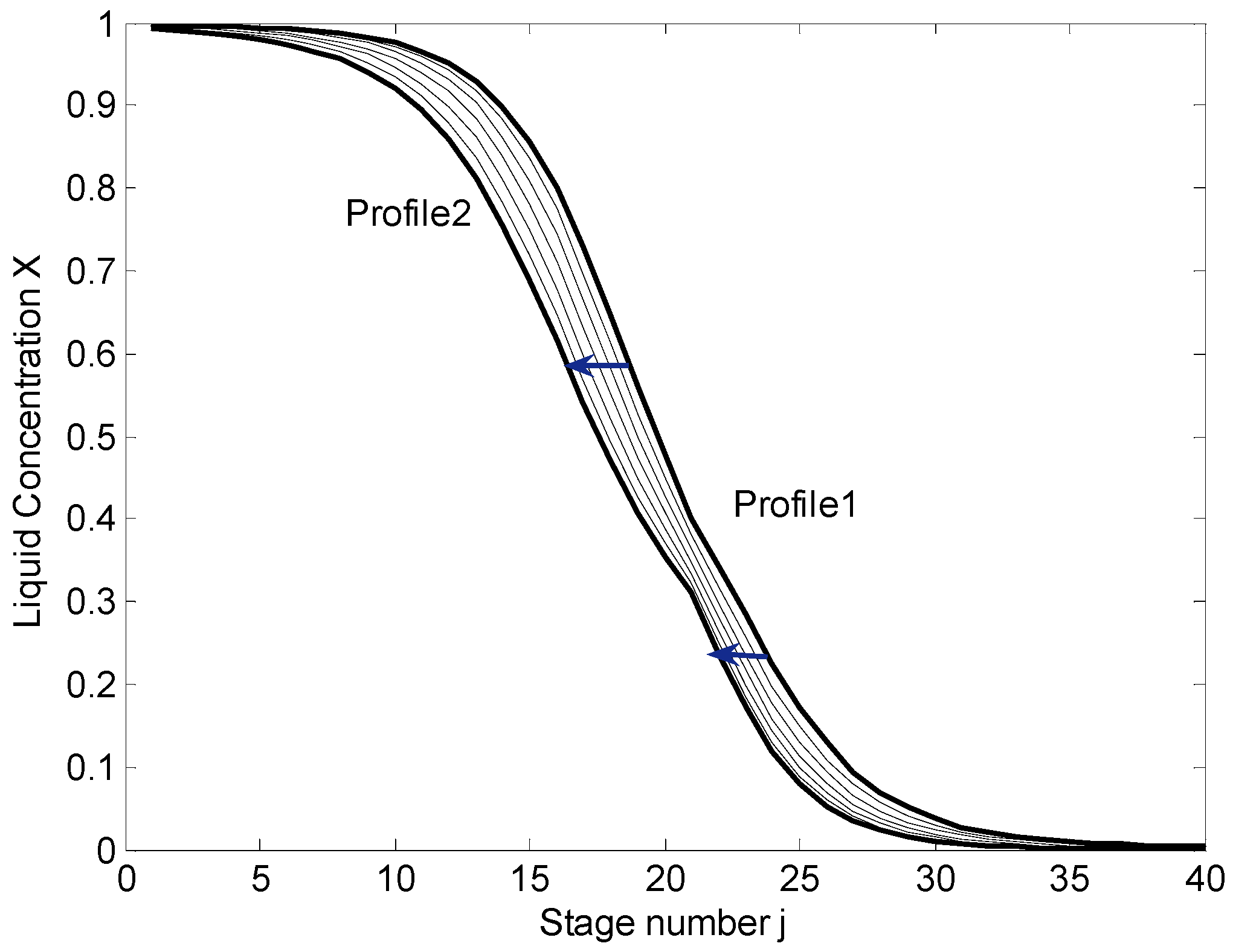
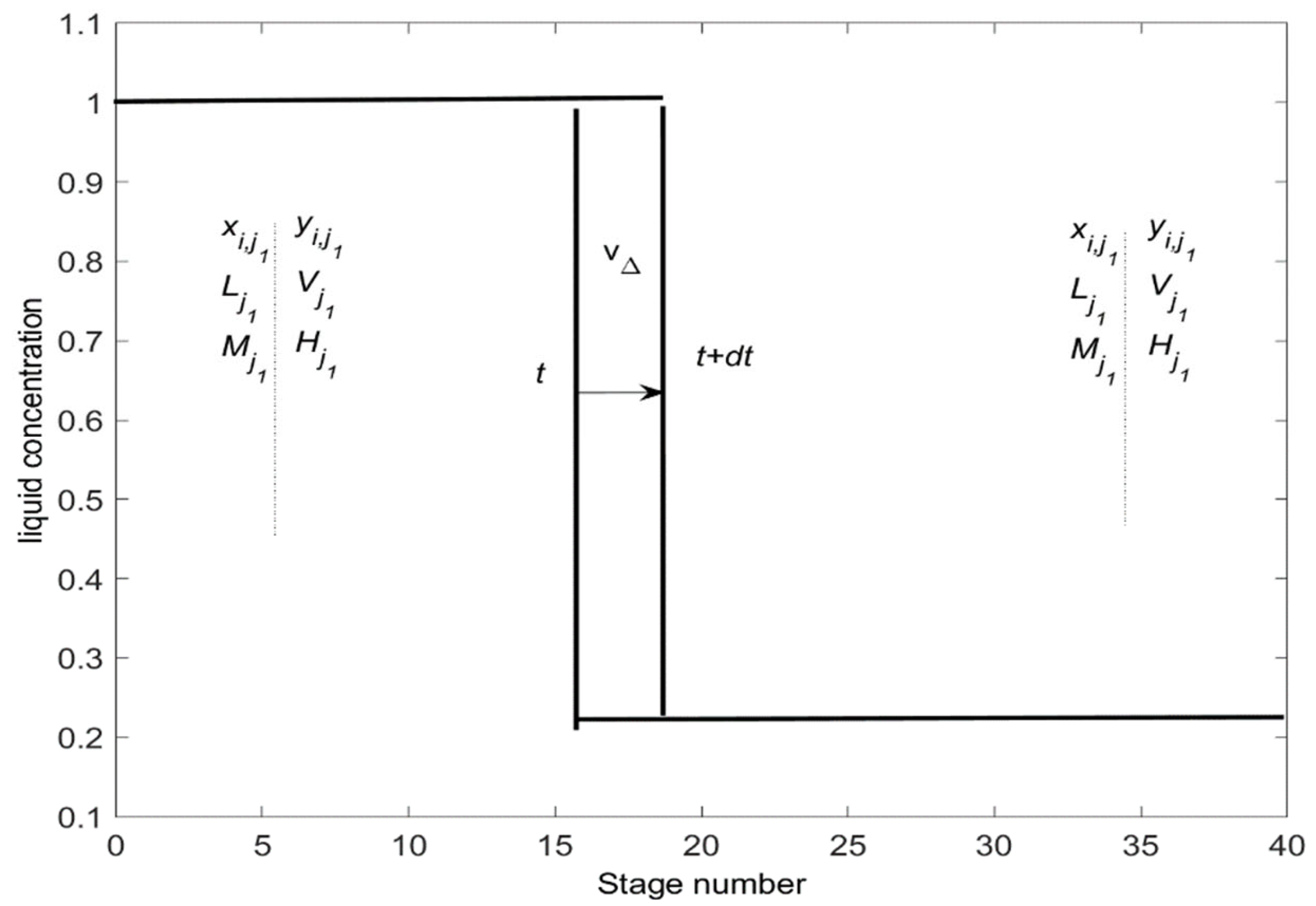
2.2. Wave Modeling of the HIASC
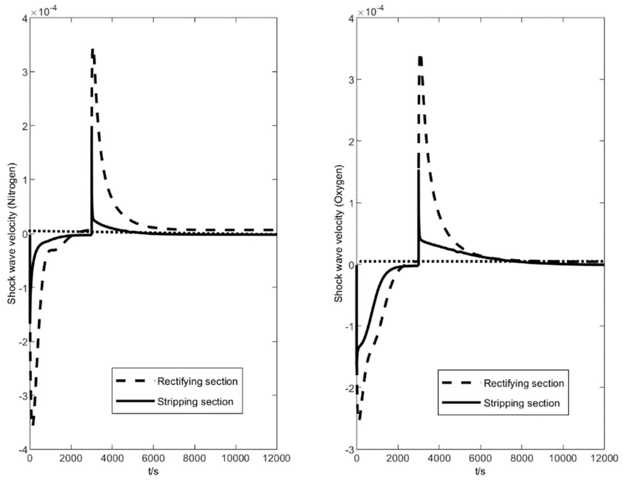
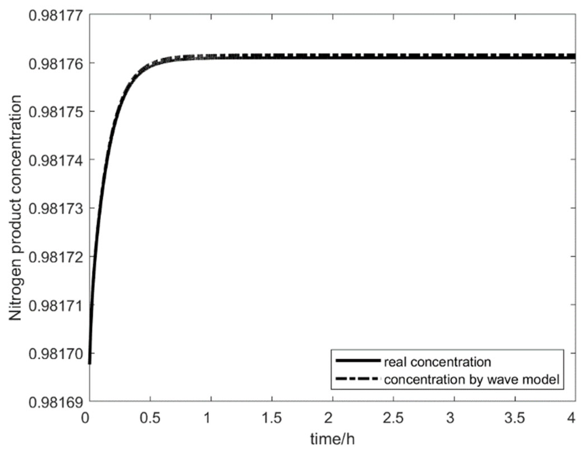
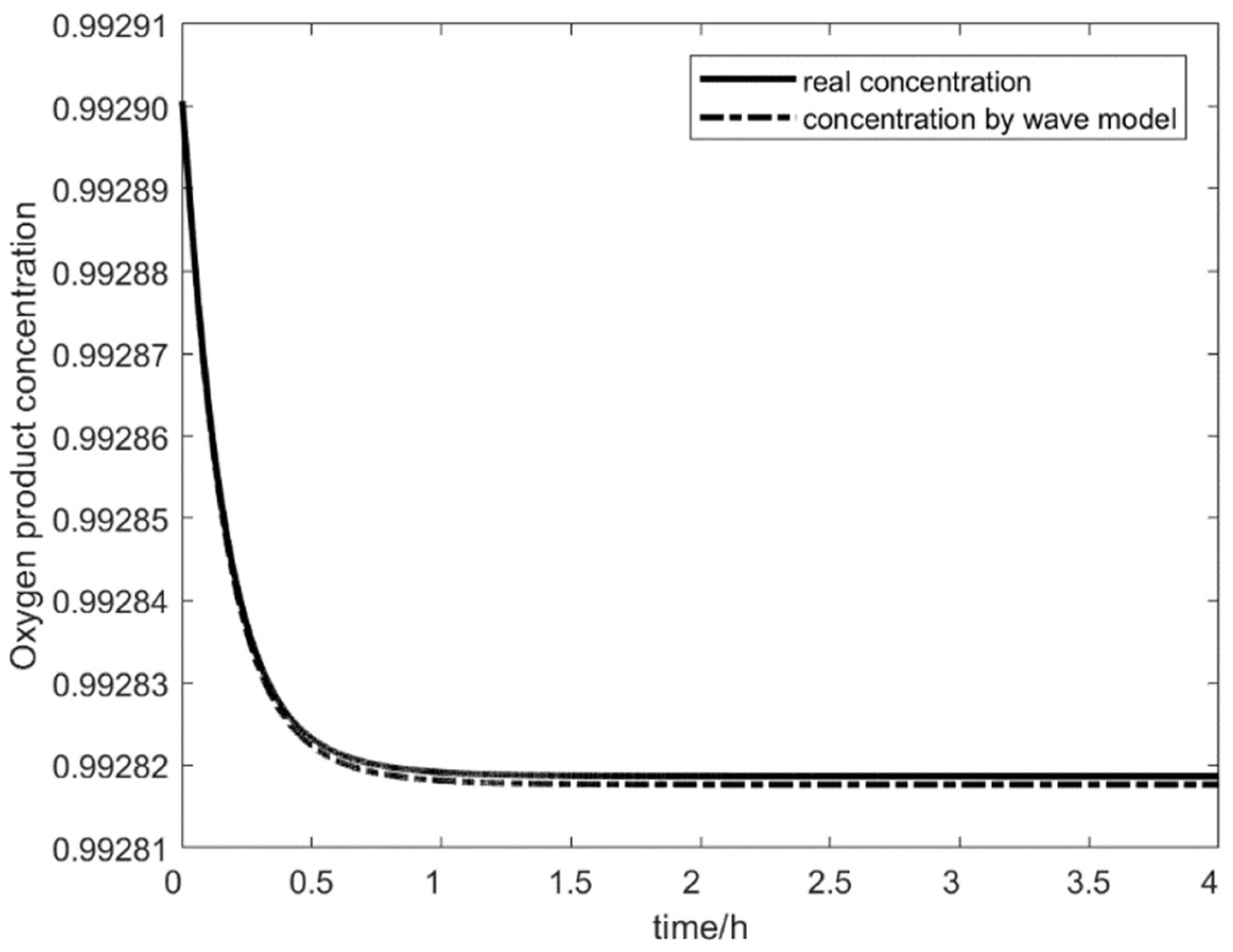
In the wave theory, we treat the concentration distribution curve as a whole to study its behavior. When operational conditions change, the concentration distribution on the trays will also change, resulting in the propagation of the concentration waves through the distillation column. As shown in Figure 2, the original Profile 1 shifts in response to the changing operational conditions, moving within the column. This movement signifies the propagation of the concentration wave within the distillation column, ultimately coming to rest at the position of Profile 2. The location of the waveform in Profile 2 represents the new steady state. The process of Profile 1 moving towards Profile 2, which is the propagation of the concentration wave, represents the dynamic response of the entire system to changes in the operational conditions.
For simplicity, we often choose a specific point on the concentration distribution curve to represent the entire curve, describing its position and movement. This point is referred to as the inflection point and is typically located where the curve has the steepest slope. Given the complexity of the components in the air separation process and the involvement of internal heat coupling, the wave modeling of the HIASC becomes more challenging. This requires us to derive the wave model specifically for the HIASC.
First, according to the material conservation equation Equation (1), we have:
j 1 j 2 d M j x i , j d t d j = ( L j 1 1 x i , j 1 1 + V j 2 + 1 y i , j 2 + 1 + k = j 1 j 2 F k z k ) ( L j 2 x i , j 2 + V j 1 y i , j 1 + k = j 1 j 2 ( S L j 1 X j 1 + S V j 1 y j 1 ) )
where j 1 and j 2 are the two ends of the integration, representing the tray positions at the two ends of the integration. Figure 3 provides a simplified schematic diagram of waveform propagation in the stripping section. Therefore, the integral on the left side of Equation (3) can be approximated as follows:
j 1 j 2 d M j x i , j d t d j = ( M j 1 x i , j 1 M j 2 x i , j 2 ) d j d t
Combining Equations (3) and (4), the wave propagation velocity expression is obtained as follows:
d S d t Δ x i , j = ( L j 1 1 x i , j 1 1 + V j 2 + 1 y i , j 2 + 1 + k = j 1 j 2 F k z k ) ( L j 2 x i , j 2 + V j 1 y i , j 1 + k = j 1 j 2 ( S L k x k + S V k y k ) ) M j 1 x i , j 1 M j 2 x i , j 2
where “S” represents the inflection point position of the integrated segment waveform, indicating the location of the integrated segment waveform.
Similarly, according to Equation (2), we can derive the following expression for the wave velocity:
d S d t Δ H j L = ( L j 1 1 H j 1 1 L + V j 2 + 1 H j 2 + 1 V + k = j 1 j 2 F k H k F ) ( L j 2 H j 2 L + V j 1 H j 1 V + k = j 1 j 2 ( S L k H k L + S V k H k V ) ) M j 1 H j 1 L M j 2 H j 2 L
By combining Equations (1) and (3), extending the integration from a local position to the entire waveform, and performing the appropriate algebraic manipulations, the formula for the wave velocity can be derived as follows:
d S d t x i , j = ( L j 1 x i , j 1 + V j + 1 y i , j + 1 + F j z j ) ( L j x i , j + V j y i , j + S L j X j + S V j y j ) ) M j 1 x i , j 1 M j x i , j
After deriving the wave velocity, we can comprehend the situation of component concentration waveforms. To eventually establish the nonlinear wave model, obtaining the actual values of the component concentrations from their waveforms is necessary. A new function is introduced to link the waveform positions with the concentration values. By observing the concentration distribution curve, the overall shape of the curve exhibits an “S” shape. In other words, there is an inflection point in the middle of the curve, and the concentrations at both ends of the curve asymptotically approach a certain straight line. Hence, empirical functions can be used for fitting. Empirical functions with substantial verification in the separation process are introduced for the waveforms of the high-pressure and low-pressure columns [42]:
x ^ i , j = X i , H _ min + X i , H _ max X i , H _ min 1 + e γ i , H ( j S i , H ) , j = 1 , 2 , , n / 2
x ^ i , j = X i , L _ min + X i , L _ max X i , L _ min 1 + e γ i , L ( j S i , L ) , j = n / 2 + 1 , , n
where x ^ i , j represents the estimated liquid concentration obtained through the waveform positions and empirical relationships, X i , H _ min and X i , H _ max denote the asymptotic limits at the extended ends of the high-pressure tower waveform, X i , L _ min and X i , L _ max represent the asymptotic limits at the extended ends of the low-pressure tower waveform, γ i , H and γ i , L are the slopes at the inflection points of the waveforms for the high-pressure column and low-pressure column, respectively, S i , H and S i , L are the inflection point positions of the waveforms for the two columns.
The expression for the gas–liquid equilibrium equation is as follows:
y i , j = k i , j x i , j
where k is the gas–liquid equilibrium coefficient.
The heat coupling equation describes the heat transfer relationship between the rectifying section and the stripping section, and the expression is as follows:
Q j = U o v A Δ T j
where U o v is the heat transfer coefficient, A is the heat transfer area, and Δ T j   is the temperature difference between a pair of heat-coupled trays.
The calculation equation for the gas–liquid equilibrium coefficient is an implicit expression of the tray temperature, pressure, and equilibrium molar fraction, with the specific relationship obtainable through the Peng-Robinson state equation [43]. The expression for the gas–liquid equilibrium coefficient is as follows:
k i , j = k i , j ( x i , j , y i , j , P j , T j )
Due to the involvement of internal heat coupling, the molar flow rates of gas and liquid are no longer assumed to be constant but are considered to vary with tray position. The detailed flow rate relationships are as follows:
L j = Q j λ + L j 1 + F j q j U j
V j = Q j λ + V j + 1 + F j ( 1 q j ) G j
where λ is the latent heat of vaporization and q represents the feed thermal condition. The liquid flow of each tray comprises several components: liquid generated by condensation resulting from heat release, liquid flowing down from the tray above, the liquid portion from the feed, and the liquid portion removed in the side draw. The gas flow exhibits a similar composition. Due to heat exchange, either vaporization or condensation, the gas and liquid phase flows on each tray cannot be considered constant.
The waveform description function characterizes the system’s state at a specific moment, while the wave velocity function describes the system’s dynamic process. Combined with the gas–liquid equilibrium equation, heat coupling equation, and gas–liquid molar flow rate equation, these components can describe both the steady-state and dynamic processes of the heat-integrated air separation process. The above relations establish the nonlinear wave model for the HIASC.

2.3. Model Test

A characteristic nonlinear dynamic behavior in distillation processes is asymmetry. It means that the system transitions rapidly from one steady state to another after a disturbance occurs. However, when reverting the disturbance, the system’s return to the original equilibrium state is much slower than the speed of reaching the new equilibrium state. We can illustrate and explain this nonlinear feature using the wave model. Figure 4 displays the dynamic asymmetry of the HIASC through changes in wave velocity. At the initial moment, with a 10% variation in feed thermal condition, the wave speed of the rectifying and stripping sections reaches zero after 3000 s, and the system reaches a new steady state. At around 8000 s, when the feed thermal condition is restored to its initial value, the wave velocity decays to zero again, and the system returns to its initial steady state. Throughout this process, the dynamic behavior exhibits clear asymmetry. Taking the stripping section as an example, the wave velocity of liquid nitrogen and liquid oxygen in the stripping section experiences a significant positive step disturbance in feed thermal condition, with a high average wave speed and rapid decay speed. The stripping section reaches a new steady state within 2000 s. However, after restoring the initial feed thermal condition, both waveforms in the stripping section have smaller wave velocities and slow decay rates. The stripping section returns to the initial steady state after 5000 s, a transition process much longer than the reverse process.
The asymmetry mentioned above is a qualitative analysis of the nonlinear dynamic behavior of the HIASC using the wave model. Other dynamic characteristics of the HIASC can also be matched using the wave model, such as reverse responses, sensitivity to disturbances, and more, which will not be delved into detailed descriptions here due to the space limit. Next, let us analyze the quantitative accuracy of the wave model.
Figure 5 and Figure 6, respectively, depict the comparison between the mechanism wave models in predicting the product concentrations under a step disturbance of +5% from the feed mole fraction. The wave model can accurately track the variations in the concentrations at the top and bottom of the column. The wave model closely matches the mechanism model, whether during the initial transient period following the disturbance or in the steady-state phase after reaching a new equilibrium. During the steady-state period, a small steady-state error exists, primarily due to the model reduction. Striking a balance between accuracy and simplicity is challenging when reducing the model’s complexity. Therefore, this error should be taken into account for online estimation. However, for online control design, the precision of the wave model is sufficient. On the one hand, the reduced-order model structure facilitates model-based online control design. On the other hand, the robustness of the control algorithms can easily mitigate such minor model errors.
In summary, the wave model significantly simplifies the model structure while maintaining a high model accuracy. In scenarios where real-time performance is a critical requirement, the application of the wave model can significantly enhance computational efficiency.

3. Control Scheme Design for the HIASC

3.1. Model Predictive Control Design Based on the Wave Model

The traditional control schemes based on data-driven models or other conventional models often face issues with model mismatch, resulting in a suboptimal control performance. Nonlinear model-based predictive control (MPC) strategies that utilize dynamic optimization methods to address the rolling optimization problems can mitigate the model mismatch by extensively utilizing mechanism models. However, the mechanism models for distillation processes often involve a large number of differential equations and variables, which poses significant challenges for online optimization. The wave model proposed in this study significantly reduces the number of differential equations in the distillation process, thereby facilitating the design of an MPC. Based on the wave model, an MPC scheme for HIASC is designed, with the rectifying section pressure (Pr) and feed thermal condition (q) as control variables. The objective function is as follows:
ϕ ( k ) = i = 1 N [ Z ( k + i k ) Z s ( k + i ) ] T θ p [ Z ( k + i k ) Z s ( k + i ) ] + i = 1 M Δ u T ( k + i k ) θ c Δ u ( k + i k )
where N is the prediction horizon. M is the control horizon. Z represents the predicted values of the controlled vector (top liquid nitrogen concentration and bottom liquid oxygen concentration). Zs is the reference trajectory for the controlled vector. Δu represents the optimized values of the control vector, composed of the feed thermal condition and the rectifying section pressure. θ p and θ c are diagonal weighting matrices. Z(k + i|k) represents the predicted value of the controlled variable at time k in the i-th step ahead. Δu(k + i|k) represents the optimized control vector values from time k to the i-th sampling instant in the future. The reference trajectory for the controlled variable at time k, Zs(k), is defined by an iterative approximation curve as follows:
Z s ( k + i k ) = α Z ( k + i 1 k ) + ( 1 α ) R ( k )
where R(k) is the final setpoint for the controlled variable. It is often assumed to be a constant to simplify the optimization process. In the HIASC, the setpoint is typically the concentration of nitrogen or oxygen, and it is generally a constant value. Therefore, it is reasonable to assume that the setpoint remains fixed. α is a weighting coefficient between 0 and 1. A larger value of α results in a smoother reference trajectory curve but may lead to reduced robustness. To compensate for small errors arising from model mismatch and other issues due to the lack of integral action in NMPC, a modified reference trajectory is used based on Equation (16):
d ( k ) = Z ( k ) Z ( k k )
Z ^ s ( k + i k ) = Z s ( k + i k ) d ( k )
where Z(k) is the measured value of the controlled variable at time k. Z(k|k) is the predicted value of the controlled variable at time k. Z ^ s ( k + i k ) is the modified reference trajectory. In model-based control, errors in the model are inevitably present. It is commonly assumed that these errors change very slowly or remain constant over a short period. Therefore, it is essential to leverage this characteristic. At time k, we obtain a concentration measurement representing the actual value. Predictions for the concentration at time k have been made in previous time steps. The difference between these two values characterizes the error of the model. Compensating for this error in the predictions for future time steps can reduce prediction errors and, consequently, enhance control accuracy.
The boundary conditions for the control variables are set as follows:
0.552 P r 0.828
0.6 q 0.8
The online rolling optimization is carried out using the control variable parameterization method. In this study, the prediction horizon is 300 s, the control horizon is 300 s, and the sample time is 15 s. The prediction horizon is typically equal to or greater than the control horizon. The reason for not using a prediction horizon longer than the control horizon here is determined by the characteristics of the wave model. Some parameters in the model need to be updated based on data collected at each sampling instant. Therefore, if the prediction horizon is too long, it can lead to an increased model inaccuracy, affecting the reliability of the prediction results. Hence, we have chosen a relatively shorter prediction horizon in this work.

3.2. Comparative Control Scheme Design

To better validate the effectiveness of the MPC control scheme, two commonly used control schemes are designed as comparative schemes for the HIASC in this study.
The control objectives for the HIASC are the nitrogen concentration at the top of the rectifying column and the oxygen concentration at the bottom of the stripping column. In the control design process, the pressure of the rectifying column (Pr) and the feed heat condition (q) are chosen as control variables. First, a relatively straightforward approach is the PID control scheme, where a dual-loop PI control strategy is implemented using these two control variables to regulate the two control objectives.
The generalized model control (GMC) scheme typically requires a linearized model of the HIASC. Assuming the steady-state polynomial model between the controlled variables and the manipulated variables is as follows:
X 1 , 1 s = a 11 P r 2 + a 12 P r + a 13
X 3 , n s = a 21 q 2 + a 22 q + a 23
A polynomial approximation model can be obtained by employing the least squares method to identify the coefficients in the above equations.
The control law for GMC is as follows:
d X 1 , 1 * d t = k 11 ( X 1 , 1 * X 1 , 1 ) + k 12 0 t ( X 1 , 1 * X 1 , 1 ) d t
d X 3 , n * d t = k 21 ( X 3 , n * X 3 , n ) + k 22 0 t ( X 3 , n * X 3 , n ) d t
After taking the derivatives of Equations (21) and (22), and substituting them into Equations (23) and (24), the analytical solution for the control law is obtained as follows:
P r ( k ) = P r ( k 1 ) + [ k 11 ( X 1 , 1 * X 1 , 1 ( k 1 ) ) + k 12 i = 1 k ( X 1 , 1 * X 1 , 1 ( i ) ) T ] / ( b 11 P r ( k 1 ) + b 12 )
q ( k ) = q ( k 1 ) + [ k 11 ( X 3 , n * X 3 , n ( k 1 ) ) + k 12 i = 1 k ( X 3 , n * X 3 , n ( i ) ) T ] / ( b 21 q ( k 1 ) + b 22 )
By using Equations (25) and (26), the values of the control variables at each time step can be iteratively solved. The values of b 11 , b 12 , b 21 , b 22 are related to the coefficients identified in the polynomial model and can be determined through derivation. The polynomial approximation model identified in this study is as follows:
X 1 , 1 s = 0.19014 P r 2 + 0.46165 P r + 0.7538
X 3 , n s = 1.703 q 0.19512

4. Comparison of Control Scheme Effects
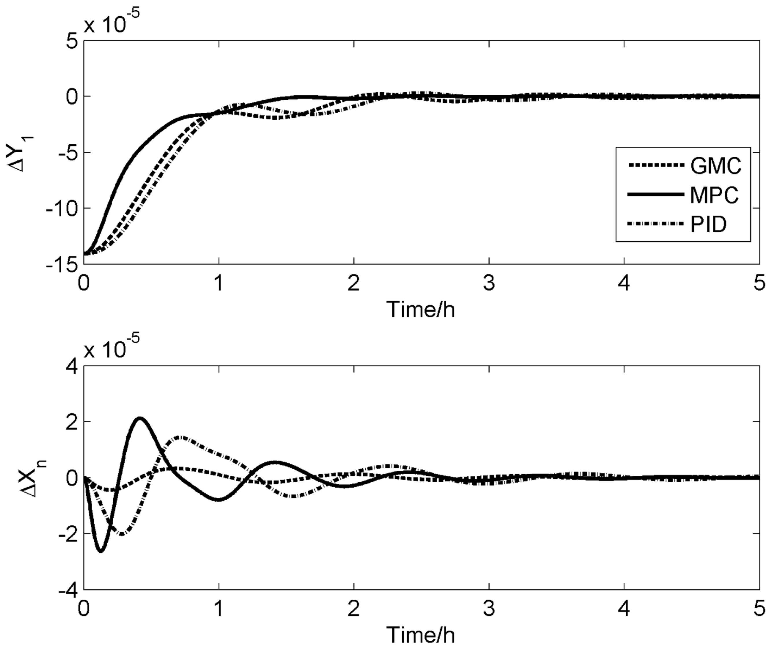
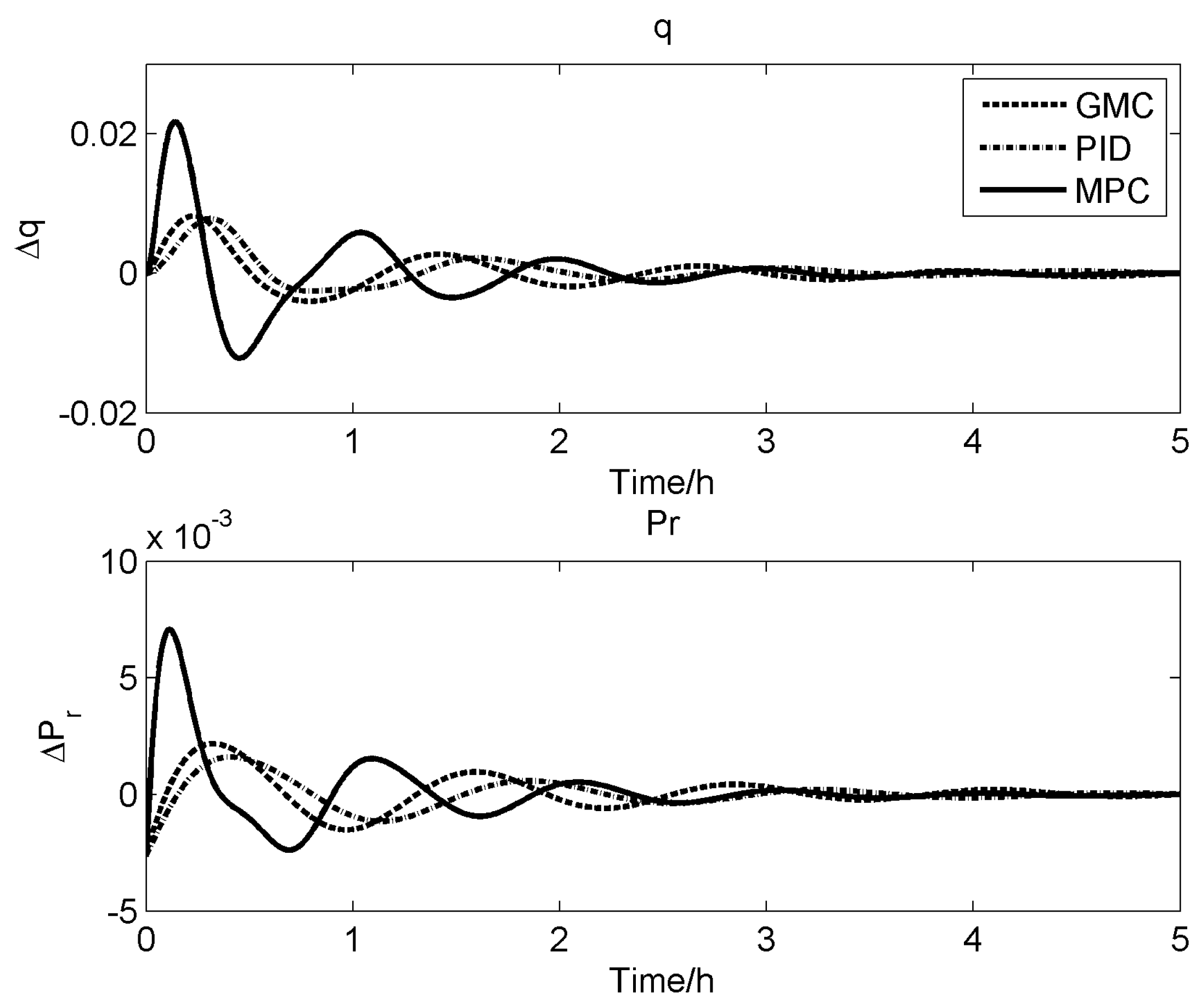
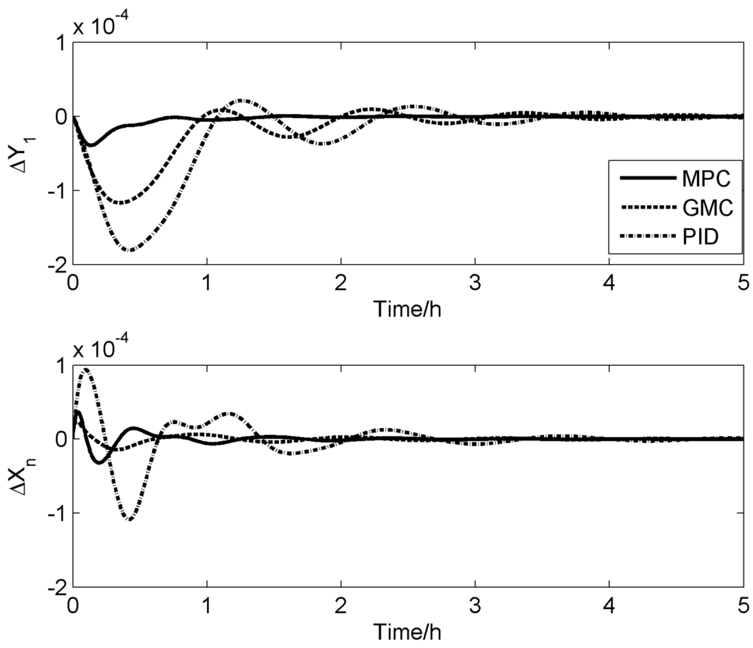
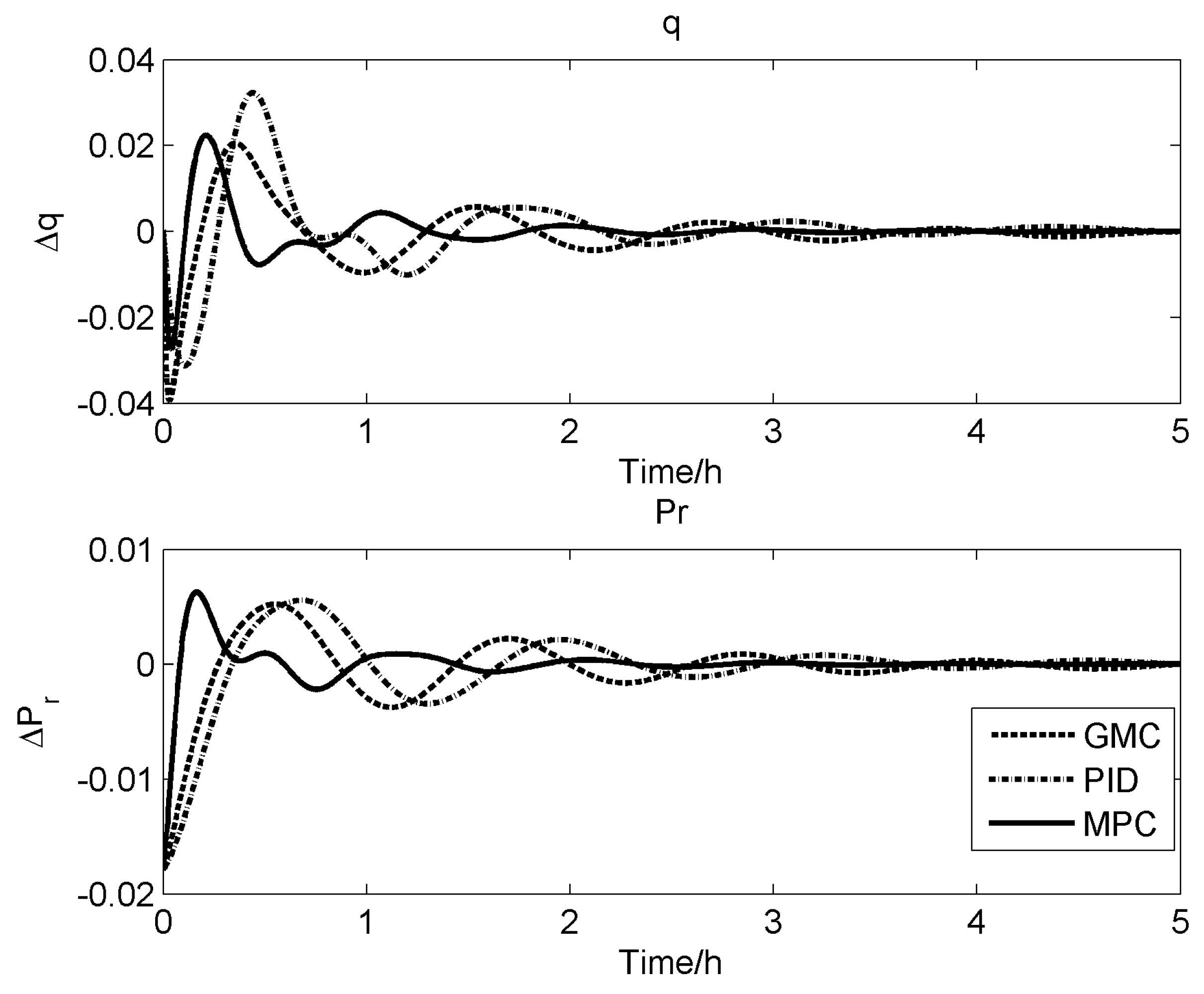
In the forthcoming simulation tests, we compare the control effectiveness of the three control schemes (PID, GMC, MPC) from both the servo control and conventional control viewpoints to observe the variations in control performance among these schemes.

4.1. Servo Control

Figure 7 illustrates the control results of the three control strategies when the setpoint for the top nitrogen concentration is changed from 0.9817 to 0.9819. It can be observed that all three control strategies successfully achieve the control objective. However, since changing setpoints is not commonly encountered in practical processes, this simulation study only serves comparative purposes. From Figure 7, it is evident that MPC exhibits a faster control speed and higher control accuracy. In the rectifying section, MPC enables the nitrogen concentration to reach the new setpoint more rapidly. In the stripping section, despite a slightly larger overshoot, the overall convergence speed is still very rapid in the case of MPC. It might be attributed to the fact that the rectifying section approaches the new setpoint quickly, leading to more intense adjustments of the control variables and consequently resulting in a higher overshoot. Furthermore, as the system approaches near-steady-state conditions, MPC demonstrates less oscillation than PID and GMC, thus achieving a smoother response. In the rectifying section, both GMC and PID show similar control performance. However, in the stripping section, GMC outperforms PID with a smaller overshoot and faster convergence. Figure 8 shows the responses of the control variables for serve control. Apparently, for MPC, the control variables exert a significantly greater influence during the initial stages, leading to a rapid stabilization of the rectifying section but with a relatively larger overshoot in the stripping section. It essentially means that a certain degree of stability is sacrificed for the sake of speed. This trade-off is justified because when the setpoint changes, the primary concern is to bring the product concentration as close to the setpoint as quickly as possible to minimize the production of non-conforming products.

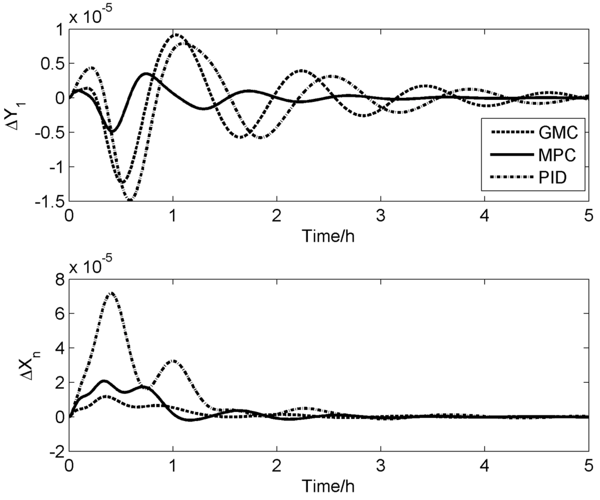
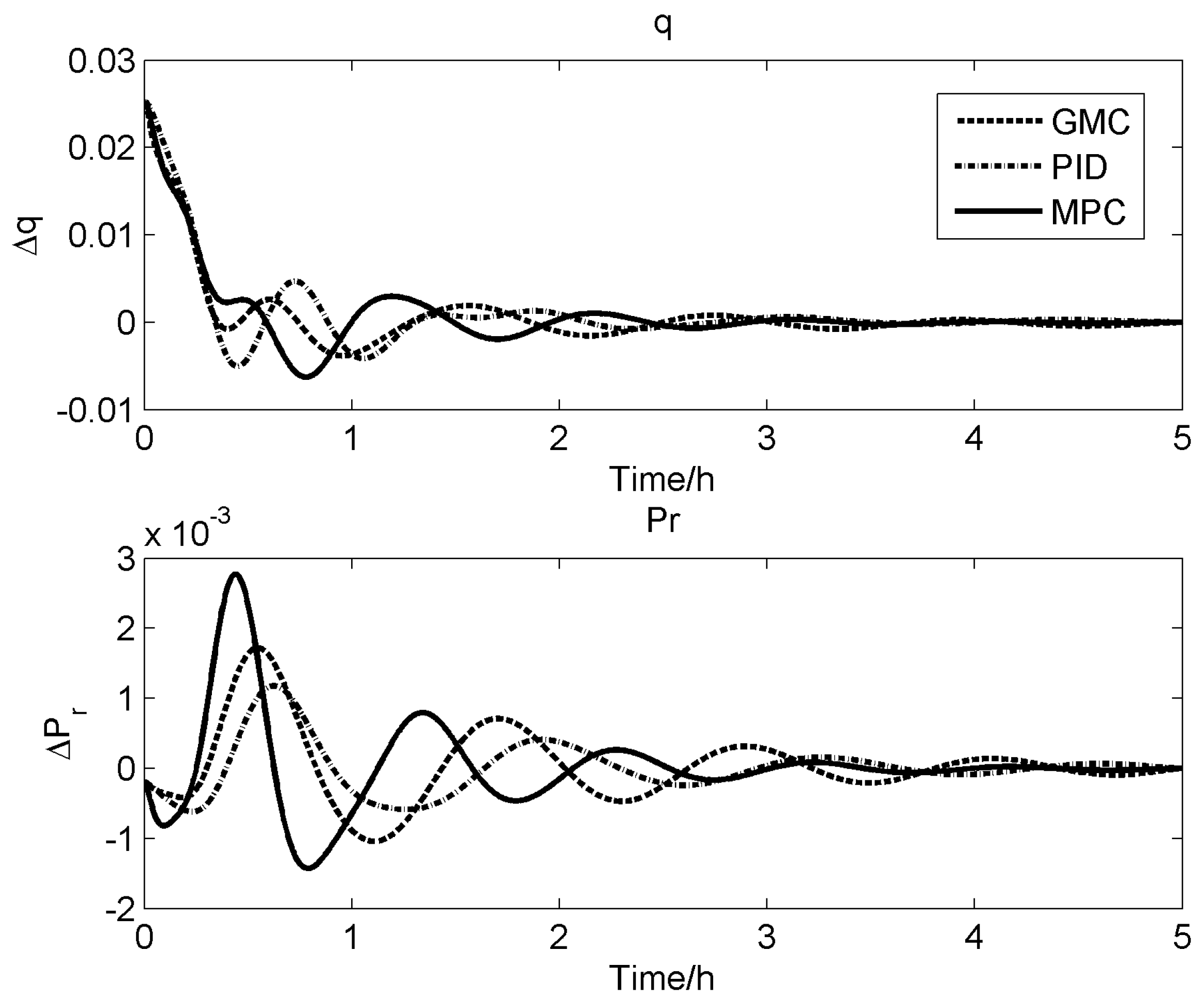
4.2. Regulatory Control

Figure 9 depicts a comparison of the control performance of the three control strategies under a 10% increase in the feed flow rate. When facing the disturbance caused by this change in feed flow rate, the advantages of the MPC approach over the other two control strategies are quite evident. These advantages include a smaller overshoot, faster response time, and better stability. For the GMC and PID control strategies, it is evident that both the rectifying and stripping sections exhibit prolonged oscillations. It indicates that the mutual coupling between these sections poses challenges for the control strategies. In the initial phase of the stripping section, the oscillations in the PID response curve are irregular, implying that the system nonlinearity has a significant impact on the PID control. On the other hand, due to its basis in nonlinear modeling, MPC can adequately capture both the nonlinear and dynamic characteristics of the system. This advantage enables MPC to handle the coupling and nonlinear issues that the other two controllers lack the capability to address. Figure 10 shows the responses of the control variables in this case. From the changes in the control variables, we can also observe that the MPC scheme exhibits a relatively rapid change in control variables at the initial time. In contrast, the other two schemes show a more delayed response, resulting in significant differences in the control performance.
Figure 11 compares the control performance of the three control strategies under a 10% increase in the side stream flow rate. GMC and PID continue to exhibit prolonged oscillations in the rectifying section, while the stability of MPC remains significantly better than the other two methods. In the stripping section, GMC and MPC perform better than PID. It further reveals the relative weakness of PID when dealing with systems characterized by strong nonlinearity. Since the amount of side stream withdrawal is notably smaller than the feed flow rate, the overall fluctuations are considerably smaller than the feed disturbance. Figure 12 shows the responses of the control variables when a 10% increase in the side stream flow rate occurs. Similar to the previous situations, MPC exhibits a more intense response of control variables at the early stage, thus resulting in a faster overall stabilization time.
Comparing Figure 9 and Figure 11, we can observe that the data in Figure 9 is an order of magnitude smaller. It suggests that the system deviation from the original equilibrium state is not as severe, and the established steady-state polynomial model might be a good fit. This improved fit potentially contributes to the better performance of GMC compared to PID. Overall, MPC consistently demonstrates excellent performance in handling both types of disturbances, indicating the effectiveness of the established wave model.

4.3. Error Index Analysis

To enable a more rigorous comparative assessment of the control efficacy exhibited by the controller configurations, we engage in a quantitative appraisal of their performance, using two key performance metrics: the absolute integral error (IAE) and the square integral error (ISE). The mathematical formulations for these quantitative indices are delineated as follows:
I A E = 1 n t k = 1 n t | x ( k ) x * |
I S E = 1 n t k = 1 n t ( x ( k ) x * ) 2
where nt is the total sampling times, x(k) is the controlled variable, and x* corresponds to the set value of the controlled variable.
Table 2, Table 3 and Table 4 provide a comprehensive assessment of the performance metrics for the three control schemes, PID, GMC, and MPC, under three distinct scenarios. It is apparent that GMC and MPC consistently exhibit significantly lower error metrics when contrasted with PID. In the comparison between MPC and GMC, MPC demonstrates a more balanced performance in the two-end control.

5. Conclusions

In this study, a reduced-order HIASC model based on the nonlinear wave theory is proposed to address the challenges faced by the traditional mechanism models in certain online scenarios. The traditional mechanism models involve material balance equations for each tray, resulting in a significant number of differential equations and variables. This complexity makes online solving difficult, especially for model-based control schemes where direct application of the mechanism models can be challenging.
The nonlinear wave model simplifies the model description by treating the concentration profile as a whole and studying its movement and distribution. In this wave model, only two differential equations for the rectifying and stripping sections are needed, eliminating the need for calculations on each tray. Furthermore, due to its mechanism foundation, this model offers higher accuracy than other simplified models, which is beneficial for online model-based control.
Subsequently, we proposed a model predictive control (MPC) strategy based on this model to address the online control problem of HIASC. For comparison purposes, we also employed the PID and GMC control strategies. PID utilized the common dual-loop PI control structure, while GMC was based on a polynomial model identified through data. Through simulation experiments, MPC demonstrated superior control performance compared to the other control strategies in both servo and regulatory control, which further validates the effectiveness of the proposed wave model. Using the wave model in the MPC strategy, the control variables can exhibit a faster response in the initial stages, resulting in an overall better system response.
Note that certain assumptions were made to simplify the derivation, which could introduce model mismatch errors. However, the rolling optimization inherent to MPC helps alleviate these errors. If the model is used for other online estimation tasks, careful consideration of the impact of these errors on the results would be necessary. In the future, further work should focus on establishing more accurate models to address scenarios requiring higher precision results.

Author Contributions

Conceptualization, L.C.; methodology, L.C. and X.L.; software, X.L.; validation, L.C. and X.L.; formal analysis, X.L.; investigation, L.C. and X.L.; writing—original draft preparation, L.C.; writing—review and editing, L.C.; visualization, L.C.; supervision, L.C. All authors have read and agreed to the published version of the manuscript.

Funding

This work was supported by the Natural Science Foundation of Shandong Province, China (Grant ZR2022MB004) and the National Natural Science Foundation of China (Grant 21606255).

Data Availability Statement

Not applicable.

Conflicts of Interest

The authors declare no conflict of interest.

References

  1. Quarshie, A.W.K.; Swartz, C.L.E.; Madabhushi, P.B.; Cao, Y.N.; Wang, Y.J.; Flores-Cerrillo, J. Modeling, simulation, and optimization of multiproduct cryogenic air separation unit startup. AIChE J. 2023, 69, e17953. [Google Scholar] [CrossRef]
  2. Saaedi, M.; Mehrpooya, M.; Delpishe, M.; Zaitsev, A. Proposal and energy/exergy analysis of a novel cryogenic air separation configuration for the production of neon and argon. Chem. Pap. 2022, 76, 7075–7093. [Google Scholar] [CrossRef]
  3. Kong, F.L.; Liu, Y.X.; Tong, L.G.; Guo, W.; Qiu, Y.A.; Wang, L. Optimization of co-production air separation unit based on MILP under multi-product deterministic demand. Appl. Energy 2022, 325, 119850. [Google Scholar] [CrossRef]
  4. Piguave, B.V.; Salas, S.D.; De Cecchis, D.; Romagnoli, J.A. Modular Framework for Simulation-Based Multi-objective Optimization of a Cryogenic Air Separation Unit. ACS Omega 2022, 7, 11696–11709. [Google Scholar] [CrossRef]
  5. Huo, C.; Sun, J.; Song, P. Energy, exergy and economic analyses of an optimal use of cryogenic liquid turbine expander in air separation units. Chem. Eng. Res. Des. 2023, 189, 194–209. [Google Scholar] [CrossRef]
  6. Maroukis, G.; Georgiadis, M.C. Modeling, simulation, and techno-economic optimization of argon separation processes. Chem. Eng. Res. Des. 2022, 184, 165–179. [Google Scholar] [CrossRef]
  7. Kender, R.; Roessler, F.; Wunderlich, B.; Pottmann, M.; Thomas, I.; Ecker, A.-M.; Rehfeldt, S.; Klein, H. Improving the load flexibility of industrial air separation units using a pressure-driven digital twin. AlChE J. 2022, 68, e17692. [Google Scholar] [CrossRef]
  8. Saedi, M.; Mehrpooya, M.; Shabani, A.; Zaitsev, A.; Nikitin, A. Proposal and investigation of a novel process configuration for production of neon from cryogenic air separation unit. Sustain. Energy Technol. Assess. 2022, 50, 101875. [Google Scholar] [CrossRef]
  9. Cheng, M.; Verma, P.; Yang, Z.W.; Axelbaum, R.L. Flexible cryogenic air separation unit-An application for low-carbon fossil-fuel plants. Sep. Purif. Technol. 2022, 302, 122086. [Google Scholar] [CrossRef]
  10. Chang, L.; Liu, X.G. Sidestream Analysis and Optimization of Full Tower Internal Thermally Coupled Air Separation Columns. Chem. Eng. Technol. 2014, 37, 667–674. [Google Scholar] [CrossRef]
  11. Jana, A.K. Heat integrated distillation operation. Appl. Energ. 2010, 87, 1477–1494. [Google Scholar] [CrossRef]
  12. Jana, A.K. Performance analysis of a heat integrated column with heat pumping. Sep. Purif. Technol. 2019, 209, 18–25. [Google Scholar] [CrossRef]
  13. Duan, W.T.; Yang, M.B.; Feng, X. Comprehensive Analysis and Targeting of Distillation Integrated into Overall Process Considering Operating Pressure Change. Processes 2022, 10, 1861. [Google Scholar] [CrossRef]
  14. Aurangzeb, M.; Jana, A.K. A Novel Heat Integrated Extractive Dividing Wall Column for Ethanol Dehydration. Ind. Eng. Chem. Res. 2019, 58, 9109–9117. [Google Scholar] [CrossRef]
  15. Liu, C.; Yang, D.; Zhang, Q.; Zhang, Q.; Cui, C. Control of fully heat-integrated pressure-swing distillation with strict pressure manipulation: A case study of separating a maximum-boiling azeotrope with small pressure-induced shift. Sep. Purif. Technol. 2023, 323, 124455. [Google Scholar] [CrossRef]
  16. Yuan, H.; Luo, Y.; Yuan, X. Synthesis of heat-integrated distillation sequences with mechanical vapor recompression by stochastic optimization. Comput. Chem. Eng. 2022, 165, 107922. [Google Scholar] [CrossRef]
  17. Gu, J.; Lu, S.; Shi, F.; Wang, X.; You, X. Economic and Environmental Evaluation of Heat-Integrated Pressure-Swing Distillation by Multiobjective Optimization. Ind. Eng. Chem. Res. 2022, 61, 9004–9014. [Google Scholar] [CrossRef]
  18. Li, Y.; Jiang, Y.; Xu, C. Robust Control of Partially Heat-Integrated Pressure-Swing Distillation for Separating Binary Maximum-Boiling Azeotropes. Ind. Eng. Chem. Res. 2019, 58, 2296–2309. [Google Scholar] [CrossRef]
  19. Chen, Y.; Liu, C.; Geng, Z. Design and control of fully heat-integrated pressure swing distillation with a side withdrawal for separating the methanol/methyl acetate/acetaldehyde ternary mixture. Chem. Eng. Process. 2018, 123, 233–248. [Google Scholar] [CrossRef]
  20. Cao, Y.; Swartz, C.L.E.; Flores-Cerrillo, J.; Ma, J. Dynamic Modeling and Collocation-Based Model Reduction of Cryogenic Air Separation Units. AlChE J. 2016, 62, 1602–1615. [Google Scholar] [CrossRef]
  21. Van der Ham, L.V. Improving the exergy efficiency of a cryogenic air separation unit as part of an integrated gasification combined cycle. Energy Convers. Manag. 2012, 61, 31–42. [Google Scholar] [CrossRef]
  22. Van der Ham, L.V.; Kjelstrup, S. Improving the Heat Integration of Distillation Columns in a Cryogenic Air Separation Unit. Ind. Eng. Chem. Res. 2011, 50, 9324–9338. [Google Scholar] [CrossRef]
  23. Fu, Y.; Liu, X. Nonlinear dynamic behaviors and control based on simulation of high-purity heat integrated air separation column. ISA Trans. 2015, 55, 145–153. [Google Scholar] [CrossRef]
  24. Zhang, P.K.; Liang, J.Y.; Yang, Y.H.; Wang, L. A new heating system for the air pre-purification of air separation units. Appl. Therm. Eng. 2023, 226, 120194. [Google Scholar] [CrossRef]
  25. Mora, C.A.; Orjuela, A. Modeling, validation and exergy evaluation of a thermally-integrated industrial cryogenic air separation plant in Colombia. Chem. Eng. Res. Des. 2022, 185, 73–86. [Google Scholar] [CrossRef]
  26. Wang, Z.; Qin, W.; Yang, C.; Wang, W.; Xu, S.; Gui, W.; Sun, Y.; Xie, D.; Wang, Y.; Lu, J.; et al. Heat-transfer distribution optimization for the heat-integrated air separation column. Sep. Purif. Technol. 2020, 248, 117048. [Google Scholar] [CrossRef]
  27. Jaleel, E.A.; Anzar, S.M.; Beegum, T.R.; Shahid, P.A.M. System identification and control of heat integrated distillation column using artificial bee colony based support vector regression. Chem. Eng. Commun. 2022, 209, 1377–1396. [Google Scholar] [CrossRef]
  28. Jaleel, E.A.; Anzar, S.M.; Koya, A.M. Machine learning based system identification of a realistic heat integrated distillation column using particle swarm optimization. Chem. Eng. Commun. 2023, 210, 1694–1714. [Google Scholar] [CrossRef]
  29. Cong, L.; Liu, X. Nonlinear-Model-Based Control of a Heat Integrated Distillation Column Using Model Updating Based on Distributed Wave Velocity. Ind. Eng. Chem. Res. 2019, 58, 20758–20768. [Google Scholar] [CrossRef]
  30. Tan, H.Y.; Cong, L. Modeling and Control Design for Distillation Columns Based on the Equilibrium Theory. Processes 2023, 11, 607. [Google Scholar] [CrossRef]
  31. Luyben, W.L. Profile Position Control of Distillation Columns with Sharp Temperature Profiles. AIChE J. 1972, 18, 238–240. [Google Scholar] [CrossRef]
  32. Luyben, W.L. Control of heat-integrated extractive distillation processes. Comput. Chem. Eng. 2018, 111, 267–277. [Google Scholar] [CrossRef]
  33. Luyben, W.L. Control of Distillation Columns with Sharp Temperature Profiles. AIChE J. 1971, 17, 713–718. [Google Scholar] [CrossRef]
  34. Kim, B.-k.; Hwang, H.; Woo, D.; Han, M. Design and Control of a Reactive Distillation Column Based on a Nonlinear Wave Propagation Theory: Production of Terephthalic Acid. Ind. Eng. Chem. Res. 2010, 49, 4297–4307. [Google Scholar] [CrossRef]
  35. Hwang, Y.L.; Graham, G.K.; Keller, G.E.; Ting, J.; Helfferich, F.G. Experimental study of wave propagation dynamics of binary distillation columns. AIChE J. 1996, 42, 2743–2760. [Google Scholar] [CrossRef]
  36. Hwang, Y.L. On the Nonlinear-Wave Theory for Dynamics of Binary Distillation-Columns. AIChE J. 1995, 41, 190–194. [Google Scholar] [CrossRef]
  37. Hwang, Y.L. Nonlinear-Wave Theory for Dynamics of Binary Distillation-Columns. AIChE J. 1991, 37, 705–723. [Google Scholar] [CrossRef]
  38. Hwang, Y.L.; Helfferich, F.G. Nonlinear-Waves and Asymmetric Dynamics of Countercurrent Separation Processes. AIChE J. 1989, 35, 690–693. [Google Scholar] [CrossRef]
  39. Cong, L.; Xu, L.Q.; Liu, X.G. Adaptive Temperature Control for Distillation Columns Based on Relative Stability in the Profile Pattern. Ind. Eng. Chem. Res. 2021, 60, 514–527. [Google Scholar] [CrossRef]
  40. Cong, L.; Liu, X.; Deng, X.; Chen, H. Development of a partially accurate model and application to a reduced-order control scheme for heat integrated distillation column. Sep. Purif. Technol. 2019, 229, 115809. [Google Scholar] [CrossRef]
  41. Cheng, Y.; Chen, Z.Q.; Sun, M.W.; Sun, Q.L. Decoupling control of high-purity heat integrated distillation column process via active disturbance rejection control and nonlinear wave theory. Trans. Inst. Meas. Control. 2020, 42, 2221–2233. [Google Scholar] [CrossRef]
  42. Cong, L.; Liu, X. Temperature Inferential Control of Heat-Integrated Distillation Column Based on Variable Sensitive Stage Temperature Set-point. Can. J. Chem. Eng. 2019, 97, 2952–2960. [Google Scholar] [CrossRef]
  43. Peng, D.-Y.; Robinson, D.B. A new two constant equation of state. Ind. Eng. Chem. Fundam. 1976, 15, 59–64. [Google Scholar] [CrossRef]
Figure 1. Schematic diagram of the HIASC. (Reproduced with permission from Lin Cong et al., Chemical Engineering and Technology; published by John Wiley and Sons, 2018).
Processes 11 02918 g001
Figure 2. Schematic diagram of concentration wave propagation.
Processes 11 02918 g002
Figure 3. Simplified schematic diagram of wave propagation.
Processes 11 02918 g003
Figure 4. Variation in wave velocity for the rectifying column and stripping column.
Processes 11 02918 g004
Figure 5. Dynamic tracking of nitrogen product concentration at the column top.
Processes 11 02918 g005
Figure 6. Dynamic tracking of oxygen product concentration at the column bottom.
Processes 11 02918 g006
Figure 7. Comparison of servo control effects.
Processes 11 02918 g007
Figure 8. Responses of the control variables in servo control.
Processes 11 02918 g008
Figure 9. Comparison of control performance with a 10% increase in feed flow rate.
Processes 11 02918 g009
Figure 10. Responses of the control variables with a 10% increase in feed flow rate.
Processes 11 02918 g010
Figure 11. Comparison of control performance with a 10% increase in side stream flow rate.
Processes 11 02918 g011
Figure 12. Responses of the control variables with a 10% increase in side stream flow rate.
Processes 11 02918 g012
Table 1. The operating conditions of the HIASC.
Operating ConditionValueOperating ConditionValue
Flow rate F (kmol/s)10Feed composition (O2)0.2095
Feed temperature Tf (K)102.2Feed composition (N2)0.7812
Feed stage20Pressure of the rectifying column (MPa)0.69
Stage number40Pressure of the stripping column (MPa)0.13
Feed thermal condition0.696Nitrogen product purity0.9817
Side stream stage26Oxygen product purity0.9929
Side stream flow rate (kmol/s)0.08
Table 2. Error index of PID.
Servo ControlF + 10%Sf + 10%
IAE_Y11.98 × 10−53.06 × 10−52.93 × 10−6
IAE_Xn3.78 × 10−61.51 × 10−59.47 × 10−6
ISE_Y11.76 × 10−93.39 × 10−91.89 × 10−11
ISE_Xn3.63 × 10−117.68 × 10−103.64 × 10⁻¹⁰
Table 3. Error index of GMC.
Servo ControlF + 10%Sf + 10%
IAE_Y11.85 × 10−51.88 × 10−52.69 × 10−6
IAE_Xn8.93 × 10−72.43 × 10−61.84 × 10−6
ISE_Y11.54 × 10−91.34 × 10−91.56 × 10−11
ISE_Xn1.77 × 10−121.89 × 10−111.18 × 10⁻¹¹
Table 4. Error index of MPC.
Servo ControlF + 10%Sf + 10%
IAE_Y11.18 × 10−53.00 × 10−66.63 × 10−7
IAE_Xn3.16 × 10−62.87 × 10−63.26 × 10−6
ISE_Y19.06 × 10−106.18 × 10−111.49 × 10⁻¹²
ISE_Xn3.84 × 10−114.67× 10−114.30 × 10⁻¹¹
Disclaimer/Publisher’s Note: The statements, opinions and data contained in all publications are solely those of the individual author(s) and contributor(s) and not of MDPI and/or the editor(s). MDPI and/or the editor(s) disclaim responsibility for any injury to people or property resulting from any ideas, methods, instructions or products referred to in the content.

