

A Data-Driven Approach for the Ultra-Supercritical Boiler Combustion Optimization Considering Ambient Temperature Variation: A Case Study in China
Abstract
:1. Introduction
- We quantitatively analyzed the impact of AT changes on boiler combustion control and used the fuzzy C-means (FCM) clustering algorithm to use the AT as the basis for working conditions to improve the accuracy of the linear model;
- Subdivide the complex non-linear operating conditions of the boiler into simple operating conditions that can be linearly processed. Aiming at the industrial production data of coal-fired boilers in the Weifang Power Plant, an MLR model is used to establish the mapping relationship between manipulated variables and boiler efficiency, and the model is suitable for online application;
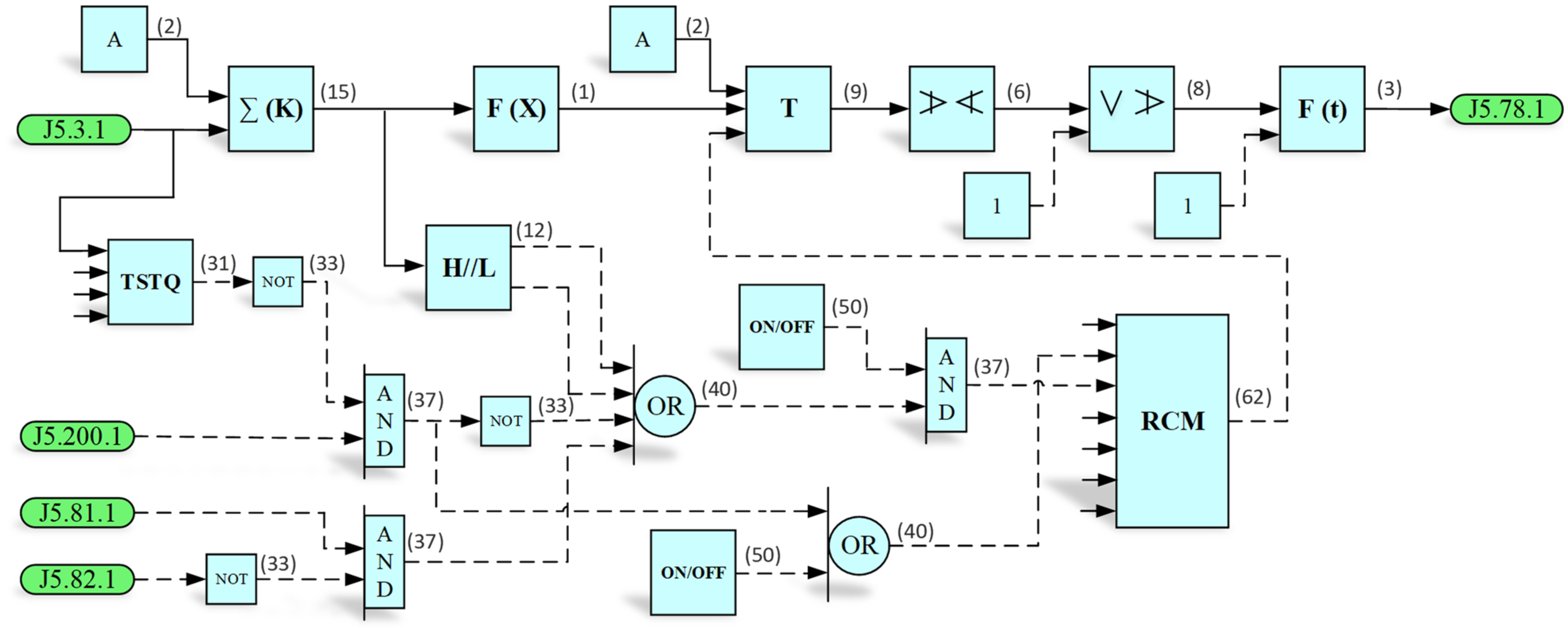
- Using partial differential derivation to calculate the optimal control deviation of model variables and participating in the boiler online real-time closed-loop control by embedding the DCS configuration logic is a practical attempt under carbon neutrality.
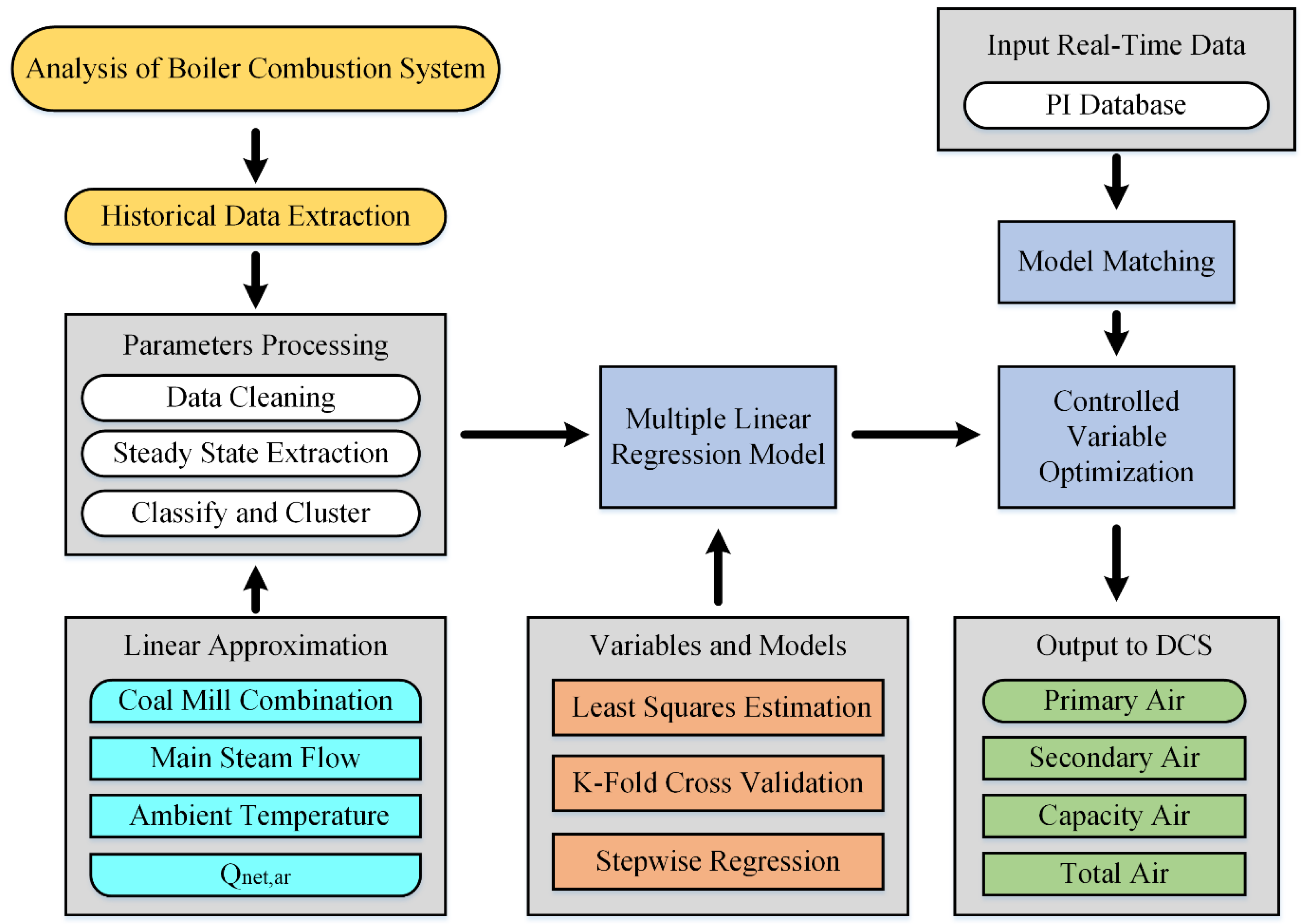
2. Analysis of the Boiler Combustion System
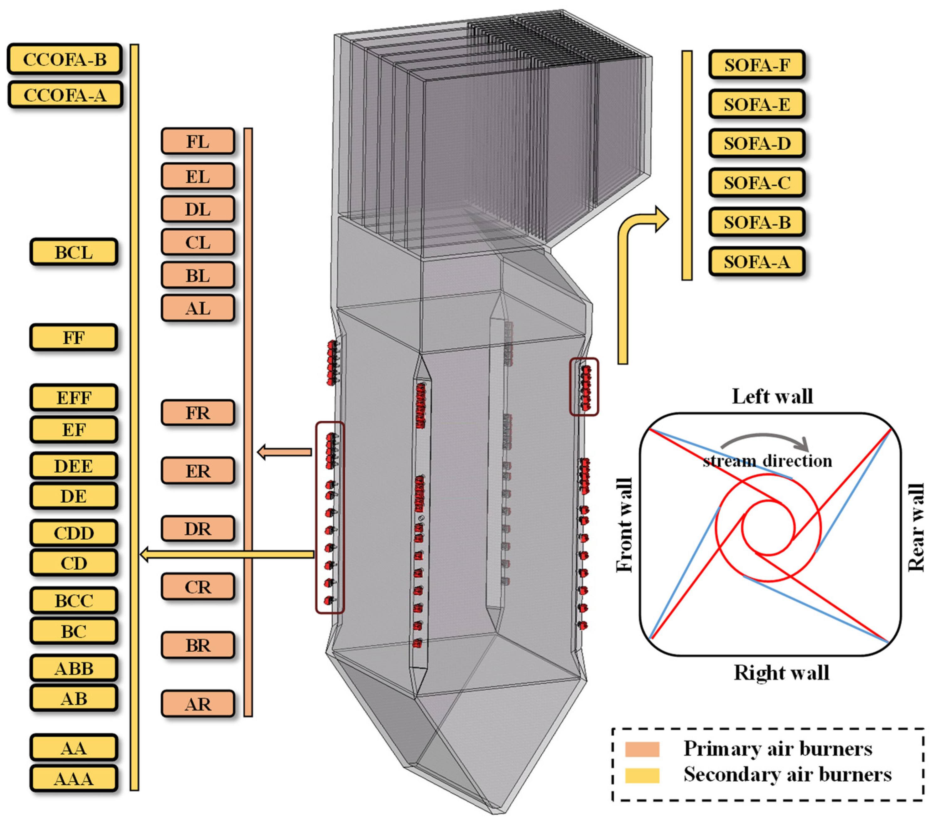
2.1. Description of the Boiler Combustion System
2.2. Variable Analysis and Selection
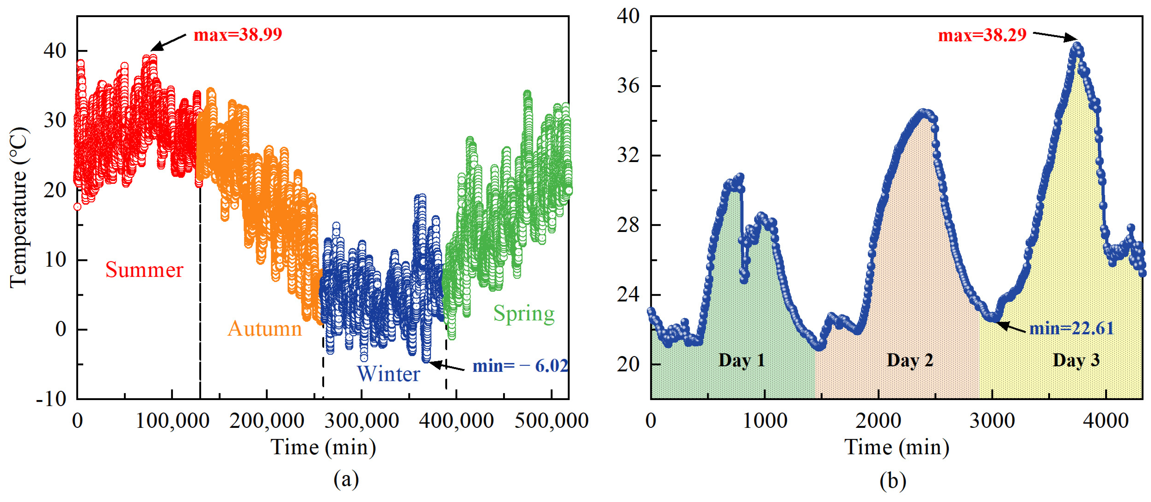
2.2.1. The Influence of AT on the Total Air Flow of the Boiler
2.2.2. The Influence of COM-Mill on Damper Control
2.2.3. Variable Selection
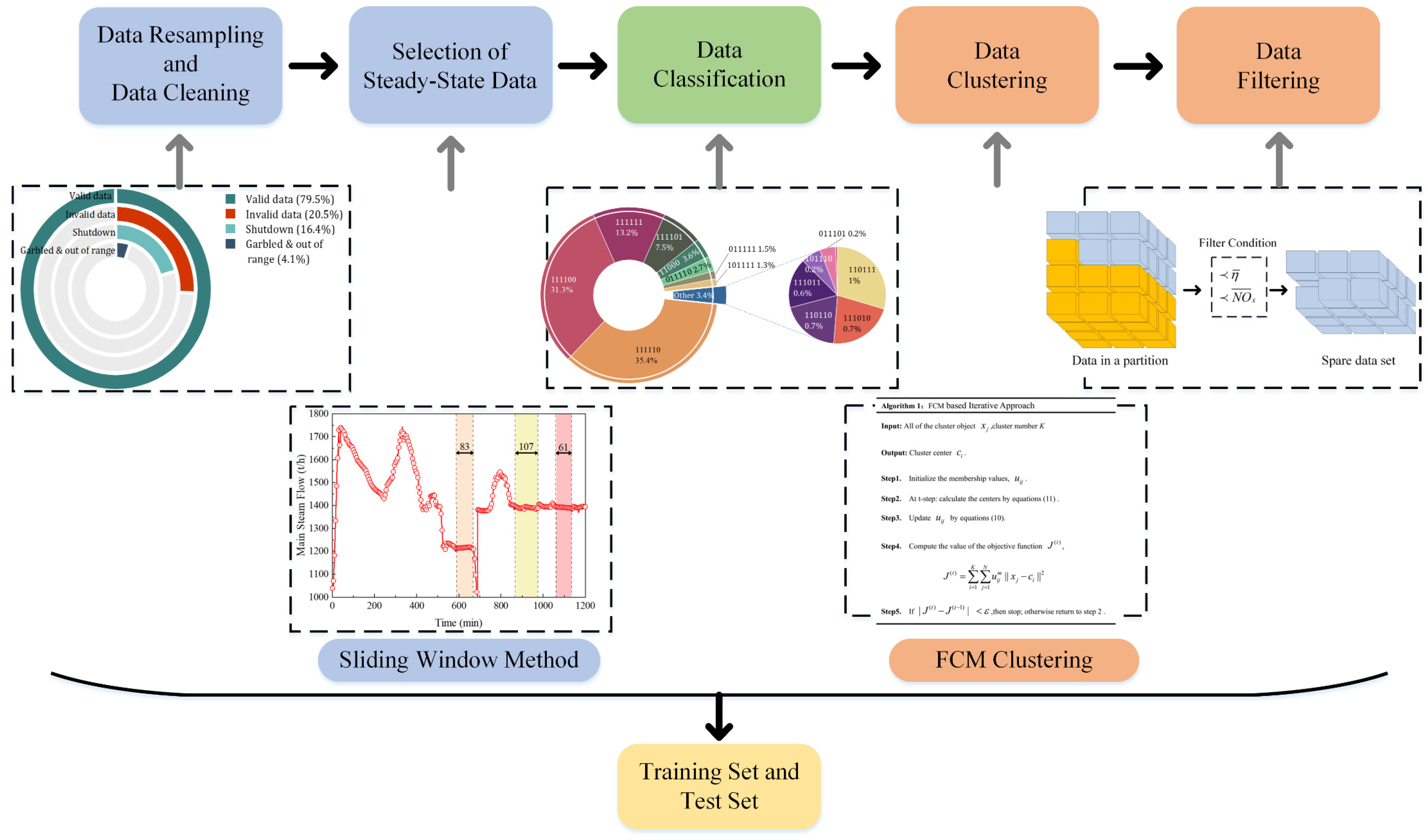
3. Data Processing
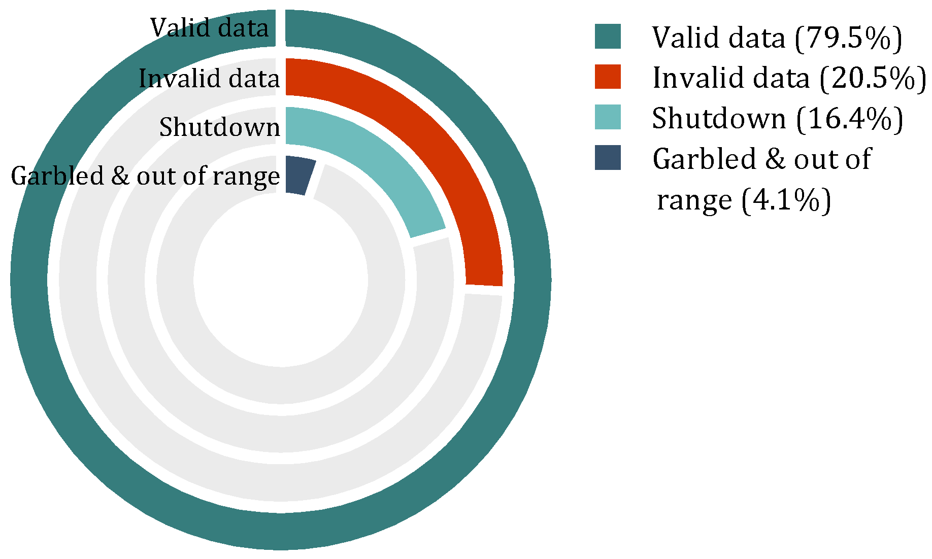
3.1. Data Cleaning
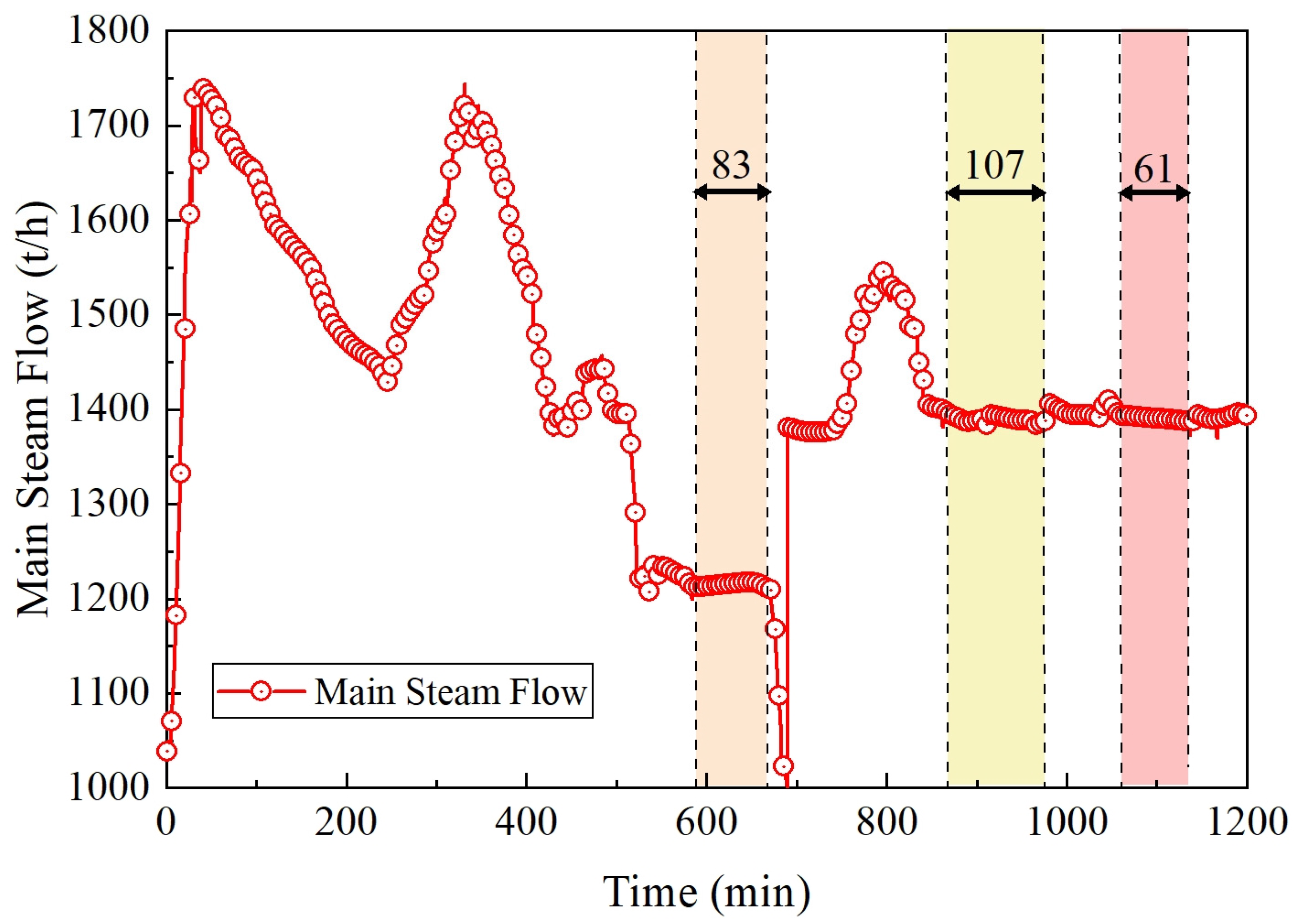
3.2. Selection of Steady-State Data
3.3. Cluster Analysis
3.3.1. Data Classification
3.3.2. Clustering Method
| Algorithm 1: FCM-based Iterative Approach |
| Input: , cluster number K |
| Output: |
| Step1. |
| Step2. At t-step: calculate the centers by Equation (8). |
| Step3. by Equation (9). |
| Step4., |
| Step5., then stop; otherwise return to step 2. |
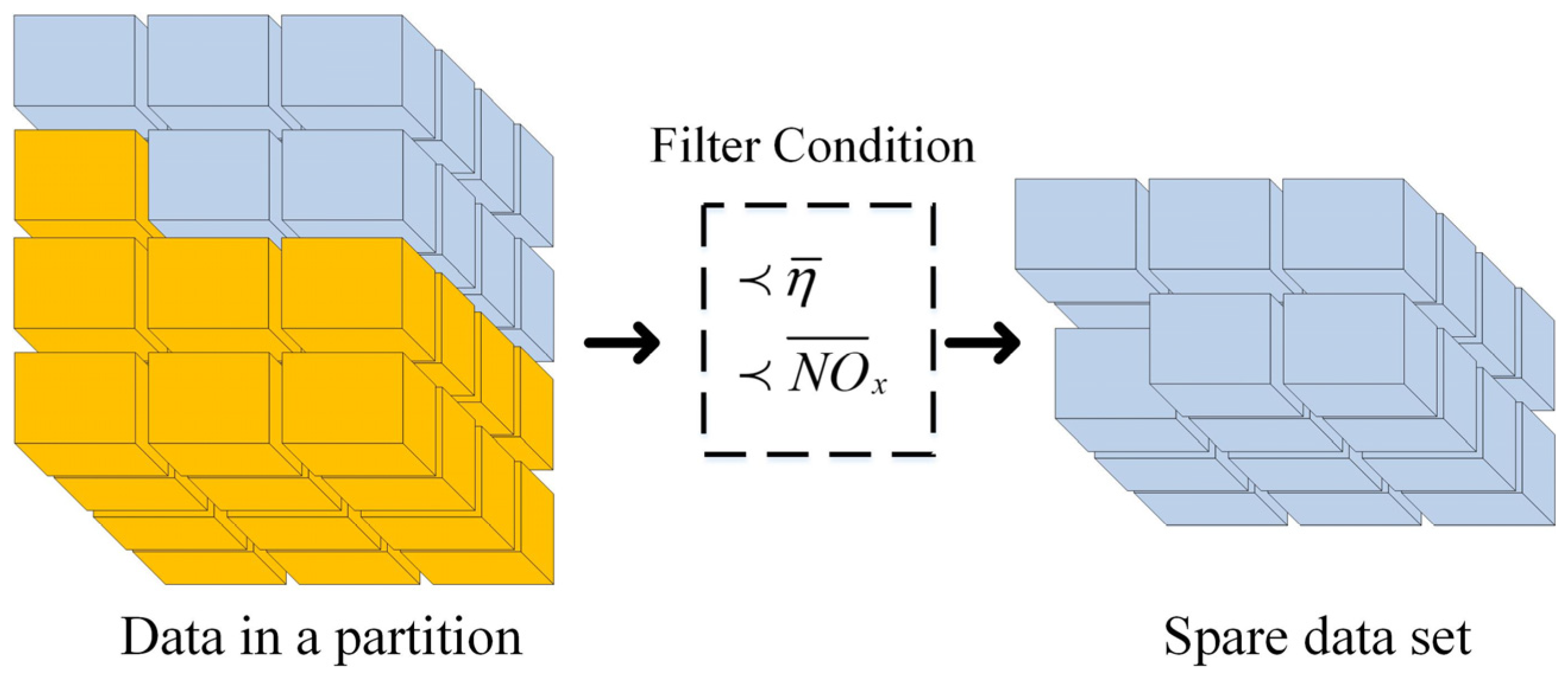
3.4. Data Filtering
3.5. A Case Study
4. MLR Model
4.1. Model Description
4.2. Least Squares Estimation of Regression Parameters
4.3. Optimal Model Selection
4.3.1. SRM to Determine the Regression Variable
4.3.2. Model Performance Criterion
4.4. Optimization of Manipulated Variables
5. Test Analysis and Industrial Online Application
5.1. Application Test Analysis
5.1.1. Selection of Historical Data
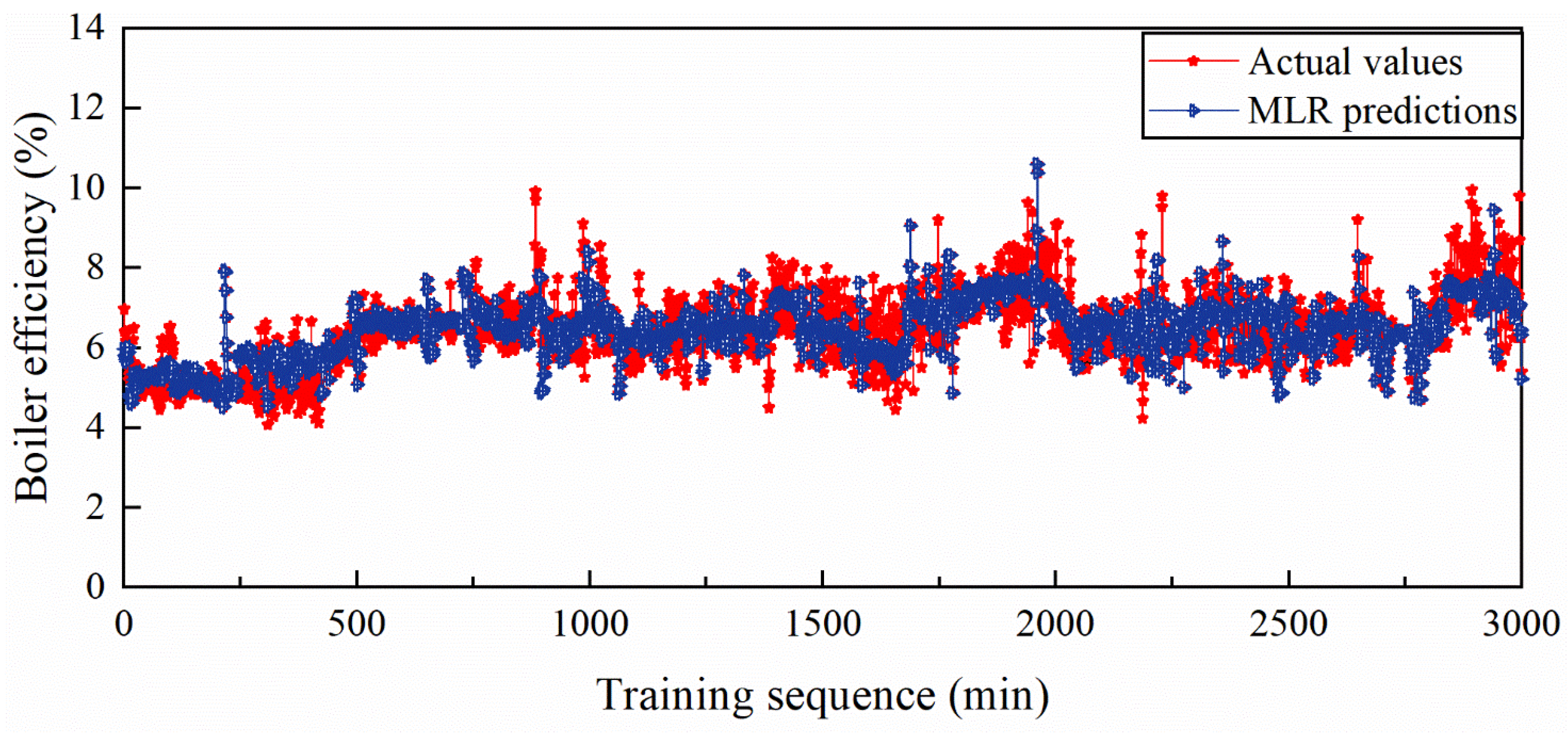
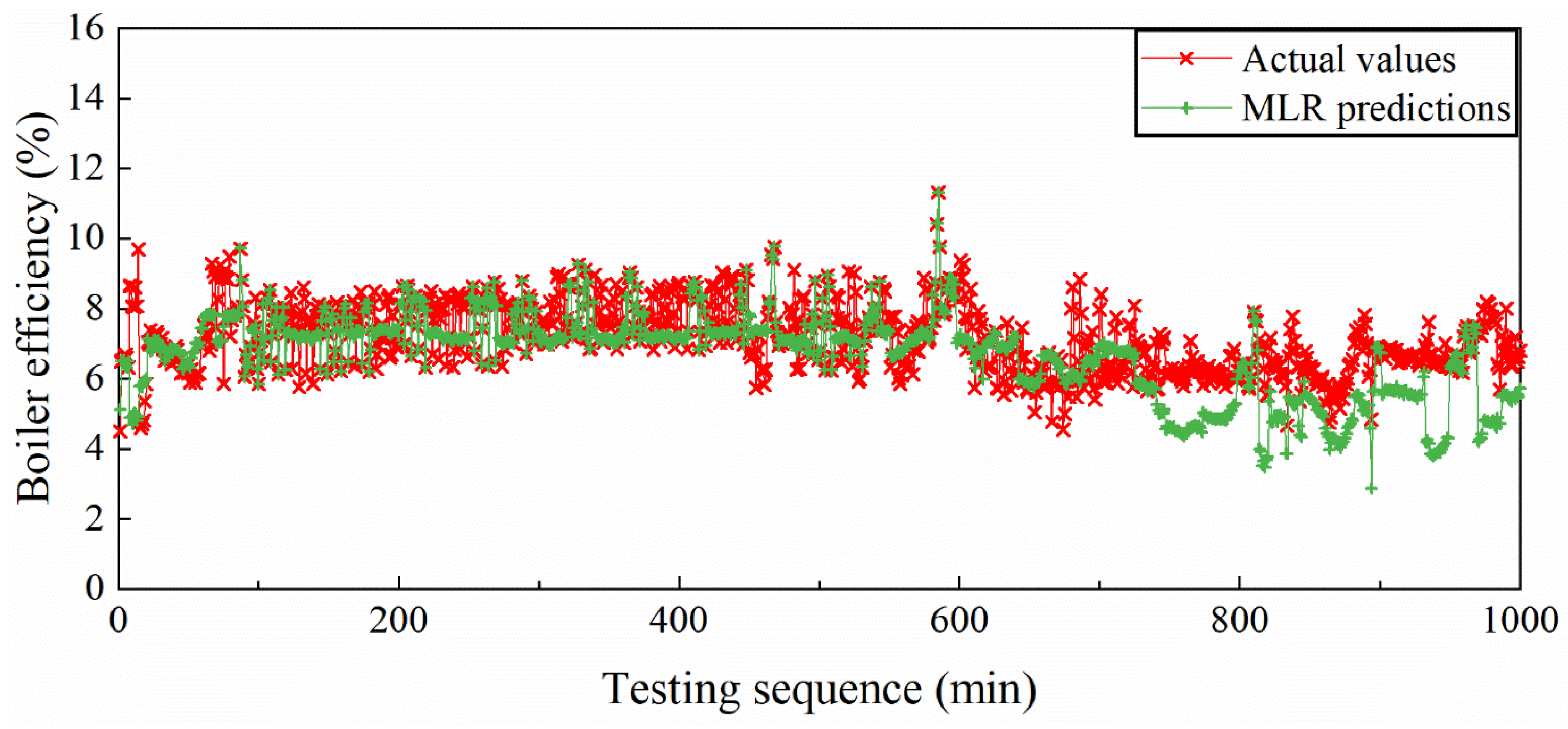
5.1.2. MLR Model and Prediction Performance
5.2. Online Test of Combustion Optimization System
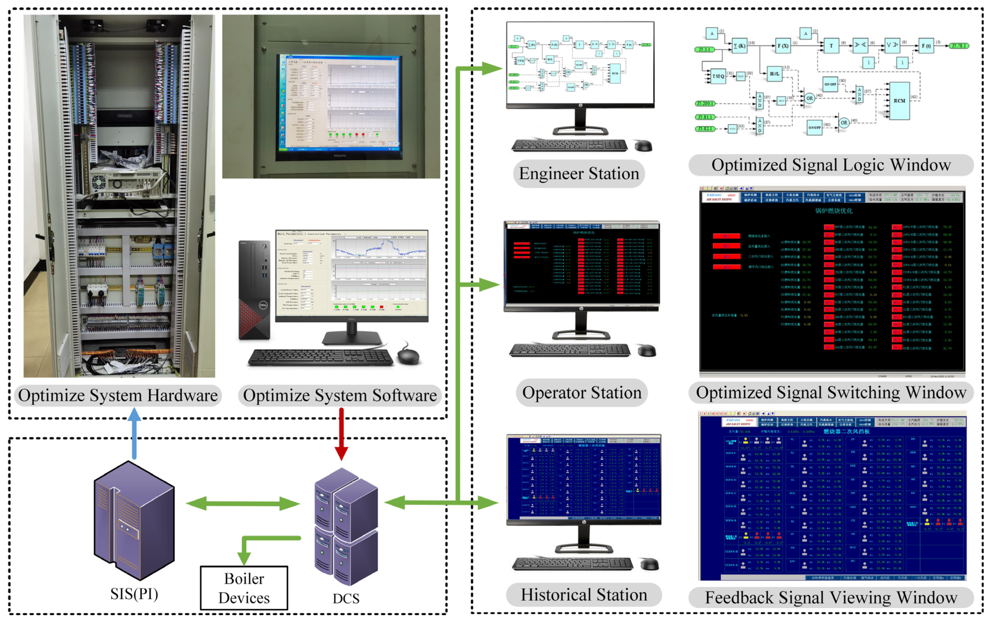
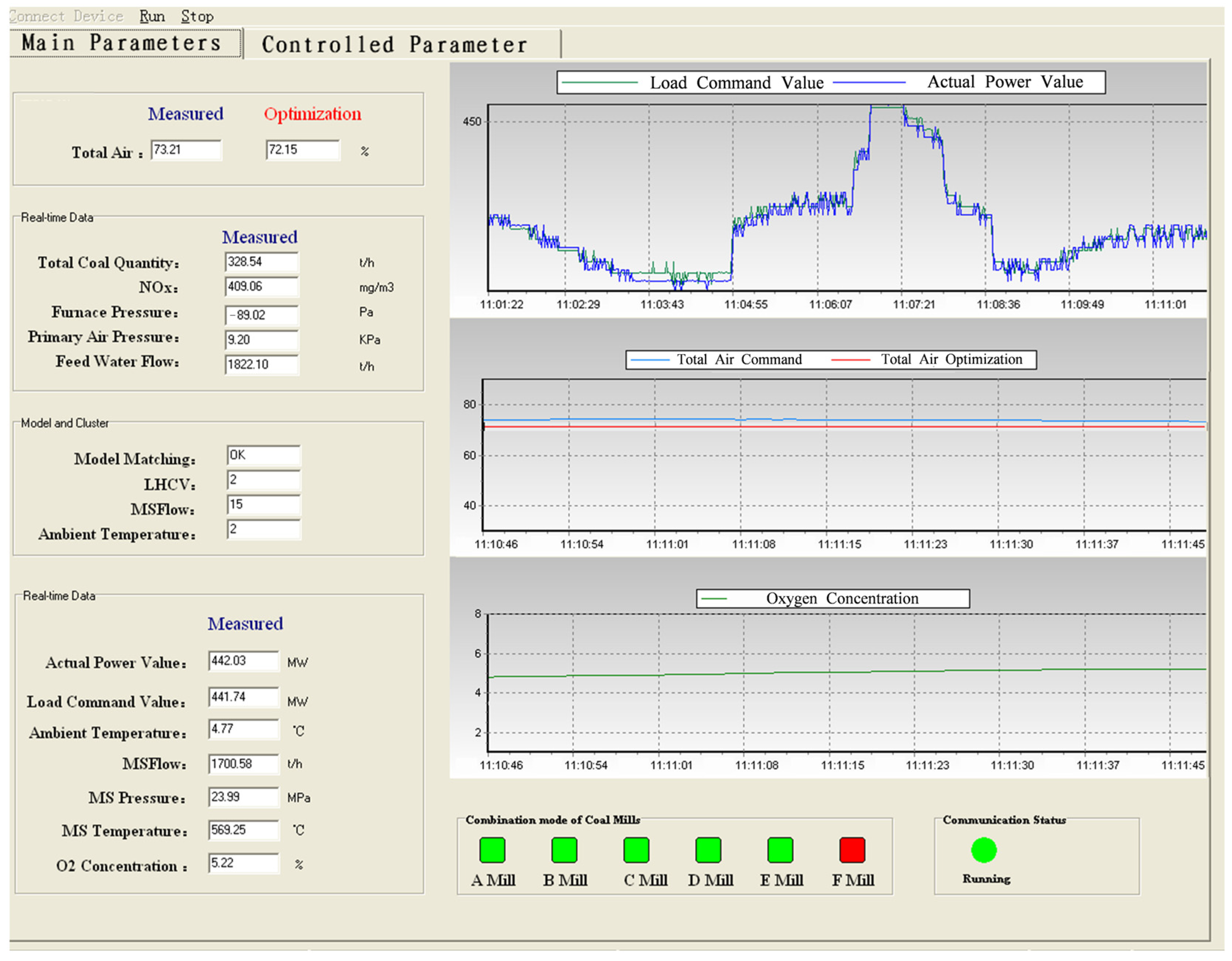
5.2.1. System Description
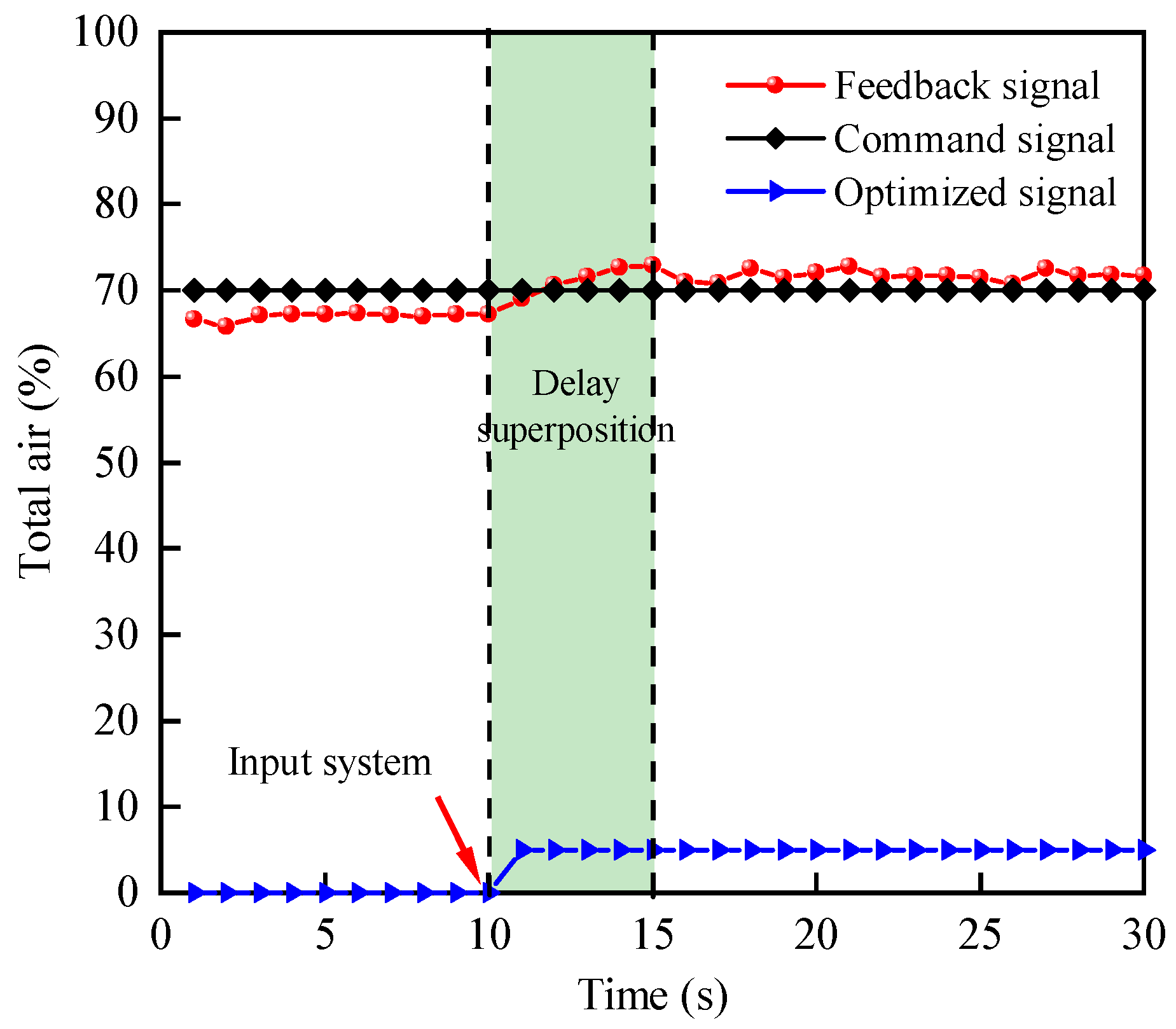
5.2.2. Full-Scale Test
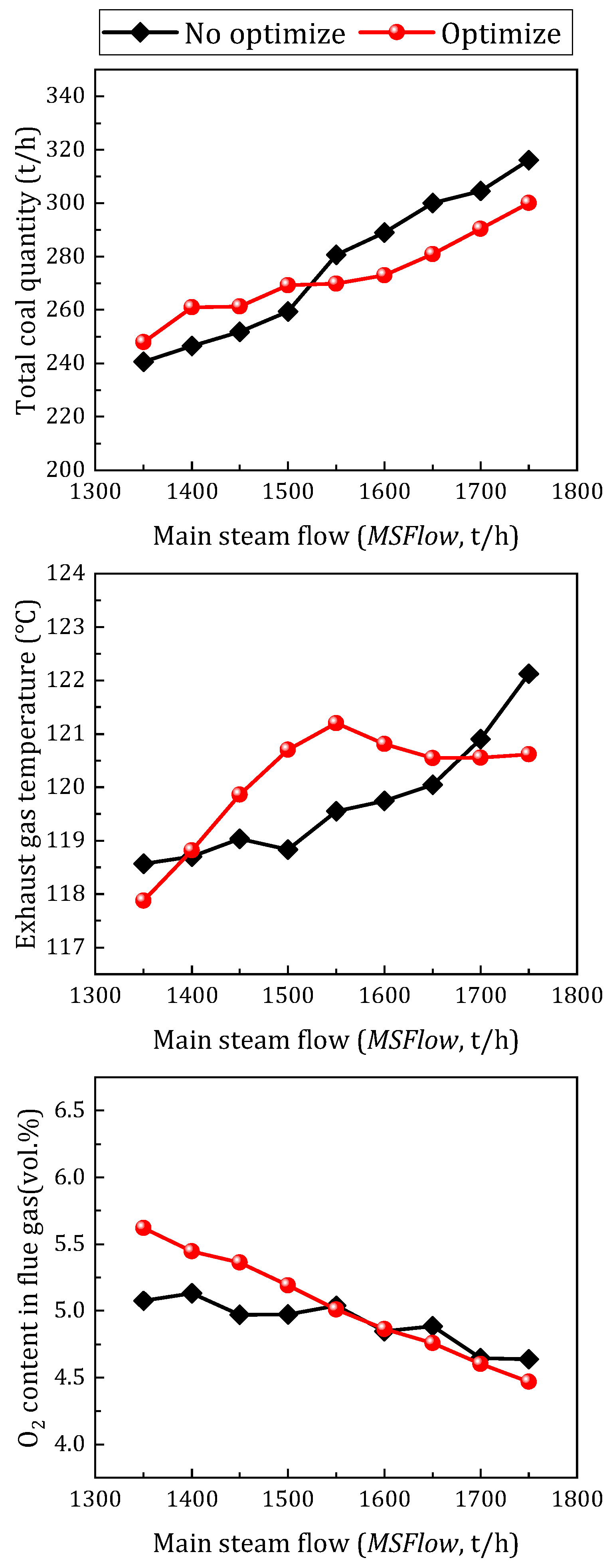
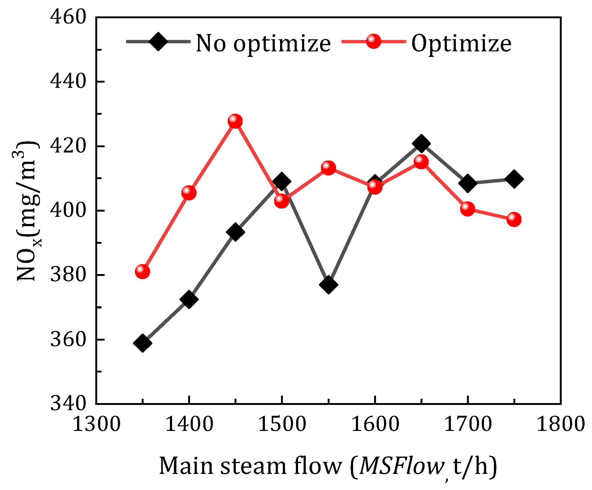
5.2.3. Analysis of the Test Results
6. Conclusions
Author Contributions
Funding
Institutional Review Board Statement
Informed Consent Statement
Data Availability Statement
Conflicts of Interest
Nomenclature
| Acronyms | |
| DCS | Distributed Control System |
| SIS | Supervisory Information System |
| PI | Plant Information System |
| CFD | Computational Fluid Dynamic |
| ANN | Artificial Neural Network |
| GA | Genetic Algorithm |
| SVR | Support Vector Regression |
| MLR | Multiple Linear Regression |
| CCS | Carbon Capture and Storage |
| MSF | Main Steam Flow |
| AT | Ambient Temperature |
| LHVC | Lower Heating Value of Coal |
| SRA | Stepwise Regression Algorithm |
| FCM | Fuzzy C-Means |
| CV | Controlled Variable |
| MV | Manipulated Variable |
| OCS | Online Control System |
| LNCFS | Low NOx Concentric Firing System |
| SOFA | Separated Over Fire Air |
| CCOFA | Close-Coupled Over Fire Air |
| UFA | Underfire Air |
| MCR | Maximum Continuous Rating |
| BMCR | Boiler Maximum Continuous Rating |
| SCR | Selective Catalytic Reduction |
| RMSE | Root Mean Square Error |
| I/O | Input/Output |
| SQL | Structured Query Language |
| Symbols | |
| Defined boiler efficiency | |
| J(t) | The value of the objective function after the iteration |
| ε | Convergence condition of objective function iteration |
| The significance level of the introduced variable | |
| The significance level of the eliminated variable | |
References
- Nakaishi, T. Developing effective CO2 and SO2 mitigation strategy based on marginal abatement costs of coal-fired power plants in China. Appl. Energy 2021, 294, 116978. [Google Scholar] [CrossRef]
- United Nations. Statement by H.E. Xi Jinping President of the People’s Republic of China at the General Debate of the 75th Session of the United Nations General 2020. Assembly 2020; Ministry of Foreign Affairs of the People’s Republic of China: Beijing, China, 2020. [Google Scholar]
- Shan, Y.; Guan, D.; Zheng, H.; Ou, J.; Li, Y.; Meng, J.; Mi, Z.; Liu, Z.; Zhang, Q. China CO2 emission accounts 1997–2015. Sci. Data 2018, 5, 170201. [Google Scholar] [CrossRef] [PubMed]
- The Central People’s Government of the People’s Republic of China. Xi Jinping: China Promises to Achieve the Time from Carbon Peak to Carbon Neutralization, Much Shorter than the Time Spent in Developed Countries. 2021. Available online: http://www.gov.cn/xinwen/2021-04/22/content_5601515.htm (accessed on 6 August 2021). (In Chinese)
- Milićević, A.; Belošević, S.; Crnomarković, N.; Tomanović, I.; Tucaković, D. Mathematical modelling and optimization of lignite and wheat straw co-combustion in 350 MWe boiler furnace. Appl. Energy 2020, 260, 114206. [Google Scholar] [CrossRef]
- Yang, B.; Wei, Y.M.; Hou, Y.; Li, H.; Wang, P. Life cycle environmental impact assessment of fuel mix-based biomass co-firing plants with CO2 capture and storage. Appl. Energy 2019, 252, 113483. [Google Scholar] [CrossRef]
- Ma, W.; Zhou, H.; Zhang, J.; Zhang, K.; Liu, D.; Zhou, C.; Cen, K. Behavior of Slagging Deposits during Coal and Biomass Co-combustion in a 300 kW Down-Fired Furnace. Energy Fuels 2018, 32, 4399–4409. [Google Scholar] [CrossRef]
- Zhang, Y.; Pan, G.; Chen, B.; Han, J.; Zhao, Y.; Zhang, C. Short-term wind speed prediction model based on GA-ANN improved by VMD. Renew. Energy 2020, 156, 1373–1388. [Google Scholar] [CrossRef]
- Rahat, A.A.; Wang, C.; Everson, R.M.; Fieldsend, J.E. Data-driven multi-objective optimisation of coal-fired boiler combustion systems. Appl. Energy 2018, 229, 446–458. [Google Scholar] [CrossRef]
- Shi, Y.; Zhong, W.; Chen, X.; Yu, A.B.; Li, J. Combustion optimization of ultra supercritical boiler based on artificial intelligence. Energy 2019, 170, 804–817. [Google Scholar] [CrossRef]
- Wang, J.G.; Shieh, S.S.; Jang, S.S.; Wong, D.S.H.; Wu, C.W. A two-tier approach to the data-driven modeling on thermal efficiency of a BFG/coal co-firing boiler. Fuel 2013, 111, 528–534. [Google Scholar] [CrossRef]
- Wang, Q.; Chen, Z.; Han, H.; Zeng, L.; Li, Z. Experimental characterization of anthracite combustion and NOx emission for a 300-MWe down-fired boiler with a novel combustion system: Influence of primary and vent air distributions. Appl. Energy 2019, 238, 1551–1562. [Google Scholar] [CrossRef]
- Wu, X.; Shen, J.; Wang, M.; Lee, K.Y. Intelligent predictive control of large-scale solvent-based CO2 capture plant using artificial neural network and particle swarm optimization. Energy 2020, 196, 117070. [Google Scholar] [CrossRef]
- Guo, J.X.; Huang, C. Feasible roadmap for CCS retrofit of coal-based power plants to reduce Chinese carbon emissions by 2050. Appl. Energy 2020, 259, 114112. [Google Scholar] [CrossRef]
- International Energy Agency. Data and Statistics. Available online: https://www.iea.org/data-and-statistics?country=WORLD&fuel=Energy%20supply&indicator=TPESbySource (accessed on 3 September 2021).
- The 14th Five-Year Plan (2021–2025) for National Economic and Social Development and the Long-Range Objectives through the Year 2035; The National People’s Congress: Beijing, China, 2021. (In Chinese)
- Energy Administration of Shandong Province. Announcement on Shandong Province’s 2020 Coal-Fired Unit Shutdown List (Third Batch). 2021. Available online: https://huanbao.bjx.com.cn/news/20210113/1129216.shtml (accessed on 10 July 2023). (In Chinese).
- Yue, H.; Worrell, E.; Crijns-Graus, W. Impacts of regional industrial electricity savings on the development of future coal capacity per electricity grid and related air pollution emissions—A case study for China. Appl. Energy 2021, 282, 116241. [Google Scholar] [CrossRef]
- Gupta, A.; Davis, M.; Kumar, A. An integrated assessment framework for the decarbonization of the electricity generation sector. Appl. Energy 2021, 288, 116634. [Google Scholar] [CrossRef]
- Chen, Z.; Wang, Q.; Zhang, X.; Zeng, L.; Zhang, X.; He, T.; Liu, T.; Li, Z. Industrial-scale investigations of anthracite combustion characteristics and NOx emissions in a retrofitted 300 MWe down-fired utility boiler with swirl burners. Appl. Energy 2017, 202, 169–177. [Google Scholar] [CrossRef]
- Ma, L.; Fang, Q.; Tan, P.; Zhang, C.; Chen, G.; Lv, D.; Duan, X.; Chen, Y. Effect of the separated overfire air location on the combustion optimization and NOx reduction of a 600MWe FW down-fired utility boiler with a novel combustion system. Appl. Energy 2016, 180, 104–115. [Google Scholar] [CrossRef]
- Ma, L.; Fang, Q.; Yin, C.; Wang, H.; Zhang, C.; Chen, G. A novel corner-fired boiler system of improved efficiency and coal flexibility and reduced NOx emissions. Appl. Energy 2019, 238, 453–465. [Google Scholar] [CrossRef]
- Zhou, H.C.; Lou, C.; Cheng, Q.; Jiang, Z.; He, J.; Huang, B.; Pei, Z.; Lu, C. Experimental investigations on visualization of three-dimensional temperature distributions in a large-scale pulverized-coal-fired boiler furnace. Proc. Combust. Inst. 2005, 30, 1699–1706. [Google Scholar] [CrossRef]
- An, L.S.; Ru, Y.D.; Shen, G.Q. Applications of the GMRES Algorithm in Reconstructing a Three-dimensional Temperature Field by Using the Acoustic Method. J. Eng. Therm. Energy Power 2015, 30, 88–94. (In Chinese) [Google Scholar]
- Dal Secco, S.; Juan, O.; Louis-Louisy, M.; Lucas, J.Y.; Plion, P.; Porcheron, L. Using a genetic algorithm and CFD to identify low NOx configurations in an industrial boiler. Fuel 2015, 158, 672–683. [Google Scholar] [CrossRef]
- Luan, S.; Ma, Z.; Wang, H.; Zhang, Y.; Lu, P. CFD Modeling and Field Testing of a 600-MW Wall-Fired Boiler Burning Low-Volatile Bituminous Coal. In International Symposium on Coal Combustion; Springer: Singapore, 2016. [Google Scholar]
- Zhou, H.; Cen, K.F.; Fan, J.R. Multi-objective optimization of the coal combustion performance with artificial neural networks and genetic algorithms. Int. J. Energy Res. 2005, 29, 499–510. [Google Scholar] [CrossRef]
- Wu, F.; Zhou, H.; Ren, T.; Zheng, L.; Cen, K. Combining support vector regression and cellular genetic algorithm for multi-objective optimization of coal-fired utility boilers. Fuel 2009, 88, 1864–1870. [Google Scholar] [CrossRef]
- Shin, H.; Cho, S. Response modeling with support vector machines. Expert Syst. Appl. 2006, 30, 746–760. [Google Scholar] [CrossRef]
- Lv, Y.; Liu, J.; Yang, T.; Zeng, D. A novel least squares support vector machine ensemble model for NOx emission prediction of a coal-fired boiler. Energy 2013, 55, 319–329. [Google Scholar] [CrossRef]
- Wang, D.F.; Liu, Q.; Han, P.; Zhao, W.J. Combustion optimization in power station based on big data-driven case-matching. Chin. J. Sci. Instrum. 2016, 37, 420–428. (In Chinese) [Google Scholar]
- Slišković, D.; Grbić, R.; Hocenski, Ž. Methods for plant data-based process modeling in soft-sensor development. Automatika 2011, 52, 306–318. [Google Scholar] [CrossRef]
- Athanasopoulou, C.; Chatziathanassiou, V.; Athanasopoulos, G. Control of flue gas emissions based on models derived from historical plant operation data. In Proceedings of the 2011 International Conference on Clean Electrical Power (ICCEP), Ischia, Italy, 14–16 June 2011; IEEE: Piscataway, NJ, USA, 2011. [Google Scholar]
- Zhou, H.C.; Fan, H.H.; Zhao, J.; Zeng, X. Analysis of control of total air flowrate following load demand for coal-fired utility boilers. Clean Coal Technol. 2019, 25, 18–24. (In Chinese) [Google Scholar]
- Smrekar, J.; Potocnik, P.; Senegacnik, A. Multi-step-ahead prediction of NOx emissions for a coal-based boiler. Appl. Energy 2013, 106, 89–99. [Google Scholar] [CrossRef]
- Lv, Y.; Liu, J.; Zhao, W.; Yang, T. Steady-state detecting method based on piecewise curve fitting. Chin. J. Sci. Instrum. 2012, 33, 194–200. (In Chinese) [Google Scholar]
- Jiang, T.; Chen, B.; He, X.; Stuart, P. Application of steady-state detection method based on wavelet transform. Comput. Chem. Eng. 2003, 27, 569–578. [Google Scholar] [CrossRef]
- Gu, Y.; Zhao, W.; Wu, Z. Online adaptive least squares support vector machine and its application in utility boiler combustion optimization systems. J. Process Control. 2011, 21, 1040–1048. [Google Scholar] [CrossRef]
- Zheng, W.; Wang, C.; Yang, Y.; Zhang, Y. Multi-objective combustion optimization based on data-driven hybrid strategy. Energy 2019, 191, 116478. [Google Scholar] [CrossRef]
- Zhao, Y.; Wang, P.H.; Su, Z.G.; Li, Y.G.; Zhu, X.J. TS Modeling Based on Robust Fuzzy C-Regressions and Its Application for Thermal Process. Proc. CSEE 2018, 38, 2063–2069. (In Chinese) [Google Scholar]
- He, X.; Liu, W. Applied Regresion Analysis; China Renmin University Press: Beijing, China, 2001. [Google Scholar]
- Draper, N.R.; Smith, H. Applied Regression Analysis, 2nd ed.; John Wiley & Sons: New York, NY, USA, 1981; Volume 26. [Google Scholar]
- Wang, Z.; Peng, X.; Cao, S.; Zhou, H.; Fan, S.; Li, K.; Huang, W. NOx emission prediction using a lightweight convolutional neural network for cleaner production in a down-fired boiler. J. Clean. Prod. 2023, 389, 136060. [Google Scholar] [CrossRef]


| Commitment or Not | Year | Coal Consumption Ranking | Countries | Global Coal-Powered Electricity Share in 2022 |
|---|---|---|---|---|
| √ | 2060 | 1 | China | 52.3% |
| × | - | 2 | India | 13.6% |
| × | - | 3 | United States | 8.9% |
| √ | 2050 | 4 | Japan | 3.0% |
| √ | 2050 | 5 | South Korea | 2.0% |
| × | - | 6 | Indonesia | 2.0% |
| √ | 2050 | 7 | South Africa | 1.9% |
| × | - | 8 | Russia | 1.9% |
| √ | 2050 | 9 | Germany | 1.8% |
| × | - | 10 | Australia | 1.3% |
| Operation Mode of Coal Mill | Boiler Load MCR |
|---|---|
| Operation of six coal mills | 80–100% |
| Operation of five coal mills | 60–100% |
| Operation of four coal mills | 45–80% |
| Operation of three coal mills | 35–60% |
| Operation of two coal mills (Mixed combustion of coal and fuel oil in 10–50% BMCR) | 10–40% |
| Oil gun operation | 0–30% |
| Variable Description | Regression Variable | Symbol | Operation Range (%) |
|---|---|---|---|
| Primary air | x1–x12 | AR\BR\CR\DR\ER\FR AL\BL\CL\DL\EL\FL | [0, 100] |
| Secondary air | x13–x26 | AAA\AA\AB\ABB\BC\BCC\CD CDD\DE\DEE\EF\EFF\FF\BCL | [0, 100] |
| Over-fire air | x27–x34 | CCOFA-A\CCOFA-B SOFA-A\SOFA-B\SOFA-C SOFA-D\SOFA-E\SOFA-F | [0, 100] |
| Coal mill capacity air flow | x35–x46 | MA1\MA2\MB1\MB2\MC1\MC2 MD1\MD2\ME1\ME2\MF1\MF2 | [0, 100] |
| Total air | x47 | TA | [0, 100] |
| Parameter Description | Symbol | Operation Range |
|---|---|---|
| NOx emissions (mg/m3) | - | [0, 1000] |
| Boiler efficiency (%) | [3, 15] |
| Parameter Description | Symbol | Operation Range |
|---|---|---|
| Main steam flow (t/h) | MSFlow | [1000, 2000] |
| Ambient temperature (°C) | AT | [–8, 38] |
| Lower heating value of coal (KJ/kg) | Qnet,ar | [17642, 26991] |
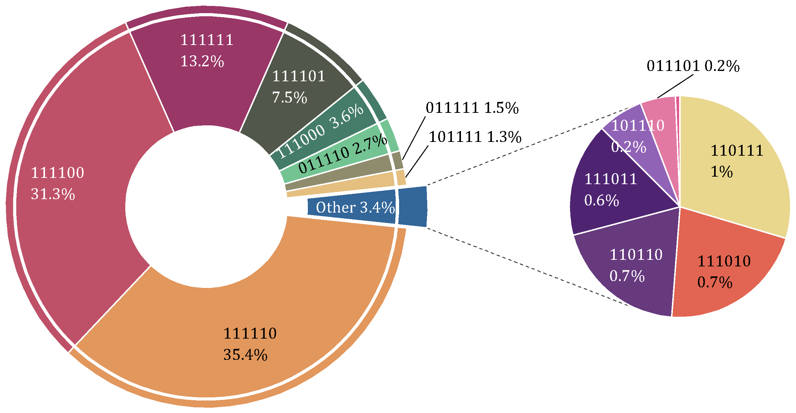
| Combination mode of coal mills | - | 3–6 |
| Variable Description | Symbol | Operation Range |
|---|---|---|
| Main steam flow (t/h) | MSFlow | [1091.99, 1991.28] |
| Ambient temperature (°C) | AT | [−4.38, 38.09] |
| Lower heating value of coal (KJ/kg) | Qnet,ar | [19,699, 24,758] |
| Coal mill combination | - | 111,110 |
| Condition Variables | Parameter Description | Cluster Result | ||||
|---|---|---|---|---|---|---|
| Main steam flow | [KMSFlow] | 17 | ||||
| Cluster center | 1259.81 | 1319.76 | 1373.22 | 1959.59 | ||
| Cluster interval | [1203.8, 1289.7] | [1289.82, 1346.49] | [1346.5, 1387.08] | [1906.13, 1991.28] | ||
| Number of samples | 2831 | 5241 | 8714 | 1090 | ||
| Ambient temperature | [KAT] | 10 | ||||
| Cluster center | 0.04 | 3.63 | 6.83 | 32.59 | ||
| Cluster interval | [−4.38, 1.83] | [1.84, 5.23] | [5.24, 8.87] | [30.75, 38.09] | ||
| Number of samples | 11,767 | 16,391 | 18,277 | 8786 | ||
| Low calorific value | [KQnet,ar] | 5 | ||||
| Cluster center | 19,989 | 20,805 | 22,330 | 23,243 | 24,273 | |
| Cluster interval | [19,699, 20,375] | [20,452, 21,557] | [21,600, 22,758] | [22,795, 23,736] | [23,763, 24,758] | |
| Number of samples | 7652 | 22,262 | 34,785 | 46,612 | 31,308 | |
| Order | 1 | 2 | 3 | 4 | 5 | 6 | 7 | 8 | 9 | 10 | 11 | 12 | 13 | 14 | 15 | 16 | 17 | 18 |
| Entry | ||||||||||||||||||
| Removal | ||||||||||||||||||
| Order | 19 | 20 | 21 | 22 | 23 | 24 | 25 | 26 | 27 | 28 | 29 | 30 | 31 | 32 | 33 | 34 | 35 | 36 |
| Entry | ||||||||||||||||||
| Removal |
| Operating Status | Operation Time | MSFlow (t/h) | Samples (min) |
|---|---|---|---|
| Exit | 1 December 2022 10:00–2 December 2022 10:00 | [1350, 1950] | 1440 |
| Input | 2 December 2022 15:00–3 December 2022 15:00 | [1300, 1750] | 1440 |
| Operating Status | Proximate Analysis (wt%, as Received) | LHVC (KJ/kg) | UBC in Fly Ash (%) | |||
|---|---|---|---|---|---|---|
| Moisture | Volatile Matter | Fixed Carbon | Ash | |||
| Exit | 7.23 | 9.86 | 56.91 | 26.00 | 23,066 | 11.63 |
| Input | 6.35 | 9.27 | 59.73 | 24.65 | 23,888 | 9.61 |
Disclaimer/Publisher’s Note: The statements, opinions and data contained in all publications are solely those of the individual author(s) and contributor(s) and not of MDPI and/or the editor(s). MDPI and/or the editor(s) disclaim responsibility for any injury to people or property resulting from any ideas, methods, instructions or products referred to in the content. |
© 2023 by the authors. Licensee MDPI, Basel, Switzerland. This article is an open access article distributed under the terms and conditions of the Creative Commons Attribution (CC BY) license (https://creativecommons.org/licenses/by/4.0/).
Share and Cite
Wang, Z.; Yao, G.; Xue, W.; Cao, S.; Xu, S.; Peng, X. A Data-Driven Approach for the Ultra-Supercritical Boiler Combustion Optimization Considering Ambient Temperature Variation: A Case Study in China. Processes 2023, 11, 2889. https://doi.org/10.3390/pr11102889
Wang Z, Yao G, Xue W, Cao S, Xu S, Peng X. A Data-Driven Approach for the Ultra-Supercritical Boiler Combustion Optimization Considering Ambient Temperature Variation: A Case Study in China. Processes. 2023; 11(10):2889. https://doi.org/10.3390/pr11102889
Chicago/Turabian StyleWang, Zhi, Guojia Yao, Wenyuan Xue, Shengxian Cao, Shiming Xu, and Xianyong Peng. 2023. "A Data-Driven Approach for the Ultra-Supercritical Boiler Combustion Optimization Considering Ambient Temperature Variation: A Case Study in China" Processes 11, no. 10: 2889. https://doi.org/10.3390/pr11102889