Article

Study on Transient Flow and Dynamic Characteristics of Dual Disc Check Valve Mounted in Pipeline System during Opening and Closing

Key Laboratory of Hydraulic Machinery Transient, MOE, Wuhan University, Wuhan 430072, China
*
Authors to whom correspondence should be addressed.
Processes 2022, 10(9), 1892; https://doi.org/10.3390/pr10091892
Submission received: 3 August 2022 / Revised: 7 September 2022 / Accepted: 12 September 2022 / Published: 18 September 2022
(This article belongs to the Section Chemical Processes and Systems)

Abstract

:
Check valves are used extensively in industrial piping systems. Based on dynamic mesh technology, this study uses the RNG k-ε turbulence model to numerically calculate the dual disc check valve’s three-dimensional transient flow. The dynamic characteristics of the check valve in the pipeline system are also experimentally studied. To this end, the two discs are opened synchronously during the valve-opening process, including four stages: opening discs at a constant angular velocity, opening slowing down discs, slowly returning discs to the balance point, and discs maintaining oscillation. However, the movements of the two discs are asynchronous in the valve-closing process. As the downstream pressure increases, the valve disc begins to close, and the flow gradually stops; reverse flow takes shape, and the reverse flow stops until the discs are fully closed, and slamming of the check valve occurs. The non-dimensional dynamic characteristic curve of this type of dual disc check valve has a slope of about 1.624, which mirrors the response of the check valve closing to the occurrence of the water hammer in the system. Knowing the dynamic behavior can be convenient in designing and selecting a check valve and regulating piping system working conditions.

1. Introduction

In modern industrial production, fluid-related industries such as petrochemicals, water conservancy, shipbuilding, and electric power are inseparable from complex piping systems. The safe and stable operation of piping systems has always aroused general interest. As an indispensable component of the piping system, the check valve can prevent backflow and play a vital role in water hammer protection in the piping system. However, the check valve increases the hydraulic loss of the piping system (resistance characteristics), and instantaneous reverse flow occurs during the closing process of the check valve, which may cause the valve to slam (dynamic characteristics) [1,2].
Scholars have conducted research on check valves. In 1980, G. A. Provoost conducted experimental research on two types of check valves (ball valves and swing valves) and pointed out that considering the dynamic characteristics of check valves, the fluid velocity gradient with time is crucial [3]. In 1989, A. R. D. Thorley proposed a dimensionless dynamic characteristic curve of a check valve based on a theoretical derivation method. He believed that the acceptable maximum reverse flow velocity through the check valve could be regarded as a controlling parameter in the valve calculation program.
In addition, the average deceleration of the fluid provides an indispensable foundation for selecting the most suitable check valve [4]. In 1996, K. K. Botros et al. studied the influence of the dynamic characteristic curve of the check valve on the circulation system of a centrifugal compressor. They deemed that the maximum slope of the curve determines the maximum tolerance the compressor/circulation system allows for reverse flow through the check valve [5]. In 1999, Patrick J. Purcell investigated the “slamming” problem of the check valve in the chief pump-pressurization system with an air tank through experiments and numerical methods. He proposed that throttling the outflow from the air container can minimize valve slamming during the negative water hammer phase of the transient cycle system. However, excessive throttling of the outflux may cause cavitation in the main piping [6]. Guohua. Li and Jim C. P. Liou determined the influence of hydraulic torque on the swing check valve disc on the valve–fluid dynamic interaction. They believed that the hydraulic torque involved the torque induced by the flow around the stationary disk and the torque generated by the rotation of the disk [7]. Based on the RNG k-ε turbulence model, Stefano Sibilla and Mario Gallati research the pressure drops and flow rate coefficient of the valve during the steady-state flow of the nozzle check valve at different positions and the unsteady flow in the valve plug transient opening. The researchers indicated that the flow separation occurred downstream of the valve plug and lasted after the valve was opened, which caused the valve to increase the additional pressure drop in the first half of the stroke, which deviated from the quasi-steady-state characteristic curve of the valve [8].
K. K. Botros studied the effects of various spring characteristics and stiffness of the nozzle check valve on the flow characteristics of the compressor station. The researcher advanced that the valve disk will not be at the fully open position when the spring force is higher than the maximum hydrodynamic force at the minimum flow rate. At this moment, the disk may flutter, and the internal components of the valve cyclically impact each other at high speed. That could lead to the check valve self destructing. He also proposed selecting the spring force and stiffness according to the relationship between the flow characteristics of the valve fully opened and the compressor performance curve [9].
Zhida Yang et al. performed CFD transient calculations on the closing process of the reverse check valve in the experimental loop of the nuclear power plant under the reverse flow pressure difference. These researchers brought to light that the reverse check valve can effectively suppress the water hammer phenomenon during the switching transition of the parallel double pumps [10]. Zhounian Lai et al. numerically simulated the transient opening of the dual disc check valve. They hold that the discs will not move until the inlet velocity increases to a fixed value. The discs open with the flow velocity enhancing, and the pressure drop begins to rise. When the valve flap reaches the maximum opening, the pressure drop rockets, and the flow rate continues to boost [11].
Nam-Seok Kim and Yong-Hoon Jeong used four different dynamic grid techniques to calculate the dynamic characteristics of the swing check valve during the closing period. The results show that the velocity distribution at the outlet of each method is similar before the valve is almost closed. When the valve has fully closed, the prediction of the inflow fluid velocity is different [12]. Zhounian Lai et al. carried out a three-dimensional transient state numerical simulation of a dual disc check valve and employed overlapping meshes to ensure the disc’s complete closing and pressure fluctuations were accurately captured. They explained the influence of the system outlet pressure, initial flow rate, and upstream pump closing speed on the pressure fluctuation caused by the closing of the check valve [13].
The current study mainly focuses on the numerical calculation of the internal flow characteristics of the check valves and their influence on the dynamic system. However, there are few studies on the valve plate–fluid interaction during the opening and closing process of the check valves and the dynamic characteristics of the check valves during the transition process of the pipeline system. For the dual disc check valve, this study adopts dynamic mesh technology to research the valve disc–fluid interaction caused by the opening and closing of the check valve in detail; moreover, it discusses the dynamic characteristic of the check valve during the transition process of the piping system by an available test bench built. The paper reveals the development of the flow field during the opening and closing of the double-disc check valve, as well as the pressure change characteristics of the piping system upstream and downstream of the valve. The research will provide some recommendations for engineers in the design and selection of check valves, water hammer protection, and working condition adjustment of the pipeline system.

2. Numerical Calculation Method

2.1. Scheme Design

This study has six opening schemes and four closing schemes of the dual disc check valve. Table 1 shows the valve opening flow rate under each opening scheme. Table 2 shows the upstream and downstream pressure of the valve (opening the check valve, when the fluid maintains a stable flow, in the direction of flow, the front of the check valve is upstream, and the back is downstream). The upstream pressure is a constant value, but the downstream pressure changes with the flow time.

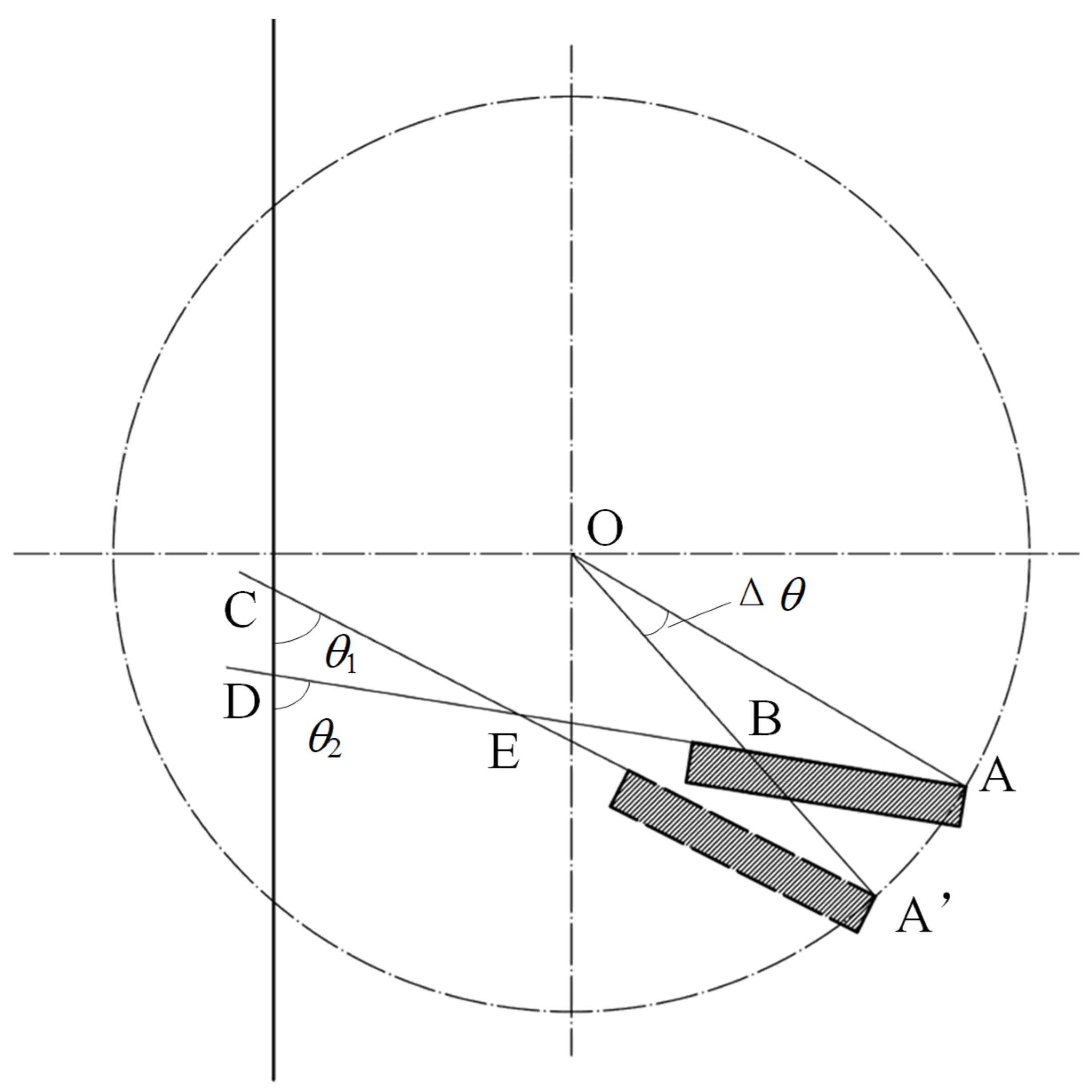
2.2. Geometric Model of Dual Disc Check Valve

The two discs of the dual disc check valve are fixed by a valve stem and springs and can rotate around the stem. When installing the valve, ensure that the axis of rotation is consistent with the direction of gravity. When the upstream fluid (the positive direction of the y-axis in Figure 1 points upstream) washes out the front of the valve plate, the check valve opens, as shown in Figure 1b. When the upstream piping system fails, the downstream fluid will backflow, and the check valve will be closed (Figure 1a).
When the valve plate is in the fully closed position, the artificial gap between the valve seat and the valve plate appends to ensure the continuity of the calculating flow domain. The volume meshes at this gap become a porous medium, which can almost prevent fluid flow [11,12].
Figure 2 shows the schematic diagram of the valve disc movement. Because the motion of the valve disc approximates a rigid body rotation, the disc is almost deformation-free, ∠OAD = ∠OA’C.
In addition, to facilitate the test measurement, the valve disc opening angle is defined as θ, θ = θ2θ1 = ∠CED = ∠AEA’, ∠ABO = ∠A’BE.
In the triangle △OAB, ∠AEA’ = 180° − ∠OA’C−∠A’BE. In the triangle △OAB, ∠AOA’ = 180° − ∠OAD−∠ABO.
Therefore, ∠AEA’ = ∠AOA’; that is, θ = Δθ (angular displacement of valve disc).
When the initial opening degree is 0, the instantaneous opening angle of the valve disc is equal to the instantaneous angular displacement of the valve disc movement.

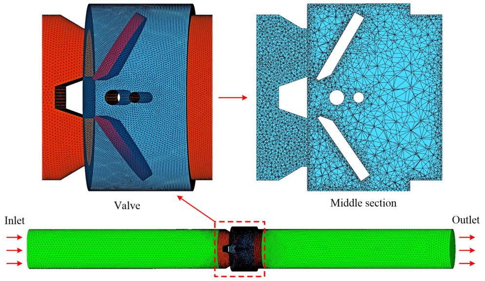
2.3. Whole Fluid Domain Meshing

Using 3D modeling software pro/E constructs the whole flow passage of the dual disc check valve. Numerical calculations were performed using ANSYS/Fluent software. To ensure the availability of the numerical model, the upstream and downstream sections of the valve, respectively, extend five times the nominal diameter of the valve. As shown in Figure 3, adopting unstructured tetrahedral cells meshes the whole flow passage. The meshes of the fluid domains of the great curvature transition flow passage and the near-wall carry out refined processing. This numerical simulation uses a dynamic mesh technique, where the valve disc is in rapid motion, causing constant changes in the fluid domain. Unstructured meshes allow better mesh reconstruction and better adaptation to the fluid domains. In addition, it becomes easier to refine the local meshes. As shown in Figure 4, the mesh cells of different sizes carried out mesh independence checks, considering the calculation accuracy and efficiency of the computer, and the initial total number of cells was determined to be about five million. The dynamic mesh whose generation method adopts elastic smoothing and local reconstruction has a minimum cell size of 0.5 mm and a maximum distortion rate of 0.75.

2.4. Governing Equation

The flow control equation of this dual disc check valve adopts a continuous equation and Reynolds time average N-S (Navier–Stokes) equation. The flow channel of the valve has a complex structure causing many vortex flows, so the RNG k-ε turbulence model is adopted [8,10,11,12,13]. The valve disc motion equation employs Newton’s second law. The fluid domains swept by the discs use a dynamic mesh equation.
  • Continuous equation
ρ t + ( ρ u i ) x i = 0
where ρ is the fluid density, u is the fluid velocity. The subscript “i” represents the component of the tensor in the coordinate system.
  • Reynolds time average N-S equation [14]
( ρ u i ) t + ( ρ u i u j ) x j = p x i + x j [ μ ( u i x j + u j x i 2 3 δ ij u l x l ) ] + x j ( ρ u i u j ¯ )
where p is the fluid pressure, μ is the dynamic viscosity coefficient of the fluid, and δij is the Kronecker number. The subscripts “i, j, l” represent the components of the tensor in the coordinate system.
ρ u i u j ¯ = μ t ( u i x j + u j x i ) 2 3 ( ρ k + μ t u k x k ) δ ij
where μt is the turbulent eddy viscosity coefficient, k is the turbulent kinetic energy.
  • RNG k-ε turbulence model [15]
( ρ k ) t + ( ρ k u i ) x i = x j ( α k μ eff k x j ) + G k + G b ρ ε Y M + S k
( ρ ε ) t + ( ρ ε u i ) x i = x j ( α ε μ eff ε x j ) + C 1 ε ε k ( G k + C 3 ε G b ) C 2 ε ρ ε 2 k + S ε
where ε is turbulence dissipation rate; αk = αε = 1.39, μeff = μ + μt, μ t = ρ C μ k 2 ε .
Gb is the production term of turbulent kinetic energy caused by buoyancy; YM is compressible turbulent pulsation expansion term; Gk is stress source term caused by velocity gradient; Sk and Sε are user-defined source terms;
C 1 ε = C 1 ε η 1 η / η 0 1 + β η 3 , η = 2 E ij E ij k ε , E ij = 1 2 ( u i x j + u j x i )
C = 1.42, C = 1.68, C = 0.09, β = 0.012, η0 = 4.377
  • Dynamic mesh equation
Concerning dynamic meshes, the integral form of the conservation equation for a general scalar ϕ, on an arbitrary control volume V, whose boundary is moving can be written as:
d d t V ρ ϕ d V + V ρ ϕ ( u u g ) d A = V Γ ϕ d A + V S ϕ d V
where ∂V is used to represent the boundary of the control volume; u is the flow velocity vector; u g is the mesh velocity of the moving mesh; Γ is the diffusion coefficient; Sϕ is the source term of ϕ.
  • Newton’s second law
I d 2 θ d t 2 = T P + T V ± T N T f
where θ is the opening angle of the discs; I is the moment of inertia of the discs; TP is the moment of the hydrostatic pressure; TV is the moment of the fluid impact force; TN is the spring torque. The torque is “−“ when opening the valve and “+” when closing the valve; Tf is the friction torque between the discs and the stem, and it is relatively small compared to other torques and can be ignored.
T P = Δ p A R
where ∆p is the static pressure difference between the two sides of the discs; A is the area of one side of the disc, and R is the distance from the center of mass of the disc to the axis of rotation.
T V = ρ q u R cos θ
where q is the flow rate; u is the flow velocity of the fluid.
T N = T p r e l o a d + T θ
where Tpreload is the spring pre-tightening torque; T is the spring stiffness.

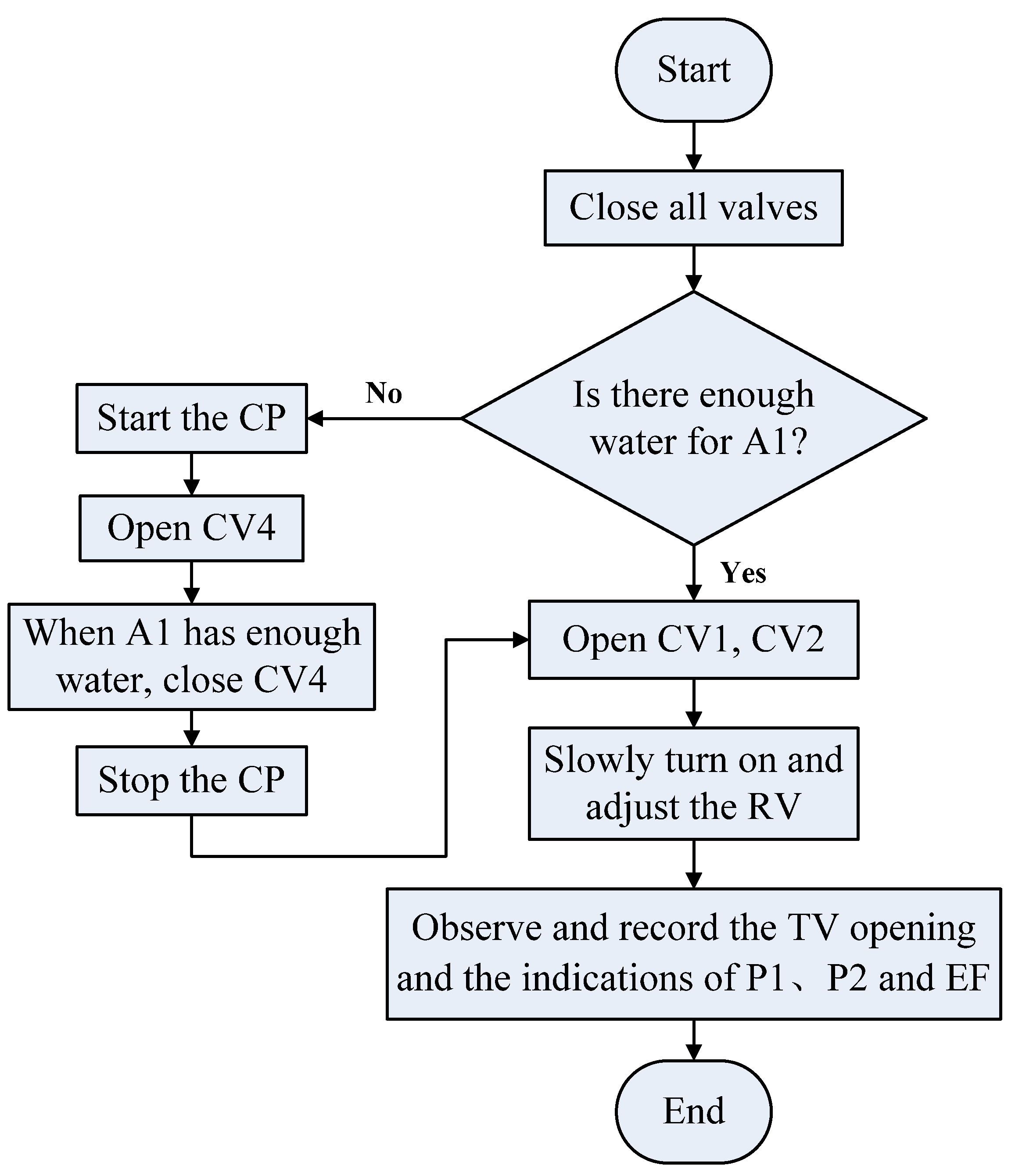
2.5. Boundary Conditions and Solving Methods

  • Boundary condition of the opening valve
The inlet boundary condition adopts the mass-flow inlet (see Formula (11)), the value is flowrate in Table 1, and the outlet boundary condition employs outflow.
ρ v n = m A in
where m is total mass flow; Ain is inlet cross-sectional area; vn is normal velocity.
  • Boundary condition of closing valve
The inlet boundary condition adopts the pressure inlet (see Formula (12)), and the value is the upstream pressure in Table 2. The outlet boundary condition employs the pressure outlet, and the value is the downstream pressure in Table 2. The pressure change with the flow time is realized through a user-defined function.
p in = p S + 0.5 ρ v i n
where pin is inlet total pressure; pS is static pressure; vin is inlet velocity.
  • Wall condition
The wall condition adopts the no-slip and the standard wall function [16].
  • Solution methods
The coupling of pressure and velocity is solved using the SIMPLE algorithm, the time step of the transient calculation is 10−4 s, and each time step is iteratively calculated twenty times. Figure 5 shows the change curves of the residual with the number of iterations. As can be seen, the residuals of fluid velocity are all less than 10−3, meeting the accuracy of engineering calculation.

3. Experimental Apparatus and Procedures

3.1. Experimental Apparatus

As shown in Figure 6, the main components of the testing system of the dual disc check valve include a high water pool A1 (20 m from the tested valve), low water pool A2, centrifugal pump CP (rated head: 50 m, rated flow: 200 m3/h), pressure sensor P1/P2 (range: −0.1–1.5 MPa, accuracy: 0.25%, the measured pressure points are set at a position of 5 times the diameter of the pipe (200 mm) from the tested valve), electromagnetic flowmeter EF (specification: DN200, range: 0–300 m3/h, accuracy: 0.21%), data acquisition system (sampling frequency: 6400 Hz), regulating valve RV, control valve CV, tested dual disc check valve TV. Figure 7 shows the built experimental setup.

3.2. Experimental Procedures

  • Resistance characteristics experiment
It is necessary to measure the flow rate, maximum opening, and pressure drop when the check valve opens and draw other relationship curves with the flow rate. Figure 8 is a test flowchart of the dual disc check valve in the opening process.
  • Dynamic behavior test
The water hammer has been generated since the valve is closed, but when the valve is fully closed, the reverse flow stops, and the amplitude of the water hammer reaches the maximum. The water hammer pressurization satisfies the Joukousky equation [2,17,18]:
Δ H = a Δ v g
Δ P = ρ g Δ H = ρ a Δ v
Δ v = 0 v R
According to Formulas (13)–(15):
v R = Δ P / ρ a
where ΔP is the pressure difference between the initial pressure and the peak water hammer pressure; Δv is the change of fluid velocity; ρ is the fluid density; a is the water hammer wave speed, when the ratio of pipe diameter (200 mm) to pipe wall thickness (2 mm) is 100, taken as 1000 m/s in the steel pipe [19]. vR is the maximum reversal flow velocity.
The fluid deceleration of piping system dv/dt:
d v / d t = | 0 v 0 / t 0 | = v 0 / t 0 = 4 Q 0 / π t 0 d 2
where v0 is the flow velocity of steady flow in the initial state; Q0 is the flow rate of steady flow in the initial state; t0 is the time for the fluid velocity to decrease from v0 to 0; d is the diameter of the downstream pipeline.
It is almost impossible to accurately measure the maximum reversal flow velocity using an electromagnetic flowmeter [20]. This study indirectly measures vR by Formula (16) to measure ΔP. The measured Q0 and t calculate dv/dt by Formula (17). The (dv/dt-vR) curve drawn is the dynamic characteristic of the check valve. Figure 9 is a test flowchart of the dynamic behavior of the valve-closing process.

4. Results and Discussion

4.1. The Opening Process of the Check Valve

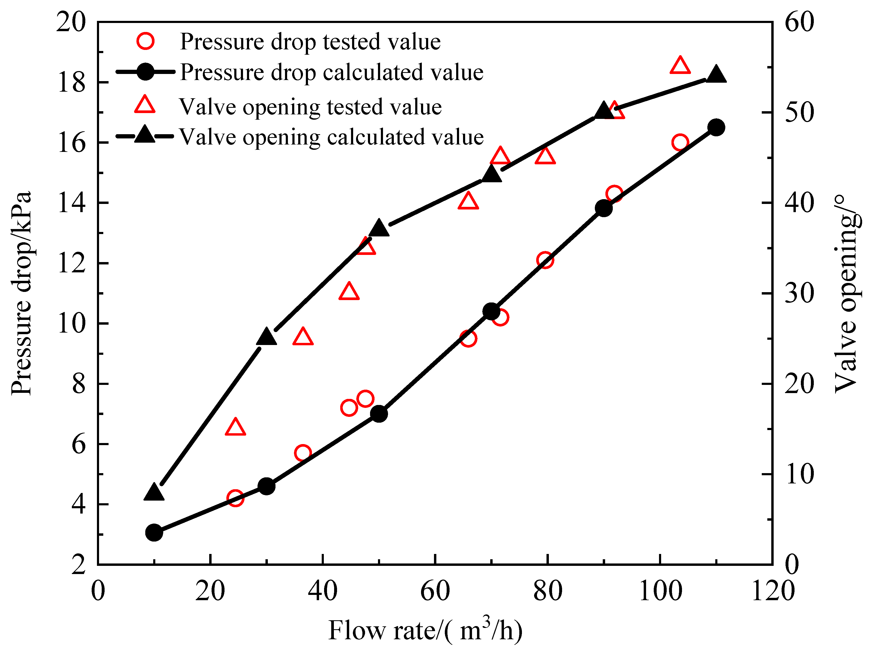
4.1.1. Resistance Characteristics

When the fluid in the upstream pipeline flows through the check valve and acts on the valve discs, the valve discs are opened against the restraining force of the spring, resulting in the hydraulic loss (resistance characteristics). Figure 10 shows the relationship between pressure difference and opening with the flow rate when the dual disc check valve opens. As can be seen, when the flow rate is higher than 50 m3/h, the numerical calculation results are very consistent with the test results. However, when the flow rate is less than 50 m3/h, the calculated value of valve opening is slightly larger than the test value, and the maximum error is less than 2°. That is because the numerical calculation ignores the mechanical friction between the valve discs and the stem, or the systematic test error is relatively large when the valve opening is small under a small flow. In general, compared with the tested value, this calculation result is reliable and meets the engineering calculation requirements. It was demonstrated that the established numerical model is quite reliable in calculating the study.
As shown in Figure 10, the pressure drop increases significantly as the flow rate grows. That is because when the flow rate increases, the average flow velocity escalates; namely, the kinetic energy loss grows when the fluid passes through the valve, which causes the pressure drop between the two sides of the valve to enhance. However, as the flow rate increases, the valve opening angle rises remarkably to 35°, then the flow rate continues to increase, and the valve opening angle improves slowly. The following reasons can explain this situation. According to Formulas (9) and (10), the impact torque of the fluid acting on the valve discs under a few flow rates is small and needs to overcome the spring preload torque to open the valve discs. When the valve opening is small, it has less negative feedback on the impact torque of the fluid and spring torque. As the flow rate increases, the impact torque of the fluid grows significantly, and the valve disc opening enhances remarkably. However, when the flow rate increases to 50 m3/h, the valve disc opening is 35°. At this time, the valve opening has a vigorous negative feedback on the impact torque of the fluid and spring torque. So the flow rate continues to increase, the impact torque of the fluid improves scarcely, but the spring torque significantly increases, and the valve disc opening grows barely.

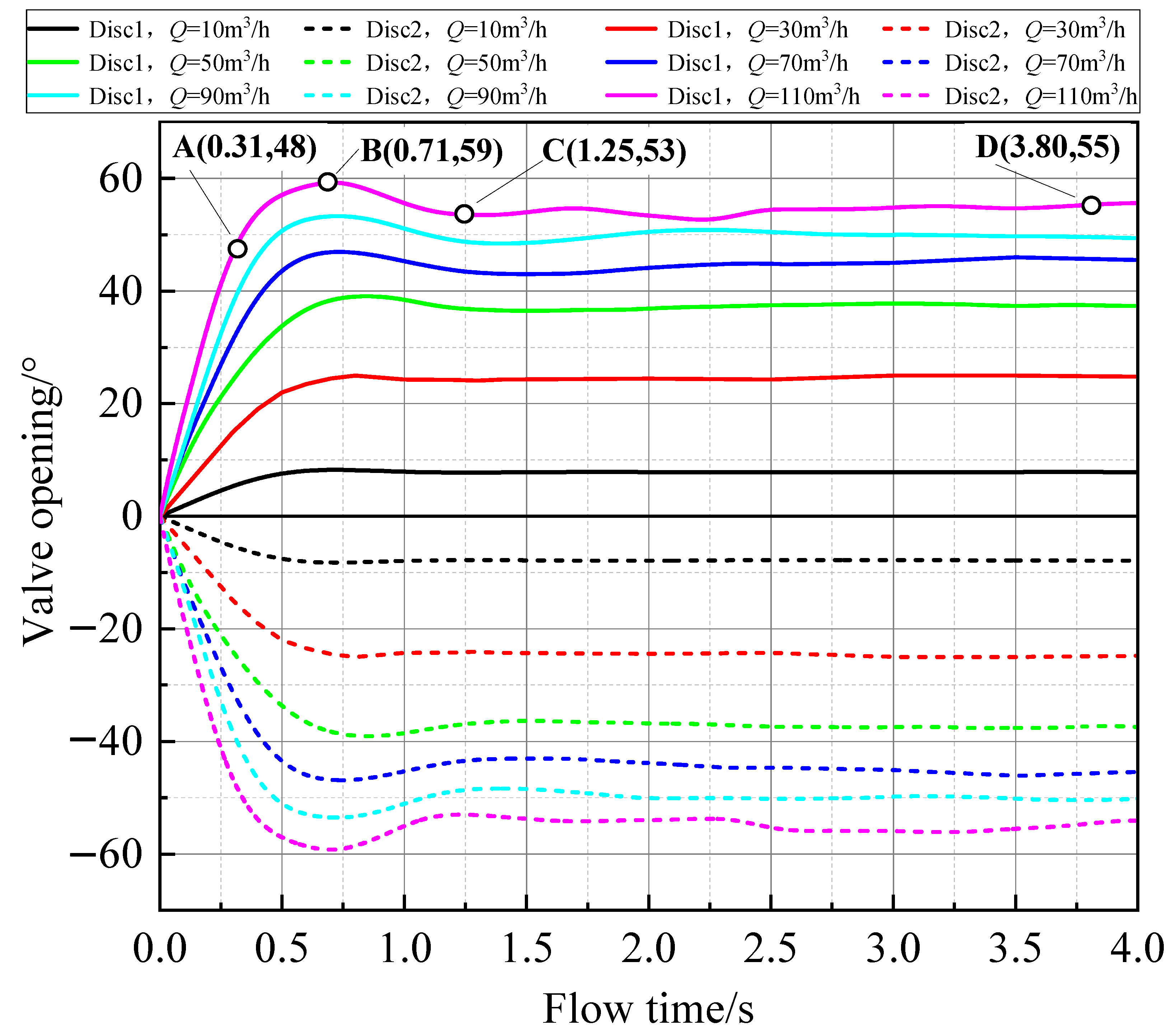
4.1.2. Transient Characteristics

Figure 11 shows the transient curve of the opening angle change of the dual disc check valve during the opening process under different flow rates. As can be seen, the two discs are opened synchronously during the valve opening process, except that the direction of rotation is opposite. The change of the valve disc opening with flow time has four stages.
0A stage (opening the discs at a constant angular velocity): The valve opening increases linearly with time, and the slope of the curve remains the same, proving the disc’s angular velocity remains the same.
AB stage (opening the discs at a slower angular velocity): The slope of the curve decreases continuously, which shows that the valve discs slowly open with time. The discs reach the maximum opening under this flow at point B.
BC stage (the discs slowly return to the balance point): The valve disc slowly returns from point B (the maximum opening) to the balance point (point C).
CD stage (the discs maintaining oscillation): The valve disc keeps slightly oscillating near the balance point over time.
The following reasons can explain this phenomenon. When a constant flow rate of upstream fluid flows to the front of the valve discs, the impact torque and static pressure torque on the valve disc front is higher than the spring torque of the valve disc back, and the valve discs tend to open. When the valve discs initially open, the static pressure moments in their front and back have the same magnitude and opposite directions. The static pressure moment does not work on the valve discs, and the impact and spring torque are not much different, so discs open at a constant angular velocity. As the opening increases, the impact torque decreases, and the spring torque increases (as shown in Formulas (9) and (10)). Due to the inertia of the valve discs, the valve discs decelerate to open. When the angular velocity of the valve discs decrease to 0, the opening degree reaches the maximum value. At this moment, the spring and impact torque is unbalanced (the two trade off each other), and the valve discs return to a closed state at a variable angular velocity. When each reaches equilibrium, the valve discs reach the equilibrium point.
Figure 12 is the instantaneous flow field diagram of the valve opening, Scheme 6. As can be seen, the downstream flow is relatively smooth during the valve disc opening at a constant angular velocity. After that, when the fluid flows around the valve disc, a vortex street is formed behind the valve discs, the flow field is relatively turbulent; it can be clearly seen that the vortex generated after the valve disc eventually returns to the vicinity of the valve disc. The process of vortex moving forms pressure pulsation in the flow field, which causes the valve disc’s torque to be unbalanced, and the valve disc oscillates near the equilibrium point.
As shown in Figure 11, when the flow rate is different, each stage of the valve opening process is different. In the 0A stage, with the flow rate increase, the valve disc’s opening angular velocity increases, and the valve is opened more quickly. In the AB stage, with the growth of flow rate, the valve opening increases, and the curve’s curvature enlarges (the angular acceleration enhances). In the BC stage, with the growth of flow rate, the return of opening increases. In the CD stage, with the rise in flow rate, the oscillation amplitude of the opening increases.
That is because the flow rate increases, the impact torque of the fluid grows, the angular velocity of the valve plate opening is reduced, the moment of inertia generated by the movement of the discs strengthens, and the opening change increases during the disc decelerating opening and variable speed return closing. Moreover, as the flow rate increases, the pressure pulsation caused by the vortex shedding intensifies, and the valve disc oscillation amplifies.

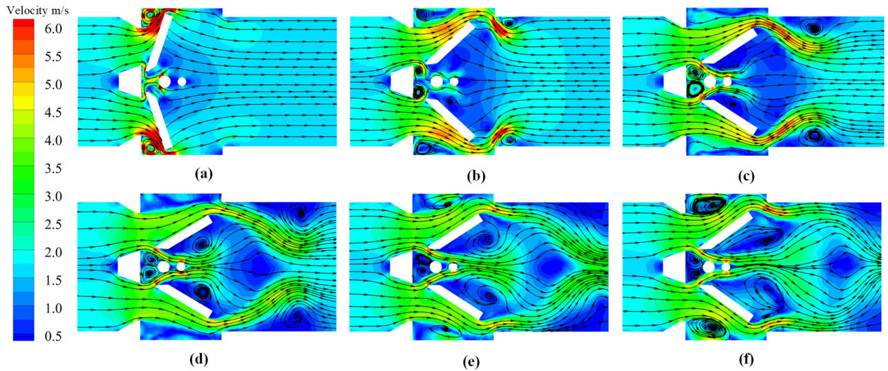
4.2. The Closing Process of the Check Valve

When the check valve is fully open, the fluid in the pipeline flows steadily, and the upstream pressure is higher than the downstream pressure. When an accident occurs in the upstream pipe and equipment, the upstream pressure decreases and is lower than the downstream pressure, which leads to fluid backflow, and the check valve will be closed. In this study, to explore the closing law of the dual disc check valve, gradually increasing the downstream pressure makes it higher than the upstream pressure, which results in closure of the valve.

Transient Characteristics

Figure 13 shows the opening change with the flow time during the closing process of the check valve. As can be seen, the two discs are asynchronously closed with the passing of the flow time. The other disc begins to close before one of the discs is closed for a short period, but their required close time is almost the same. During the valve-closing process, the slope of the curve gradually increases (the angular velocity of the discs continues to enhance), and the two discs accelerate to close until they are fully closed.
That is because when the downstream pressure gradually increases, the flow is blocked, forming a complex vortex and reverse flow, resulting in asymmetric flow distribution downstream. The hydrodynamics acting on the back of the two discs changes non-uniformly but is almost equivalent, so the discs are asynchronously closed, and their closing times are nearly the same. As the downstream pressure gradually increases, the torques acted on the discs become higher, and the discs continue to accelerate to close.
Comparing the four valve-closing schemes, the trends of opening with time are nearly identical. However, the closing time of the disc becomes shorter when the downstream pressure increases faster. That is because the downstream pressure improves rapidly, the hydraulic torque on the back of the discs increases quickly, and the disc closing angular velocity becomes faster.
Figure 14 shows the transient change of the flow field in the valve-closing Scheme 1. As can be seen, the fluid flows steadily from upstream to downstream in the valve fully opened. There are core flow areas near the pipe wall of the valve discs’ sides and symmetrical vortex flows near the center of the pipe downstream (see Figure 14a). With the increase of the downstream pressure, the vortex area extends, the flow velocity reduces significantly, and the flow is almost stagnant (see the red mark in Figure 14b). As the downstream pressure continues to increase, disc 2 begins to close, and the downstream fluid accelerates backflow (see the red mark in Figure 14c). The core flow area appears at the center of the pipe, and the asymmetrical distributing vortex areas approach the pipe wall (see Figure 14c). As the downstream fluid continues to backflow rapidly, two discs move to different positions, but the disc 1 is greater than the disc 2 opening, the core flow area extends, and the vortex areas continue to decrease (see Figure 14d,e). The flow is almost stagnant when the discs are fully closed (see Figure 14f).
There are some reasons for this characteristic. When the valve fully opens, the flow passage is symmetrical. The upstream high-pressure fluid flows around the discs and forms the symmetrically distributed vortexes behind the discs, forcing the core flow area to move near the pipe wall. However, when the continuously increasing downstream pressure is higher than the upstream pressure, due to the reverse pressure gradient, flow separation occurs, resulting in asymmetrically distributed vortexes expanding. The vortex areas push out the mainstream, increasing hydraulic loss and decreasing flow velocity. When the downstream pressure increases continuously, reverse flow occurs as the two discs asynchronously accelerate to close. The downstream high-pressure fluid destroys the vortexes behind the discs and squeezes them near the pipe wall. The center of the pipe becomes the core area of flow, and the flow becomes smoother and more orderly.

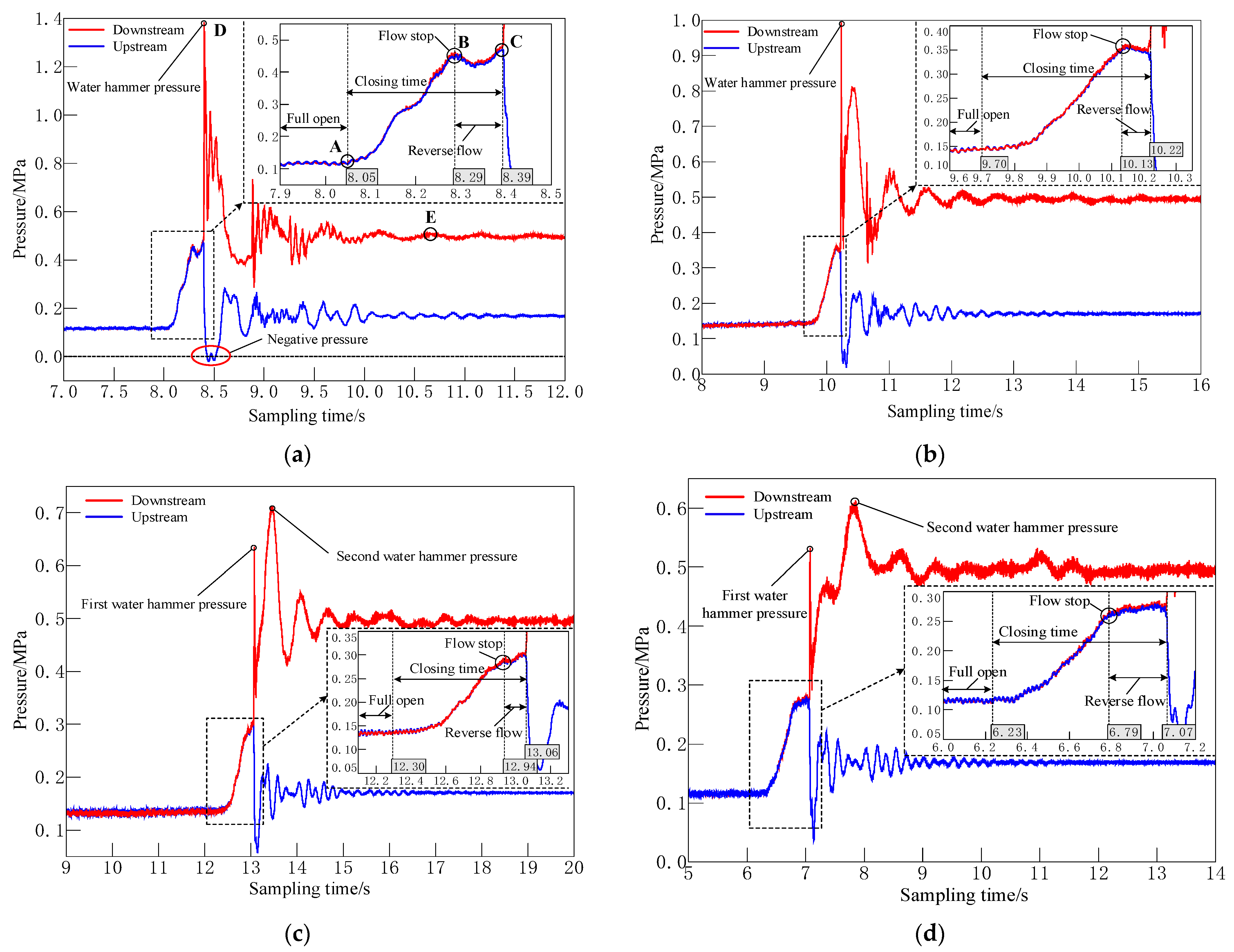
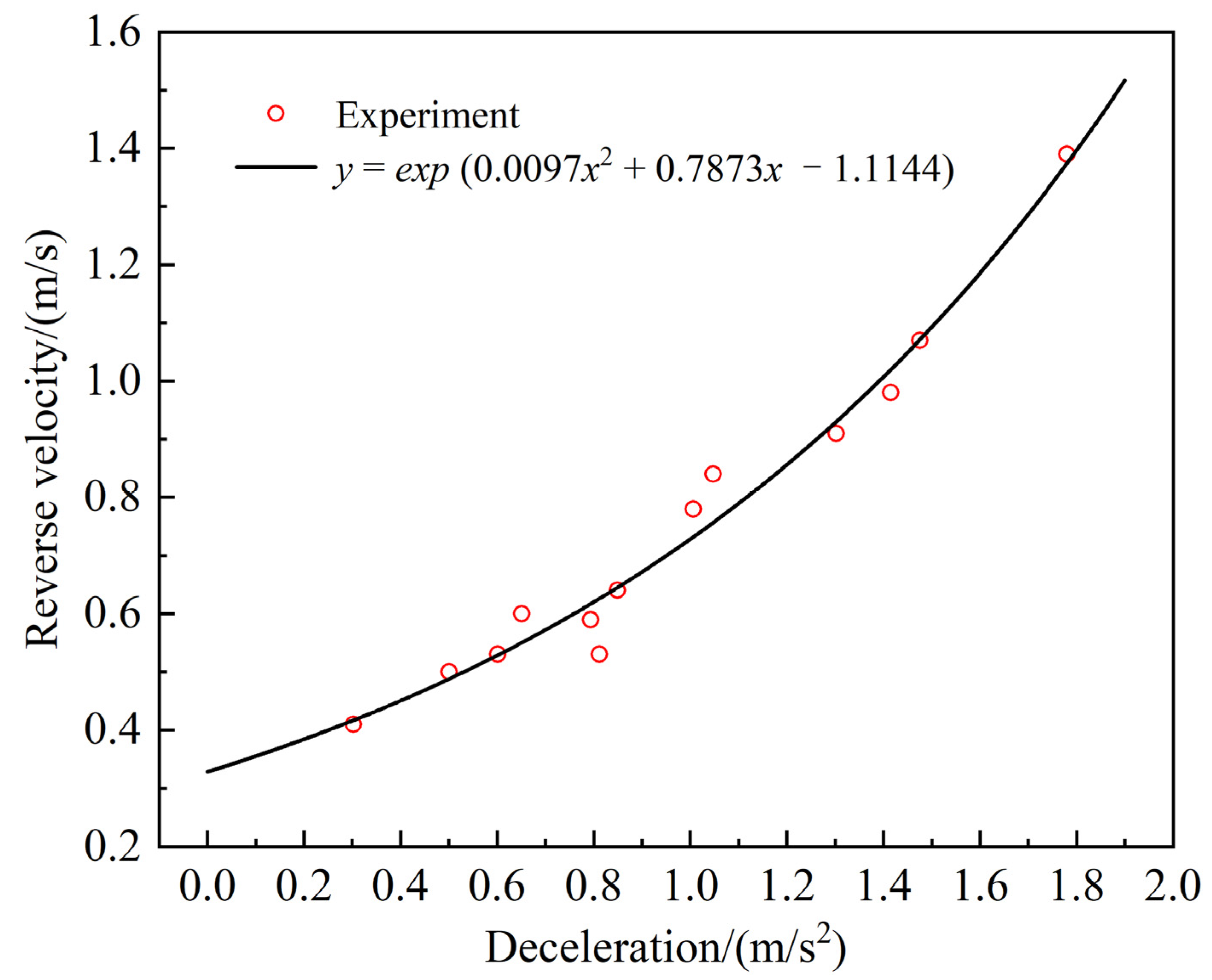
4.3. The Test of Dynamic Characteristics of Check Valve

Figure 15 shows the transient pressure-tested curves at different valve-closing times. As can be seen, when the valve is in the fully open position, the pressure upstream and downstream is almost equal and remains constant. As shown in Figure 15a, the downstream pressure begins increasing at point A and transmits to the upstream through the check valve. In the AB stage, the upstream and downstream pressures increase simultaneously, and the fluid decelerates with the check valve closing gradually. At point B, the upstream and downstream pressures no longer increase, and the flow stops. In the BC stage, the upstream and downstream pressures fluctuate slightly or remain constant with the check valve’s closing, and a reversal flow occurs whose velocity continues to increase. At point C, the flow stops instantaneously with the check valve slamming, the upstream pressure reduces drastically, and gradually returns to the pressure value of the high water tank. However, the downstream pressure increases sharply with the water hammer beginning to occur at point C, reaches the pressure peak of the water hammer at point D, then gradually subsides and stabilizes at point E [21,22].
By comparing the transient pressure curves in different closing times, as can be seen, the shorter the closing time, the greater the peak pressure of the water hammer. As shown in Figure 15a, when closing time becomes short, a direct water hammer occurs downstream, and the pressure peak of the water hammer is far higher. The upstream water column separates and forms air pockets after the valve is closed, which leads to instantaneous negative pressure and cavitation [23]. As shown in Figure 15c,d, the closing time is far longer, and the secondary water hammer superimposes the reflected wave of the primary water hammer, resulting in the indirect water hammer downstream, which causes the peak of the secondary water hammer to be higher than the primary.
Figure 16 is the dynamic characteristic curve of the dual disc check valve. As can be seen, the maximum reverse flow velocity of the check valve increases as the fluid deceleration of the pipeline system increases, and the changing trend fits well with the exponential functions y = exp (0.0097x2 + 0.7873x − 1.1144). When the deceleration of the pipeline system is a definite value, the smaller the maximum reverse flow velocity, the lower the water hammer pressure peak causing the check valve to close, and the better the water hammer protection performance of the check valve. Figure 16 reflects that this check valve has better water hammer-protection performance when deceleration is lower.
It is necessary to analyze the dimensionless variables to study the dynamic characteristics of dual disc check valves with similar structures. Using the ratio of vR and v0 obtains the dimensionless maximum reverse flow velocity v * (see Formula (18)). In the same way, using the rate of dv/dt and v02/d achieves the dimensionless fluid deceleration A * (see Formula (19)). Finally, the A *-v * curve is the dimensionless dynamic characteristic curve of the check valve [2].
v = v R v 0
A = d v / d t v 0 2 / d
Figure 17 is the dimensionless dynamic characteristic curve of the dual disc check valve. As can be seen, the maximum reverse flow velocity of the check valve of this structure type increases with the fluid deceleration of the pipeline system, and the changing trend fits well with the first-order polynomial y = 1.624x + 0.465. The slope of the curve reflects the response of closing the check valve to the water hammer of the system when the piping system is operating under variable conditions. The smaller the slope of the curve, the less sensitive the response, which can ensure the safe and stable operation of the system.
In industrial production, when engineers know the rated pressure of the piping system, they can reasonably select the check valves based on the dynamic characteristic curve. When engineers adjust the working conditions, they can also predict the maximum water hammer based on the dynamic characteristic curve to prevent pipe burst accidents caused by the changed working conditions.

5. Conclusions

Based on the method of combining numerical calculation and experiment, the disc–fluid interaction characteristics during the dual disc check valve’s opening and closing process and the valve’s dynamic characteristics in the piping system are studied. In the end, this study reaches the following conclusions:
  • The numerical calculation of the resistance characteristics of the dual disc check valve is consistent with the test results. The pressure drop and the opening increase as the flow rate increases.
  • The two discs are opened synchronously during the dual disc check valve opening. The process includes four stages: opening discs at a constant angular velocity, opening slowing down discs, slowly returning discs to the balance point, and discs maintaining oscillation. When the fluid flows around the valve disc, a vortex street formed behind the valve disc eventually returns to the vicinity of the valve disc.
  • The two discs of the dual disc check valve are closed asynchronously. During the check valve closing process, the downstream flow field gradually becomes an asymmetrical structure, and the core flow area moves from near the pipe wall to the center of the pipe, and the flow becomes smoother and more orderly.
  • The non-dimensional dynamic characteristic curve of this type of dual disc check valve has a slope of about 1.624, which mirrors the response of the check valve closing to the occurrence of the water hammer in the system. Knowing the dynamic behavior can be convenient in designing and selecting a check valve and regulating piping system working conditions.

Author Contributions

Conceptualization, Z.C. and J.J.; methodology, Z.C. and J.J.; software, Z.C.; validation, Z.C.; formal analysis, Z.C.; investigation, Z.C.; resources, Z.C.; data curation, Z.C.; writing—original draft preparation, Z.C.; writing—review and editing, Z.C. and J.J.; visualization, J.J.; supervision, J.J.; project administration, J.J.; funding acquisition, J.J. All authors have read and agreed to the published version of the manuscript.

Funding

This research was funded by the National Natural Science Foundation of China, grant number No. 51279145.

Institutional Review Board Statement

Not applicable.

Informed Consent Statement

Not applicable.

Data Availability Statement

Not applicable.

Conflicts of Interest

The authors declare no conflict of interest.

References

  1. Himr, D.; Habán, V.; Hudec, M.; Pavlík, V. Experimental investigation of the check valve behaviour when the flow is reversing. In Proceedings of the Epj Web of Conferences, Moscow, Russia, 1–5 July 2017; Volume 143, p. 02036. [Google Scholar]
  2. Himr, D.; Habán, V.; Závorka, D. Axial check valve behaviour during flow reversal. IOP Conf. Ser. Earth Environ. Sci. 2019, 405, 012012. [Google Scholar] [CrossRef]
  3. Provoost, G.A. The Dynamic Behavior of Non-Return Valves. In Proceedings of the International Conference on Pressure Surges, 3rd, Canterbury, UK, 25–27 March 1980; Volume 1, pp. 415–482. [Google Scholar]
  4. Thorley, A.R.D. Check Valve Behavior Under Transient Flow Conditions: A State-of-the-Art Review. ASME J. Fluids Eng. 1989, 111, 178–183. [Google Scholar] [CrossRef]
  5. Botros, K.K.; Richards, D.J.; Roorda, O. Effect of Check Valve Dynamics on the Sizing of Recycle Systems for Centrifugal Compressors. In Proceedings of the ASME 1996 International Gas Turbine and Aeroengine Congress and Exhibition, Birmingham, UK, 10–13 June 1996; American Society of Mechanical Engineers: New York, NY, USA, 1996. [Google Scholar]
  6. Rao, P.V.; Achar, K.R.T.; Rao, P.L.N.; Purcell, P.J. Case Study of Check-Valve Slam in Rising Main Protected by Air Vessel. J. Hydraul. Eng. 1999, 125, 1166–1168. [Google Scholar] [CrossRef]
  7. Li, G.; Liou, J.C.P. Swing Check Valve Characterization and Modeling During Transients. In Proceedings of the ASME/JSME 2003 4th Joint Fluids Summer Engineering Conference, Honolulu, HI, USA, 6–10 July 2003; Volume 1: Fora, Parts A, B, C, and D, pp. 2839–2846. [Google Scholar]
  8. Sibilla, S.; Gallati, M. Hydrodynamic Characterization of a Nozzle Check Valve by Numerical Simulation. J. Fluids Eng. 2008, 130, 121101. [Google Scholar] [CrossRef]
  9. Botros, K.K. Spring Stiffness Selection Criteria for Nozzle Check Valves Employed in Compressor Stations. ASME J. Eng. Gas Turbines Power 2011, 133, 122401. [Google Scholar] [CrossRef]
  10. Yang, Z.; Zhou, L.; Dou, H.; Lu, C.; Luan, X. Water hammer analysis when switching of parallel pumps based on contra-motion check valve. Ann. Nucl. Energy 2020, 139, 107275. [Google Scholar] [CrossRef]
  11. Lai, Z.; Karney, B.; Yang, S.; Wu, D.; Zhang, F. Transient performance of a dual disc check valve during the opening period. Ann. Nucl. Energy 2017, 101, 15–22. [Google Scholar] [CrossRef]
  12. Kim, N.S.; Jeong, Y.H. An investigation of pressure build-up effects due to check valve’s closing characteristics using dynamic mesh techniques of CFD. Ann. Nucl. Energy 2020, 152, 107996. [Google Scholar] [CrossRef]
  13. Lai, Z.; Li, Q.; Karney, B.; Yang, S.; Wu, D.; Zhang, F. Numerical Simulation of a Check Valve Closure Induced by Pump Shutdown. J. Hydraul. Eng. 2018, 144, 06018013. [Google Scholar] [CrossRef]
  14. Hinze, J.O. Turbulence; McGraw-Hill Publishing Co.: New York, NY, USA, 1975. [Google Scholar]
  15. Orszag, S.A.; Yakhot, V.; Flannery, W.S.; Boysan, F.; Choudhury, D.; Maruzewski, J.; Patel, B. Renormalization Group Modeling and Turbulence Simulations. In Proceedings of the International Conference on Near-Wall Turbulent Flows, Tempe, AZ, USA, 15–17 March 1993. [Google Scholar]
  16. Cebeci, T.; Bradshaw, P. Momentum Transfer in Boundary Layers; Hemisphere Publishing Corporation: New York, NY, USA, 1977. [Google Scholar]
  17. Sra, B.; Ar, A. Experimental investigation of viscoelastic turbulent fluid hammer in helical tubes, considering column-separation. Int. J. Press. Vessel. Pip. 2021, 194, 104489. [Google Scholar]
  18. Mk, A.; Ak, B.; Es, B. Analytical and CFD analysis investigation of fluid-structure interaction during water hammer for straight pipe line. Int. J. Press. Vessel. Pip. 2021, 194, 104528. [Google Scholar]
  19. Thorley, A.R.D. Fluid Transients in Pipeline Systems; D&L George Ltd.: Herts, UK, 1991. [Google Scholar]
  20. Himr, D.; Habán, V.; Hudec, M. Experimental investigation of check valve behaviour during the pump trip. J. Phys. Conf. Ser. 2017, 813, 012054. [Google Scholar] [CrossRef] [Green Version]
  21. Ballun, J.V. A methodology for predicting check valve slam. J. Am. Water Work. Assoc. 2007, 99, 60–65. [Google Scholar] [CrossRef]
  22. Chang, Z.; Jiang, J. Experimental Investigation of the Steady-State Flow Field with Particle Image Velocimetry on a Nozzle Check Valve and Its Dynamic Behaviour on the Pipeline System. Energies 2022, 15, 5393. [Google Scholar] [CrossRef]
  23. Wang, H.M.; Chen, S.; Li, K.L.; Li, H.Q.; Yang, Z. Numerical Study on the Closing Characteristics of a Check Valve with Built-in Damping System. J. Appl. Fluid Mech. 2021, 14, 1003–1014. [Google Scholar]
Figure 1. Schematic diagram of the dual disc check valve. (a) close valve; (b) open valve.
Processes 10 01892 g001
Figure 2. Schematic diagram of valve disc movement.
Processes 10 01892 g002
Figure 3. Mesh diagram of the whole 3D fluid domain.
Processes 10 01892 g003
Figure 4. Grid independence.
Processes 10 01892 g004
Figure 5. The graph of the change of the residual with the number of iterations.
Processes 10 01892 g005
Figure 6. Dual disc check valve test system.
Processes 10 01892 g006
Figure 7. Physical picture of the dual disc check valve test bench.
Processes 10 01892 g007
Figure 8. Test flowchart of the resistance characteristics of the dual disc check valve in the opening process.
Processes 10 01892 g008
Figure 9. Test flowchart of the dynamic behavior of the dual disc check valve in the closing process.
Processes 10 01892 g008
Figure 10. The relation curve between pressure drop and opening with the flow rate the dual disc valve opened.
Processes 10 01892 g010
Figure 11. The transient opening curve of the dual disc check valve.
Processes 10 01892 g011
Figure 12. The instantaneous flow field diagram of the valve opening, Scheme 6. (a) Flow time = 0.1 s; (b) Flow time = 0.3 s; (c) Flow time = 0.5 s; (d) Flow time = 0.7 s; (e) Flow time = 0.9 s; (f) Flow time = 1.1 s.
Processes 10 01892 g012
Figure 13. The transient closing curve of the dual disc check valve.
Processes 10 01892 g013
Figure 14. The instantaneous flow field diagram of the valve-closing Scheme 1. (a) Flow time = 1.2 s; (b) Flow time = 1.3 s; (c) Flow time = 1.4 s; (d) Flow time = 1.5 s; (e) Flow time = 1.6 s; (f) Flow time = 1.7 s.
Processes 10 01892 g014
Figure 15. The transient pressure-tested curves at different check valve closing times tc. (a) tc = 0.34 s; (b) tc = 0.52 s; (c) tc = 0.76s; (d) tc = 0.84 s.
Processes 10 01892 g015
Figure 16. The dynamic characteristic curve of the dual disc check valve.
Processes 10 01892 g016
Figure 17. The dimensionless dynamic characteristic curve of the dual disc check valve.
Processes 10 01892 g017
Table 1. The valve opening flow rates under each opening scheme.
Valve Opening SchemeFlowrate/(m3/h)
Scheme 110
Scheme 230
Scheme 350
Scheme 470
Scheme 590
Scheme 6110
Table 2. The upstream and downstream pressure of the closing valve.
Valve Closing SchemeUpstream Pressure/MPaDownstream Pressure/MPa
Scheme 10.14p(t) = 0.100 t *
Scheme 20.14p(t) = 0.085 t
Scheme 30.14p(t) = 0.080 t
Scheme 40.14p(t) = 0.076 t
* t is the flow time (0 ≤ t ≤ 5 s)
Publisher’s Note: MDPI stays neutral with regard to jurisdictional claims in published maps and institutional affiliations.

